Pressure exerted by a grafted polymer on the limiting line of a semi-infinite square lattice

Abstract

Using exact enumerations of self-avoiding walks (SAWs) we compute the inhomogeneous pressure exerted by a two-dimensional end-grafted polymer on the grafting line which limits a semi-infinite square lattice. The results for SAWs show that the asymptotic decay of the pressure as a function of the distance to the grafting point follows a power-law with an exponent similar to that of gaussian chains and is, in this sense, independent of excluded volume effects.

I Introduction

Imaging and manipulating matter at sub-micron length scales has been the cornerstone of nano-sciences development nano . In Soft Matter systems, including those of biological relevance, the cohesive energies being only barely larger than the thermal energy $k_{B}T$, forces as small as a pico-Newton exerted over a nanometer length scale might be significant enough to induce structural changes. Examples can be found in the stretching of DNA molecules by optical traps busta , on the behavior of colloidal solutions under external fields chaikin and on the deformations of self-assembled bilayers safran to name just a few. Thus, in Soft Matter, when one exerts a localized force over a small area, precise control of the acting force requires not only a prescribed value of the total applied force but, more importantly, a precise pressure distribution in the contact area.

The microscopic nature of pressure has been understood since the seminal work of Bernoulli two and a half centuries ago: in a container, momentum is transferred by collisions from the moving particles to the walls tolman . When the particle concentration is homogeneous so is the pressure. Strategies for localizing the pressure over a nanometer area thus requires the generation of strong concentration inhomogeneities, at equivalently small scales. Bickel et al. bick00 ; bick01 and Breidnich et al. breid have recently realized that such inhomogeneities are intrinsic to entropic systems of connected particles such as polymer chains, and have computed the inhomogeneous pressure associated with end-grafted polymer chains within available analytical theories for ideal chains. Their results show that the polymer produces a local field of pressure on the grafting surface, with the interaction being strong at the anchoring point and vanishing far enough from it. Scaling arguments were also put forward in bick01 to discuss the more relevant case of real polymer chains, where excluded volume interactions between the different monomers need to be taken into account. These arguments suggest that the functional variation of pressure with distance from the grafting point should be the same in chains with or without excluded volume interactions, albeit with different prefactors.

In this paper we compute the inhomogenous pressure applied to a wall by an end-grafted polymer with excluded volume interactions, modeled by selfavoiding walks (SAWs) on the square lattice. In Fig. 1 we illustrate our model with a wall located at $x=0$. The wall is neutral, in the sense that the statistical weight of a monomer placed on the wall is equal to the weight of a monomer in the bulk. The length of a step of the walk is equal to the lattice constant $a$, and we use this as the length unit. The model is athermal, that is, all allowed configurations of a SAW have the same energy.

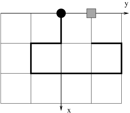
Figure 1: A SAW grafted at the origin $x=y=0$ to a wall placed on the $y$ axis. If the vertex on the wall at $(0,1)$ is not excluded, the only possibility for the next step would be towards this vertex. If this vertex is excluded, the SAW will end at the final point $(1,1)$.

The canonical partition function of walks with $n$ steps ($Z_{n}$) is equal to the number of SAWs starting at the origin and restricted to the half-plane $x\geq 0$, called $c_{n}^{(1)}$ in b78 . The Helmholtz free energy is given by $F_{n}=-k_{B}T\ln c_{n}^{(1)}$. We can estimate the pressure exerted by the SAW at a point $(0,r)$ on the wall by excluding this vertex from the lattice. The excluded vertex is represented as a hatched square in Fig. 1 at $r=1$. The pressure $P_{n}(r)$ exerted at this point is then related to the change in the free energy when the vertex is excluded, $P_{n}a^{2}=-\Delta F_{n}$. If we call $c_{n}^{(1)}(r)$ the number of $n$ step SAWs with the vertex at $(0,r)$ excluded, the dimensionless reduced pressure may be written as

$$p_{n}(r)=\frac{P_{n}(r)a^{2}}{k_{B}T}=-\ln\frac{c_{n}^{(1)}(r)}{c_{n}^{(1)}}.$$ (1)

Of course we are interested in the thermodynamic limit $p(r)=\lim_{n\to\infty}p_{n}(r)$, so the enumeration data must be extrapolated to the infinite length limit. It is worth noting that the density of monomers at the vertex $(0,r)$ is given by $\rho(r)=1-\lim_{n\to\infty}c_{n}^{(1)}(r)/c_{n}^{(1)}$, so that

$$p(r)=-\ln[1-\rho(r)].$$ (2)

The exact enumerations allow us to obtain precise estimates of the pressure exerted by SAW’s at small distances of the grafting point, and we find, rather surprisingly, that the asymptotic form of this pressure is well reproduced even for these small values of $r$. In section II we give some details of the computational enumeration procedure. In section III the enumeration data are analyzed and estimates for the pressure as a function of the distance to the grafting point are presented. Final discussions and conclusions may be found in section IV.

II Exact enumerations

The algorithm we use to enumerate SAWs on the square lattice builds on the pioneering work of Enting ie80 who enumerated square lattice self-avoiding polygons using the finite lattice method. More specifically our algorithm is based in large part on the one devised by Conway, Enting and Guttmann ceg93 for the enumeration of SAWs. The details of our algorithm can be found in j04 . Below we shall only briefly outline the basics of the algorithm and describe the changes made for the particular problem studied in this work.

The first terms in the series for the SAWs generating function can be calculated using transfer matrix techniques to count the number of SAWs in rectangles $W$ vertices wide and $L$ vertices long. Any SAW spanning such a rectangle has length at least $W+L-2$. By adding the contributions from all rectangles of width $W\leq N+1$ and length $W\leq L\leq N-W+1$ the number of SAW is obtained correctly up to length $N$.

The generating function for rectangles with fixed width $W$ are calculated using transfer matrix (TM) techniques. The most efficient implementation of the TM algorithm generally involves bisecting the finite lattice with a boundary (this is just a line in the case of rectangles) and moving the boundary in such a way as to build up the lattice vertex by vertex as illustrated in Fig. 2. If we draw a SAW and then cut it by a line we observe that the partial SAW to the left of this line consists of a number of loops connecting two edges (we shall refer to these as loop ends) in the intersection, and pieces which are connected to only one edge (we call these free ends). The other end of the free piece is either the start-point or the end-point of the SAW so there are at most two free ends.

Each end of a loop is assigned one of two labels depending on whether it is the lower end or the upper end of a loop. Each configuration along the boundary line can thus be represented by a set of edge states $\{\sigma_{i}\}$, where

$$\sigma_{i}=\left\{\begin{array}[]{rl}0&\;\;\;\mbox{empty edge},\\ 1&\;\;\;\mbox{lower loop-end},\\ 2&\;\;\;\mbox{upper loop-end}.\\ 3&\;\;\;\mbox{free end}.\\ \end{array}\right.$$ (3)

If we read from the bottom to the top, the configuration or signature $S$ along the intersection of the partial SAW in Fig. 2 is $S=\{031212120\}$. Since crossings aren’t permitted this encoding uniquely describes which loop ends are connected.

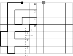
Figure 2: A snapshot of the boundary line (dashed line) during the transfer matrix (TM) calculation on a strip of width 7 with $r=3$. The filled circle indicates the grafted start-point of the SAW and the shaded box the excluded vertex. SAWs are enumerated by successive moves of the kink in the boundary line, as exemplified by the position given by the dotted line, so that one vertex and two edges at a time are added to the strip. To the left of the boundary line we have drawn an example of a partially completed SAW.

The sum over all contributing graphs is calculated as the boundary is moved through the lattice. For each configuration of occupied or empty edges along the intersection we maintain a generating function $G_{S}$ for partial walks with signature $S$. In exact enumeration studies such as this $G_{S}$ is a truncated polynomial $G_{S}(x)$ where $x$ is conjugate to the number of steps. In a TM update each source signature $S$ (before the boundary is moved) gives rise to a few new target signatures $S^{\prime}$ (after the move of the boundary line) and $m=0,1$ or 2 new edges are inserted leading to the update $G_{S^{\prime}}(x)=G_{S^{\prime}}(x)+x^{m}G_{S}(x)$. Once a signature $S$ has been processed it can be discarded. The calculations were done using integer arithmetic modulo several prime numbers with the full integer coefficients reconstructed at the end using the Chinese remainder theorem.

Some changes to the algorithm described in j04 are required in order to enumerate the restricted SAW we study here. Grafting the SAW to the wall can be achieved by forcing the SAW to have a free end (the start-point) on the top side of the rectangle. In enumerations of unrestricted SAW one can use symmetry to restrict the TM calculations to rectangles with $W\leq N/2+1$ and $L\geq W$ by counting contributions for rectangles with $L>W$ twice. The grafting of the start-point to the wall breaks the symmetry and we have to consider all rectangles with $W\leq N+1$. Clearly the number of configurations one must consider grows with $W$. Hence one wants to minimize the length of the boundary line. To achieve this the TM calculation on the set of rectangles is broken into two sub-sets with $L\geq W$ and $L<W$, respectively. The calculations for the sub-set with $L\geq W$ is done as outlined above. In the calculations for the sub-set with $L<W$ the boundary line is chosen to be horizontal (rather than vertical) so it cuts across at most $L+1$ edges. Alternatively, one may view the calculation for the second sub-set as a TM algorithm for SAW with its start-point on the left-most border of the rectangle.

Exclusion of the vertex at distance $r$ from the starting point of the SAW is achieved by blocking this vertex so the walk can’t visit the vertex. The actual calculation can be done in at least two ways. One can simply specify the position of the starting point (and $r$) on the upper/left border and sum over all possible positions. This means doing calculations for a given width $W$ many times; once for each position of the starting point of the SAW. Alternatively one can introduce ‘memory’ into the TM algorithm. Specifically once we have created a configuration which inserts the first free end we ‘remember’ that it did so. We can flag that the free end has been inserted by adding a ghost edge to the configuration initially in state 0. Once the first free end is inserted the state of the ghost edge is changed to $1$. In the next sweep the state of the ghost edge is incremented by 1. When the state of the ghost edge has reached the value $r$ the vertex on the top border is blocked. The problem with the first approach is that we need to do many calculations for any given rectangle. The problem with the second approach is that we need to keep $r+1$ copies of most TM configurations thus using substantially more memory. The choice will be a matter of whether the major computational bottle-neck is CPU time or memory. For this study we used the first approach.

In more detail the TM algorithm for the case $L\geq W$ works as follows. A SAW has two free ends and in the TM algorithm the first free end is forced to be at the top at a distance $k$ from from the left border (this is the starting point of the SAW). We then add a further $r-1$ columns; in the next column the top vertex is forced to be empty. After this further columns are added up to a maximum length of $L_{m}=N-W+1$. This calculation is then repeated for $k=0$ to $L_{m}$ thus enumerating all possible SAWs spanning rectangles of width exactly $W$ and length $L\geq W$. A similar calculation is then done with the SAW grafted to the left border and in each case repeated for all $W\leq N/2$.

The calculation above enumerates almost all possible SAWs. However, we have missed those SAWs with two free ends in the top border where the end-point precedes the starting-point. That is there is a free end in the top border at a distance $>r$ prior to the excluded vertex. We need to count such SAWs separately. The required changes to the algorithm are quite straight-forward and will not be detailed here.

We calculated the number of SAWs up to length $n=59$ for the unrestricted case and for an excluded vertex with $r=1,\,2,\,3,\,4,\,5,\,10$, 20. In each case the calculation was performed in parallel using up to 8 processors, a maximum of some 16GB of memory and using a total of under 2000 CPU hours (see j04 for details of the parallel algorithm). We needed 3 primes to represent each series correctly and the calculations for all the primes were done in a single run.

III Analysis and results

In tables 1 and 2, we have listed the results for the enumerations of self-avoiding walks without additional restrictions, $c_{n}^{(1)}$, and walks which are not allowed to occupy the vertex $(0,1)$ of the wall, $c_{n}^{(1)}(1)$. If we calculate the pressures directly, we notice a parity effect, as seen in the results presented in Fig. 3. This effect is related to an unphysical singularity in the generating function of the counts $c_{n}^{(1)}$, $G(x)=\sum_{n=0}^{\infty}c_{n}^{(1)}x^{n}$. Besides the physical singularity at $x=x_{c}=1/\mu$, where $\mu$ is the connective constant, there is another singularity at $x=-1/\mu$ b78 . This point will be discussed in more detail below, and more precise estimates for the pressures at several distances from the grafting point will be provided.

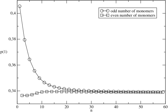
Figure 3: Pressure $p_{n}(r)$ for $r=1$, calculated with the enumeration data for $c_{n}^{(1)}$ and $c_{n}^{(1)}(1)$ using expression (1).

Table 1: Number of walks in the half-plane $c_{n}^{(1)}$.

$n$	$c_{n}^{(1)}$	$n$	$c_{n}^{(1)}$	$n$	$c_{n}^{(1)}$
1	3	21	681552747	41	176707555110156095
2	7	22	1793492411	42	465629874801142259
3	19	23	4725856129	43	1227318029107006037
4	49	24	12439233695	44	3234212894649555857
5	131	25	32778031159	45	8525055738741918835
6	339	26	86295460555	46	22466322857670716727
7	899	27	227399388019	47	59220537922987286933
8	2345	28	598784536563	48	156073168859898607113
9	6199	29	1577923781445	49	411414632591966686887
10	16225	30	4155578176581	50	1084313600069268939547
11	42811	31	10951205039221	51	2858360190045390998925
12	112285	32	28844438356929	52	7533725151809823220637
13	296051	33	76016486583763	53	19860118923927104821817
14	777411	34	200242023748929	54	52346889766180530489735
15	2049025	35	527735162655901	55	137997896899080793506959
16	5384855	36	1390287671021273	56	363744527134008049572583
17	14190509	37	3664208598233159	57	958930393586321187515995
18	37313977	38	9653950752700371	58	2527696511232818406275131
19	98324565	39	25444550692827111	59	6663833305674862002802763
20	258654441	40	67042749110884297

Table 2: Number of restricted walks in the half-plane $c_{n}^{(1)}(1)$.

$n$	$c_{n}^{(1)}(1)$	$n$	$c_{n}^{(1)}(1)$	$n$	$c_{n}^{(1)}(1)$
1	2	21	484553893	41	125845983216200025
2	5	22	1277403184	42	331741159147128245
3	13	23	3361118347	43	874112388226242422
4	35	24	8860136085	44	2304278197456842952
5	91	25	23319106552	45	6071977423574762560
6	242	26	61468398004	46	16006835327039914244
7	630	27	161814936995	47	42181825940070651834
8	1672	28	426530787110	48	111200914189945767681
9	4369	29	1123043680259	49	293056004233059019257
10	11558	30	2960232320818	50	772575890795109134325
11	30275	31	7795418415398	51	2036121996024316003415
12	79967	32	20548006324647	52	5367866589569286706072
13	209779	33	54117914172220	53	14147607361624429924807
14	553634	34	142651034798697	54	37298221266819312654286
15	1453801	35	375747632401071	55	98307470253293931954939
16	3834878	36	990456507011029	56	259178303320281122974230
17	10077384	37	2609158017850105	57	683144867659867533730505
18	26574366	38	6877742334133961	58	1801074652042354959971779
19	69870615	39	18119629209950641	59	4747450605648675761162683
20	184216886	40	47764129557587369

III.1 Critical points and exponents

The critical behaviour of a polymer grafted to a surface is well established dbl93 . It has been proved that the connective constant of grafted walks equals that of unrestricted walks w75 . The associated generating function has a dominant singularity at $x=x_{c}=1/\mu$

$$G(x)=\sum_{n}c_{n}^{(1)}x^{n}\sim A(1-\mu x)^{-\gamma_{1}},$$ (4)

where $\gamma_{1}=61/64$ is a known ds86 ; d89 critical exponent. Besides the physical singularity there is another singularity at $x=x_{-}=-x_{c}$ gw78 ; b78 .

We have analysed the series using differential approximants g89 . We calculate many individual approximants and obtain estimates for the critical points and exponents by an averaging procedure described in chapter 8 of reference g09 . Here and elsewhere uncertainties on estimates from differential apprimants was obtained from the spread among the various approximants as detailed in g09 . The results for unrestricted grafted SAWs are listed in Table 3 under $r=0$. We also list estimates for the cases $r=1,\,2,\,5$ and 10.. From these estimates it is clear that all the series have the same critical behaviour. That is a dominant singularity at $x=x_{c}$ with exponent $-\gamma_{1}=-61/64$ and a non-physical singularity at $x=x_{-}=-x_{c}$ with a critical exponent consistent with the exact value $\gamma_{-}=3/2$.

The critical behavior can be established more rigorously from a simple combinatorial argument. The number of walks $c_{n}^{(1)}(r)$ with the point at $(0,r)$ excluded is clearly less than the number of unrestricted walks $c_{n}^{(1)}$. On the other hand if we attach a single vertical step to the grafting point of an unrestricted walk we get a walk which does not touch the surface at all and hence these walks are a subset of $c_{n}^{(1)}(r)$. This establishes the inequality

$$c_{n-1}^{(1)}\leq c_{n}^{(1)}(r)\leq c_{n}^{(1)},$$ (5)

and hence shows that up to amplitudes the asymptotic behaviors of these sequences are identical.

Table 3: Estimates of the critical points and exponents for SAWs with an excluded vertex a distance $r$ from the origin ($r=0$ is the unrestricted case). The estimates were obtained from third order approximants with $L$ being the degree of the inhomogenous polynomial.

$r$	$L$	$x_{c}$	$\gamma$	$x_{-}$	$\gamma_{-}$
0	0	0.379052260(64)	0.953097(70)	-0.3790526(38)	1.5002(19)
0	4	0.379052241(20)	0.953072(17)	-0.3790492(30)	1.5023(13)
0	8	0.379052243(14)	0.953071(15)	-0.3790498(21)	1.5016(12)
1	0	0.3790522582(30)	0.9530884(24)	-0.3790425(97)	1.5074(74)
1	4	0.3790522575(38)	0.9530879(30)	-0.379030(26)	1.523(29)
1	8	0.379052257(11)	0.953090(14)	-0.379058(16)	1.4988(69)
2	0	0.379052292(16)	0.953123(13)	-0.3790511(33)	1.5011(24)
2	4	0.379052276(12)	0.9531115(97)	-0.3790478(89)	1.5036(60)
2	8	0.379052306(26)	0.953135(20)	-0.379057(21)	1.498(20)
5	0	0.37905218(21)	0.95304(17)	-0.379114(61)	1.457(37)
5	4	0.37905225(31)	0.95313(24)	-0.379099(40)	1.467(29)
5	8	0.37905226(29)	0.95313(25)	-0.379074(31)	1.482(20)
10	0	0.3790483(12)	0.9494(12)	-0.379230(55)	1.369(32)
10	4	0.3790493(40)	0.9503(32)	-0.379237(29)	1.369(14)
10	8	0.3790508(22)	0.9514(14)	-0.379246(91)	1.365(54)

III.2 Pressure

Having established the critical behaviour of the series we can now turn to the determination of the pressure exerted by the polymer on the surface. Since all the series have the same dominant critical behaviour it follows from (1) that the pressure is given by the ratio of the critical amplitudes.

One way of estimating the amplitudes is by a direct fit to an assumed asymptotic form. Here we assume that the asymptotic behaviour of our series is similar to that of unrestricted SAW Caracciolo . The asymptotic analysis of Caracciolo was very thorough and clearly established that the leading non-analytic correction-to-scaling exponent has the value 3/2 (there are also analytic, i.e., integer valued corrections to scaling). We repeated some of the steps in this analysis with the same result for the leading non-analytic correction-to-scaling exponent. Naturally there may be further non-analytic correction-to-scaling exponents with values $>3/2$, but these would be impossible to detect numerically with any degree of certainty. So here we assume that the physical singularity has a leading correction-to-scaling exponent of 1 followed by further half-integer corrections while we assume only integer corrections at the non-physical singularity. We thus fit the coefficients to the asymptotic form

$$c_{n}^{(1)}(r)=\mu^{n}\left[n^{\gamma_{1}-1}\left(A(r)+\sum_{j=2}a_{j}(r)/n^{j/2}\right)+(-1)^{n}n^{-\gamma_{-}-1}\sum_{k=0}b_{k}(r)/n^{k}\right].$$ (6)

In the fits we use the extremely accurate estimate $\mu=2.63815853035(2)$ obtained from an analysis of the series for self-avoiding polygons on the square lattice cj11 and the conjectured exact values $\gamma_{1}=61/64$ and $\gamma_{-}=3/2$. That is we take a sub-sequence of terms $\{c_{n}^{(1)}(r),c_{n-1}^{(1)}(r),\ldots,c_{n-2m-1}^{(1)}(r)\}$, plug into the formula above taking $m$ terms from both the $a_{j}$ and $b_{k}$ sums, and solve the $2m$ linear equations to obtain estimates for the amplitudes.

Figure 4: Estimates for the leading amplitudes obtained by fitting to the asymptotic form (6) plotted against $1/n$ while truncating the asymptotic expansion after 4 to 7 terms.

It is then advantageous to plot estimates for the leading amplitude $A(r)$ against $1/n$ for several values of $m$ as done in Fig. 4. The behaviour of the estimates for the leading amplitudes shown in this figure supports that (6) is a very good approximation to the true asymptotic form. In particular note that the slope becomes very flat as $n$ is increased and decreases as the number of terms $m$ included in the fit is increased. From these plots we estimate $A=1.124705(5)$, $A(1)=0.801625(5)$, $A(2)=0.97564(2)$ and $A(5)=1.09325(10)$, where the uncertainty is a conservative value chosen to include most of the extrapolations from Fig. 4.

The amplitude ratios $A(r)/A$, and hence the pressure, can also be estimated by direct extrapolation of the relevant quotient sequence, using a method due to Owczarek et al. o94 : Given a sequence $\{a_{n}\}$ defined for $n\geq 1$, assumed to converge to a limit $a_{\infty}$ with corrections of the form $a_{n}\sim a_{\infty}(1+b/n+\ldots)$, we first construct a new sequence $\{p_{n}\}$ defined by $p_{n}=\prod_{m=1}^{n}a_{m}$. We then analyse the corresponding generating function

$$P(x)=\sum p_{n}x^{n}\sim(1-a_{\infty}x)^{-(1+b)}.$$

Estimates for $a_{\infty}$ and the parameter $b$ can then be obtained from differential approximants, that is $a_{\infty}$ is just the reciprocal of the first singularity on the positive real axis of $P(x)$. In our case we study the sequence of ratios $a_{n}(r)=c_{n}^{(1)}(r)/c_{n}^{(1)}$, which has the required asymptotic form. Using the same type of differential approximant method outlined above we find that $A/A(1)=1.4030218(5)$, which is entirely consistent with the estimate $A/A(1)=1.403030(15)$ obtained using the amplitude estimates from the direct fitting procedure.

Next we compare these results for the pressure with the ones for gaussian chains as expressed in equation (4) in bick00 . That expression is for polymers in a three-dimensional half-space confined by a two-dimensional wall, and corresponds to finite values of the radius of gyration. If the expression is generalized to the $d$-dimensional case and restricted to the limit of infinite chains, where the radius of gyration diverges, the result is:

$$p_{G}(r)=\frac{P_{G}(r)a^{d}}{k_{B}T}=\frac{\Gamma(d/2)}{\pi^{d/2}}\frac{1}{(r^{2}+1)^{d/2}},$$ (7)

where we recall that $r$ is dimensionless, measured in units of the lattice constant $a$. In table 4 we have listed the estimated pressures for SAWs and the pressures obtained for Gaussian chains in $d=2$, on the semi-infinite square lattice. In Fig. 5 we have plotted the pressure for polymers modelled as SAWs and as Gaussian chains. In this figure the dashed line represents a decay in pressure with the same asymptotic form, $\propto 1/(r^{2}+1)$, as the Gaussian chain but normalised so the curve passes through the SAWs data point for $r=10$. Quite clearly the SAWs data is well represented by this form even for small distances $r>2$. For $r=20$ the SAWs data was indistinguishable from zero pressure.

$r$	$p(r)-SAWs$	$p(r)$-gaussian
1	0.33863	0.15915
2	0.14218	0.06366
3	0.07334	0.03183
4	0.04347	0.01872
5	0.02844	0.01224
10	0.00735	0.00315

Table 4: Pressure at a distance $r$ from the grafting point for SAWs and Gaussian chains.

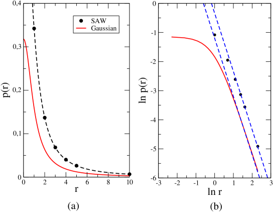
Figure 5: (a) The pressure $p(r)$ exerted by a polymer on a surface at a distance $r$ from the grafting point. Data are for polymers modelled as SAWs or Gaussian chains. The dashed line are a $1/r^{2}$ fit. (b) Both data have the same $1/r^{2}$ scaling form, even for values close to $r=2$. The dashed lines are guide lines with slope equal to $-2$.

IV Final discussions and conclusion

Since our model is athermal and discrete, it is not really possible to compare our results with those obtained for the gaussian chain. However, as was already mentioned by Bickel et al. bick01 , the excluded volume interactions should not change the scaling form of the pressure. Fig. 5(b) clearly shows a $1/r^{2}$ decay of the pressure, even for small distances. According to Bickel et al. bick01 , this similarity is due to the fact that the pressure and the monomer concentration in the vicinity of the wall are linearly related. On the other hand, it seems that the concentration is not affected by the molecular details or by the differences between chain models. In our case, despite the fact that $\rho(r)$ and $p(r)$ are related by a logarithmic relation, as shown in expression (2), we have for $r\gg 1$ a small concentration leading to a linear relation between those quantities. Actually, even for $r\sim 2$, we can observe a linear dependence, as shown in Fig. 6.

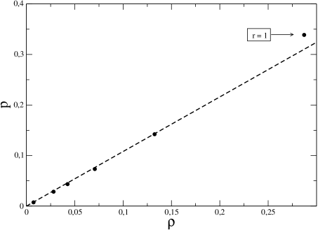
Figure 6: Relation between pressure and concentration of monomers near to the wall at a distance $r$ from the grafting point. For $r>1$, a linear relationship is observed.

Since the grafted chain is in mechanical equilibrium, the force ${\cal F}$ applied to the walk at the grafting point, which is in the negative $x$ direction in Fig. 1, should be equal to the sum of the forces applied by the wall at other contact points, which are in the positive $x$ direction. Thus, the dimensionless force is given by:

$$f=\frac{{\cal F}a}{k_{B}T}=2\sum_{r=1}^{\infty}p(r).$$ (8)

For gaussian chains, integrating equation (7), we find $f_{G}=1$. For SAWs, we may estimate the force summing the results for $r=1,2,\ldots,5$ and obtaining the remaining contributions ($r=6,7,\ldots,\infty$) using the asymptotic result $p(r)\approx A_{p}/(r^{2}+1)$ where $A_{p}\approx 0.74235$ was estimated using the result of $p(r)$ for $r=10$. The result of this calculation is $f_{SAW}\approx 1.533$, larger than the one for gaussian chains. As mentioned above, it does not seem straightforward to compare the two models, since a gaussian chain is a mass-spring model and therefore it is, unlike SAWs, not athermal. We may also mention that if $p(r)$ for SAWs is extended to real values of $r$ using a numerical interpolation procedure and the data for gaussian chains are rescaled so the areas below both curves are the same, the difference between the curves is quite small, the maximum being close to the origin and of order $10^{-3}$. Due to the limited precision of the estimates for SAWs and to the expected small dependency of the results on the interpolation procedure we will not present these results here, but we found that in general the rescaled results for the pressure of gaussian chains are larger than the pressures for SAWs at small values of $r$, but the inverse situation is found for larger distances. This net effect may be understood if we recall that the pressure is a monotonically growing function of the local density at the wall (Eq. (2)) and that the effect of the excluded volume interactions should be a slower decay of this density with the distance from the grafting point, as compared to approximations where this interaction is neglected.

It is of some interest to obtain the total force applied to the chain at the grafting point for ideal chains, modeled by random walks on the semi-infinite square lattice. This force may be calculated considering the shift of the grafting point by one lattice unit in the positive $x$ direction in Fig. 1. The change in free energy under this operation will be proportional to the force. This calculations should lead to the same result of the ones above, where the force was obtained summing over the pressures at all other sites of the wall besides the origin, since the total force applied on the chain has to vanish.

Let us start by briefly reviewing the calculation of the number of random walks on a half-plane of the square lattice. If we call $c_{n}(\vec{\rho})$ the number of $n$-steps random walks on a square lattice starting at the origin and ending at the point $\vec{\rho}=x{\bf i}+y{\bf j}$, the number of RWs on the half-plane $x\geq 0$ may be calculated by placing an absorbing wall at $x=-1$, so that any walk reaching the wall is annihilated. This may be accomplished by using an image walker, starting at the reflection point of the origin with respect to the wall and ending at $\vec{\rho}$. We will place the starting point of the random walk at $(s,0)$, where $s=0$ corresponds to walks starting at the origin. In this case the image walker starting point will be at $\vec{\rho}_{0}=-(s+2){\bf i}$, with distances measured in units of the lattice constant $a$. The number of walks confined to the $x\geq 0$ half plane is given by rg04

$$c^{(1)}_{n}(\vec{\rho},s)=c_{n}(\vec{\rho})-c_{n}(\vec{\rho}+(2+s){\bf i}).$$ (9)

Since we are interested in the large $n$ limit, we may use the gaussian approximation for the number of walks

$$c_{n}(\vec{\rho})=\frac{4^{n}}{n\pi}\exp\left(-\frac{|\vec{\rho}|^{2}}{n}\right).$$ (10)

For the half-plane we get

$$c_{n}^{(1)}(\vec{\rho},s)=\frac{4^{n}}{n\pi}\left[\exp\left(-\frac{|\vec{\rho}|^{2}}{n}\right)-\exp\left(-\frac{|\vec{\rho}+(2+s){\bf i}|^{2}}{n}\right)\right]$$ (11)

To obtain the total number of walks, we integrate this expression over the final point $\vec{\rho}$

$$c_{n}^{(1)}(s)=\int_{0}^{\infty}dx\int_{-\infty}^{\infty}dy\;c_{n}^{(1)}(\vec{\rho},s).$$ (12)

The result is

$$c_{n}^{(1)}(s)=\frac{4^{n}}{\sqrt{\pi}}\int_{-s/\sqrt{n}}^{(2+s)/\sqrt{n}}e^{-x^{2}}dx,$$ (13)

for $n\gg s$, we have the asymptotic behavior

$$c_{n}^{(1)}(s)=4^{n}\frac{2(s+1)}{\sqrt{n\pi}},$$ (14)

which has the expected scaling form (4), with exponent $\gamma=1/2$ and amplitude $A=2(s+1)/\sqrt{\pi}$. The change in free energy between the cases with $s=0$ and $s=1$ is therefore given by $-k_{B}T\ln 2$, so that the force applied to the polymer by the wall at the grafting point will be $f_{RW}=\ln 2\approx 0.6931$, which is lower than the forces obtained for gaussian chains and estimated for SAWs.

It should be mentioned that for SAWs the sum of the pressures corresponding to two distances $p(r_{i})+p(r_{j})$ is always smaller (for finite $|r_{i}-r_{j}|$) than $-\Delta F(r_{i},r_{j})/(k_{B}T)$, where $\Delta F(r_{i},r_{j})$ is the change in free energy when both cells, at $r_{i}$ and $r_{j}$ are excluded. In other words, an effective attractive interaction exists between the two excluded cells, so that the free energy decreases as the cells approach each other. This effect is due to walks in the unrestricted case which visit both excluded cells, and are therefore not counted in either $c_{n}^{(1)}(r_{1})$ or $c_{n}^{(1)}(r_{2})$. The total force $f_{SAW}^{\prime}$, resulting from the simultaneous exclusion of all cells besides the one at the grafting point r = 0, must thus be smaller than the force $f_{SAW}$ defined in equation (8). It is easy to find, since the number of SAWs with $n$ steps $d_{n}^{(1)}$ in this case is given by $d_{n}^{(1)}=1+c_{n-1}^{(1)}$, that for a given value of $n$ the force at the grafting point will be $f^{\prime}_{n,SAW}=-\ln(d_{n}^{(1)}/c_{n}^{(1)})$. For large $n$, we get $f^{\prime}_{SAW}=\ln\mu\approx 0.9701$, smaller than $f_{SAW}=1.533$, as expected.

Finally, we should also stress that although the pressure applied by the SAWs and by the gaussian chains display a similar power-law behavior, other possible walks on the lattice might lead to different results. Recently the pressure exerted by directed walks starting at the origin on the limiting line of a semi-infinite square lattice was obtained rp12 . In the limit of large directed walks the asymptotic decay of the pressure with the distance to the grafting point also follows a power law, albeit with an exponent smaller than the one obtained here for SAWs and gaussian chains.

- (1) B. W. Ninham and P. Lo Nostro, Molecular Forces and Self Assembly: in Colloid, Nano Sciences and Biology, Cambridge University Press (2010).
- (2) S. B. Smith. Y. J. Cui and C. Bustamante, Science 271, 795 (1996).
- (3) P. M. Chaikin and T. C. Lubansky, Principles of Condensed Matter, Cambridge University Press (2000).
- (4) S. Safran, Statistical Thermodynamics of Surfaces, Interfaces and Membranes, Westview Press (1994).
- (5) R. C. Tolman, The Principles of Statistical Mechanics, Dover Publications (1979).
- (6) T. Bickel, C. Marques and C. Jeppesen, Phys. Rev. E 62, 1124 (2000).
- (7) T. Bickel, C. Jeppesen and C. M. Marques, Eur. Phys. J. E 4, 33 (2001).
- (8) M. Breidenich et al, Eur. Phys. Lett. 49, 431 (2000).
- (9) M. N. Barber, A. J. Guttmann, K. M. Middlemiss, G. M. Torrie and S. G. Whittington, J. Phys. A 11, 1833 (1978).
- (10) I. G. Enting, J. Phys. A 13, 3713 (1980).
- (11) A. R. Conway, I. G. Enting and A. J. Guttmann, J. Phys. A 26, 1519 (1993).
- (12) I. Jensen, J. Phys. A 37, 5503 (2004).
- (13) K. De’Bell and T. Lookman, Rev. Mod. Phys. 65, 87 (1993).
- (14) S. G. Whittington, J. Chem. Phys. 63, 779 (1975).
- (15) B. Duplantier and H. Saleur, Phys. Rev. Lett. 57, 3179 (1986).
- (16) B. Duplantier, J. Stat. Phys. 54, 581 (1989).
- (17) A.J. Guttmann and S. G. Whittington, J. Phys. A 11, 721 (1978).
- (18) A. J. Guttmann in Phase Transitions and Critical Phenomena, vol. 13, Academic Press (1989).
- (19) A. J. Guttmann ed., Polygons, Polyominoes and Polycubes vol. 775 of Lecture Notes in Physics, Springer (2009).
- (20) S. Caracciolo, A. J. Guttmann, I. Jensen, A. Pelissetto, A. N. Rogers, and A. D. Sokal, J. Stat. Phys. 120, 1037-1100 (2005).
- (21) N. Clisby and I. Jensen, J. Phys. A 45, 055208 (2012).
- (22) A. L. Owczarek, T. Prellberg, D. Bennett-Wood D and A. J. Guttmann, J. Phys. A 27, L919 (1994).
- (23) J. Rudnick and G. Gaspari, Elements of the Random Walk, Cambridge University Press (2004).
- (24) E. J. J. van Rensburg and T. Prellberg, arXiv:1210.2761 (2012).