Ultrarelativistic Transport Coefficients in Two Dimensions

Abstract

We compute the shear and bulk viscosities, as well as the thermal conductivity of an ultrarelativistic fluid obeying the relativistic Boltzmann equation in $2+1$ space-time dimensions. The relativistic Boltzmann equation is taken in the single relaxation time approximation, based on two approaches, the first, due to Marle and using the Eckart decomposition, and the second, proposed by Anderson and Witting and using the Landau-Lifshitz decomposition. In both cases, the local equilibrium is given by a Maxwell-Jüttner distribution. It is shown that, apart from slightly different numerical prefactors, the two models lead to a different dependence of the transport coefficients on the fluid temperature, quadratic and linear, for the case of Marle and Anderson-Witting, respectively. However, by modifying the Marle model according to the prescriptions given in Ref. [1], it is found that the temperature dependence becomes the same as for the Anderson-Witting model.

1 Introduction

The study of the transport properties of 2D relativistic fluids from the standpoint of kinetic theory is an important topic, still awaiting a complete systematization. Kremer and Devecchi [2] calculated the bulk viscosity of a two dimensional relativistic gas using the Anderson-Witting collision operator and the Chapman-Enskog expansion [3, 4, 5], but did not investigate the shear viscosity and thermal conductivity.

In this paper, we compute the transport coefficients, namely the bulk and shear viscosities and the thermal conductivity, by using two single relaxation time models (also called model equations). The first one, proposed by Marle [6], is appropriate for mildly relativistic fluids with moderate values of the Lorentz factor, $\gamma<2$. The second one, by Anderson and Witting [3], on the other hand, can deal with significantly larger Lorentz factors. The Marle model, as it was initially proposed in Ref. [6], is not appropriate to describe a gas of ultrarelativistic particles, due to the fact that it implies an infinite relaxation time in the limit where the mass of the particles becomes zero, thus leading to divergent transport coefficients. However, Takamoto et al. [1] proposed a modified Marle model, whereby the relaxation time of the Boltzmann equation is redefined in such a way as to regulate the aforementioned infinities. In addition, it is known that by promoting the relaxation time to the status of a dynamic field, it is possible to describe complex flows far from equilibrium, such as they occur in turbulence [7]. Therefore, this single relaxation time model will also be included in the present study of the transport coefficients. In general, model equations do not give the same transport coefficients as the ones obtained from the full Boltzmann equation. However, it was proven in the Ref. [8] that the methods of Chapman-Enskog and Grad lead to the same approximations to transport coefficients, when polynomial expansions of the distribution function in the peculiar velocity are performed.

In both cases, we use the moment expansion of the non-equilibrium distribution, similar to the fourteen fields[4, 9, 5] in the three-dimensional case. To the best of our knowledge, this task has never been undertaken before for the case of two spatial dimensions. This is all but an academic exercise, since two-dimensional relativistic flows arise in many areas of modern physics, say, cosmology, e.g. in galaxy formation from fluctuations in the early universe [10], as well as in high-energy nuclear physics, e.g energetic heavy ions collisions [11]. Two-dimensional ultrarelativistic fluids received a further boost of popularity in 2004, with the discovery of the gapless semiconductor graphene [12, 13]. This consists of literally a single carbon monolayer and represents the first instance of a truly two-dimensional material (the “ultimate flatland”[14]), where electrons move like massless chiral particles, whose dynamics is governed by the Dirac equation, with the Fermi velocity playing the role of the speed of light in relativity [15, 16]. However, the calculation of the transport coefficients is more general and can be extended to any statistical system of quasi-particles governed by relativistic Boltzmann-like equations, i.e. it might apply to a whole class of systems where physical signals are forced to move close to the their ultimate limiting speed [17].

The results of this paper are restricted by the range of applicability of the Boltzmann equation to (quasi) two-dimensional systems. It is well known that linearizing hydrodynamics in two dimensions leads to divergent transport coefficients, both in classical and relativistic systems [18, 19]. However, as long as the Boltzmann equation provides a useful semi-phenomenological approximation to transport phenomena, as for example evidenced by the use of the Boltzmann equation in quantum transport [20], results of our computations remain valid.

We wish to emphasize that the main goal of the present paper is to derive the transport coefficients for $2+1$ dimensional relativistic fluids, out of prescribed relaxation times. In the non-relativistic case, this task is pretty straightforward, since in an absolute reference frame, there is no ambiguity as to the definition of the macroscopic observables (kinetic moments) in terms of the Boltzmann distribution. In the relativistic case, on the other hand, this correspondence, i.e. the projection from the kinetic to the hydrodynamic space, is much less direct and requires careful consideration. Besides its theoretical interest, the practical target of this work is to provide operational input for lattice formulations of the Boltzmann equation, which have recently shown major potential for the numerical simulation of a broad class of relativistic flows across scales, from astrophysical flows, all the way down to quark-gluon plasmas [21, 22, 23, 24], including turbulent phenomena in the two-dimensional electronic gas in graphene [25].

2 Non-Equilibrium Distribution

The single relaxation time Boltzmann equation for the Minkowski metric, $\eta^{\alpha\beta}$, can be written as [4]

$$p^{\mu}\partial_{\mu}f=-\frac{mc}{\tau_{M}}(f-f^{\rm eq})\quad,$$ (1)

for the case of the Marle model [6], and as

$$p^{\mu}\partial_{\mu}f=-\frac{p^{\mu}U_{\mu}}{c^{2}\tau}(f-f^{\rm eq})\quad,$$ (2)

for the case of Anderson and Witting model [3]. Here, $m$ is the mass of the particles, $c$ the speed of light, $k_{B}$ the Boltzmann constant, $f$ the probability distribution function (which can denote any scalar field in phase space), $\tau$ the single relaxation time for the Anderson-Witting model, and $\tau_{M}$ the respective one for the case of the Marle model. The 3-momentum is denoted by $p^{\mu}=(p^{0},\vec{p})$, and the macroscopic 3-velocity by $U^{\mu}$. Greek indices run from $0$ to $2$, being $0$ the temporal component, and we have adopted the Einstein notation (repeated indexes are summed). For the purpose of this work, we are using the signature $(+,-,-)$. The equilibrium distribution $f^{\rm eq}$ is given by [4]

$$f^{\rm eq}=A(n,T)\exp(-p_{\mu}U^{\mu}/k_{B}T)\quad,$$ (3)

where $A(n,T)$ is a normalization constant that depends on the temperature and the number of particles density $n$. In this work, we will study the ultrarelativistic regime, which is characterized by $\xi\equiv mc^{2}/k_{B}T\ll 1$. From now on, we will use natural units, $m=c=k_{B}=1$, and the following notation:

$$\Delta^{\alpha\beta} =\eta^{\alpha\beta}-U^{\alpha}U^{\beta}\quad,$$

$$T^{(\alpha\beta)} =\frac{1}{2}(\Delta^{\alpha}_{\gamma}\Delta^{\beta}_{\delta}+\Delta^{\beta}_{\gamma}\Delta^{\alpha}_{\delta})T^{\gamma\delta}\quad,$$

$$T^{<\alpha\beta>} =T^{(\alpha\beta)}-\frac{1}{2}\Delta^{\alpha\beta}\Delta_{\gamma\delta}T^{(\gamma\delta)}\quad,$$

$$\nabla^{\alpha} =\Delta^{\alpha\beta}\partial_{\beta}\quad.$$ (4)

In order to identify the physical meaning of the different terms in the balance and transport equations, it is useful to introduce decompositions of these terms with respect to orthogonal quantities. Note that $\Delta^{\alpha\beta}$ and $U^{\alpha}$ are orthogonal quantities, $\Delta^{\alpha\beta}U_{\beta}=0$, so that any 3-vector can be decomposed into this orthogonal basis. We begin with the Eckart decomposition [26], and later make the due corrections to take into account the one proposed by Landau and Lifshitz [3, 4].

In the Eckart decomposition, the entropy 3-flow, defined by

$$S^{\alpha}=-\int p^{\alpha}f\ln(f)\frac{d^{2}p}{p^{0}}\quad,$$ (5)

can be written as follows:

$$S^{\alpha}=nsU^{\alpha}+\varphi^{\alpha}\quad,$$ (6)

where $s=S^{\alpha}U_{\alpha}/n$ is the entropy per particle and $\varphi^{\alpha}=\Delta_{\beta}^{\alpha}S^{\beta}$ the entropy flux.

In order to obtain the non-equilibrium distribution, we begin by maximizing the entropy per particle, under the following constraints:

$$N^{\alpha}U_{\alpha} =U_{\alpha}\int p^{\alpha}f\frac{d^{2}p}{p^{0}}\quad,$$

$$T^{\alpha\beta}U_{\alpha} =U_{\alpha}\int p^{\alpha}p^{\beta}f\frac{d^{2}p}{p^{0}}\quad,$$

$$T^{<\gamma\beta>\alpha}U_{\alpha} =U_{\alpha}\int p^{\alpha}p^{<\gamma}p^{\beta>}f\frac{d^{2}p}{p^{0}}\quad,$$ (7)

where,

$$p^{<\alpha}p^{\beta>}=p^{(\alpha}p^{\beta)}-\frac{1}{2}\Delta^{\alpha\beta}\Delta_{\gamma\delta}p^{(\gamma}p^{\delta)}\quad,$$ (8)

and

$$p^{(\alpha}p^{\beta)}=\frac{1}{2}(\Delta^{\alpha}_{\gamma}\Delta^{\beta}_{\delta}+\Delta^{\beta}_{\gamma}\Delta^{\alpha}_{\delta})p^{\gamma}p^{\delta}\quad.$$ (9)

In principle, the moments $N^{\alpha}$ and $T^{\alpha\beta}$ would be a more natural choice. However, the resulting procedure to compute the Lagrange multipliers via entropy maximization, while leading to equivalent results [4], proves significantly more complicated. The problem of maximizing the entropy is equivalent to consider the following functional,

$${\cal{F}}=s-\lambda N^{\alpha}U_{\alpha}-\lambda_{\beta}T^{\alpha\beta}U_{\alpha}-\lambda_{<\gamma\beta>}T^{<\gamma\beta>\alpha}U_{\alpha}\quad,$$ (10)

and applying the functional derivative $\delta{\cal{F}}/\delta f=0$. Here, $\lambda$, $\lambda_{\beta}$, and $\lambda_{<\gamma\beta>}$ are Lagrange multiplier that we must determine. In two dimensions, there are nine independent multipliers, since by definition $\eta^{\gamma\beta}\lambda_{<\gamma\beta>}=0$, which represents an extra equation.

Following the procedure, as a result, one can approximate the non-equilibrium distribution function by,

$$f\simeq f^{\rm eq}\left[1-n\left(\lambda+\lambda_{\beta}p^{\beta}+\lambda_{<\gamma\beta>}p^{\gamma}p^{\beta}\right)\right]\quad.$$ (11)

By decomposing the Lagrange multipliers in the orthogonal basis in space-time,

$$\lambda_{\beta}=\lambda^{\prime}U_{\beta}+\lambda^{\prime}_{\gamma}\Delta^{\gamma}_{\beta}\quad,$$ (12)

$$\lambda_{<\gamma\beta>} =\Lambda U_{\beta}U_{\gamma}+\frac{1}{2}\Lambda_{\alpha}(\Delta_{\gamma}^{\alpha}U_{\beta}+\Delta^{\alpha}_{\beta}U_{\gamma})$$ (13)

$$+\Lambda_{\alpha\delta}\left(\Delta_{\gamma}^{\alpha}\Delta_{\beta}^{\delta}-\frac{1}{2}\Delta^{\alpha\delta}\Delta_{\gamma\beta}\right)\quad.$$

and inserting these variables into the equilibrium distribution, Eq. (11), we obtain

$$f =f^{\rm eq}\bigg{[}1-n\lambda-n\left(\lambda^{\prime}U_{\beta}+\lambda^{\prime}_{\gamma}\Delta^{\gamma}_{\beta}\right)p^{\beta}$$ (14)

$$-n\bigg{(}\Lambda U_{\beta}U_{\gamma}+\frac{1}{2}\Lambda_{\alpha}(\Delta_{\gamma}^{\alpha}U_{\beta}+\Delta^{\alpha}_{\beta}U_{\gamma})$$

$$+\Lambda_{\alpha\delta}\left(\Delta_{\gamma}^{\alpha}\Delta_{\beta}^{\delta}-\frac{1}{2}\Delta^{\alpha\delta}\Delta_{\gamma\beta}\right)p^{\gamma}p^{\beta}\bigg{)}\bigg{]}\quad.$$

In the Grad method, we need to determine the value of the Lagrange multipliers in terms of the macroscopic fields, $n$, $U^{\alpha}$, $T$, $\omega$, $P^{<\alpha\beta>}$, and $q^{\alpha}$ (being the particle density, macroscopic 3-velocity, temperature, dynamic pressure, pressure deviator, and heat flux, respectively). The dynamic pressure is defined by $\omega=-\mu\nabla_{\alpha}U^{\alpha}$, and the pressure deviator by $P^{<\alpha\beta>}=2\eta\nabla^{<\alpha}U^{\beta>}$, being $\mu$ and $\eta$ the bulk and shear viscosities respectively. In this procedure, we also need the moments of the equilibrium distribution function, which have been introduced in Appendix A.

Let us impose that the actual distribution function carries the same first moment as the equilibrium distribution, namely:

$$N^{\alpha}=\int fp^{\alpha}\frac{d^{2}p}{p^{0}}=\int f^{\rm eq}p^{\alpha}\frac{d^{2}p}{p^{0}}\quad,$$ (15)

and apply the projectors, $U_{\alpha}$ and $\Delta_{\alpha}^{\beta}$, to obtain respectively the first two equations for the Lagrange multipliers,

$$-n^{2}[\lambda+2T(3T\Lambda+\lambda^{\prime})] =0\quad,$$

$$nT\lambda^{\prime}_{\gamma}\Delta^{\gamma\beta}+3nT^{2}\Lambda_{\gamma}\Delta^{\gamma\beta} =0\quad.$$ (16)

In order to obtain the other equations, we calculate the energy-momentum tensor,

$$T^{\alpha\beta}=\int fp^{\alpha}p^{\beta}\frac{d^{2}p}{p^{0}}\quad,$$ (17)

and introduce the projectors:

$$\left(\Delta_{\alpha}^{\gamma}\Delta^{\delta}_{\beta}-\frac{1}{2}\Delta^{\gamma\delta}\Delta_{\alpha\beta}\right)T^{\alpha\beta} =P^{<\gamma\delta>}\quad,$$

$$\Delta_{\alpha}^{\gamma}U_{\beta}T^{\alpha\beta} =q^{\gamma}\quad,$$

$$\Delta_{\alpha\beta}T^{\alpha\beta} =-2(p+\omega)\quad,$$

$$U_{\alpha}U_{\beta}T^{\alpha\beta} =\epsilon\quad,$$ (18)

where $\epsilon$ and $p$ are the energy density and hydrostatic pressure, respectively.

Thus, by inserting the distribution function in Eq. (17), and taking the projectors defined in Eq. (2), we obtain the following relations,

$$\omega =-n^{2}T(\lambda+3T(4T\Lambda+\lambda^{\prime}))\quad,$$

$$\epsilon =2nT-2n^{2}T(\lambda+3T(4T\Lambda+\lambda^{\prime}))\quad,$$

$$q^{\gamma} =3n^{2}T^{2}\Delta^{\delta\gamma}\lambda^{\prime}_{\delta}+12n^{2}T^{3}\Delta^{\delta\gamma}\Lambda_{\delta}\quad,$$

$$P^{<\gamma\delta>} =-6n^{2}T^{3}\Lambda^{<\gamma\delta>}\quad.$$ (19)

Note that by imposing the state equation for the ultrarelativistic system, $\epsilon=2nT$, implies that that $\omega$ becomes zero. This is equivalent to say that the bulk viscosity vanishes, like in three dimensions. In addition, this gives $\lambda=-T\lambda^{\prime}$, $\Lambda=-\lambda^{\prime}/6T$, where $\lambda^{\prime}$ can take any value. For simplicity, we will set $\lambda^{\prime}=0$. The arbitrariness on this parameter is due to the fact that, in the ultrarelativistic regime (virtually massless excitations), the number of particles density, $n$, and the temperature of the system, are not independent, since $n\sim T^{2}$ (e.g. gas of photons). In other words, the number of particles density is fixed once the energy density $\epsilon$ of the system is chosen, and therefore one Lagrange multiplier falls apart.

In order to obtain the other Lagrange multipliers, we solve the system of algebraic equations, Eqs. (2) and (2), to obtain:

$$\Delta^{\delta\gamma}\Lambda_{\delta} =\frac{1}{3n^{2}T^{3}}q^{\gamma}\quad,$$

$$\Lambda^{<\gamma\delta>} =-\frac{1}{6n^{2}T^{3}}p^{<\gamma\delta>}\quad,$$

$$\Delta^{\delta\gamma}\lambda^{\prime}_{\delta} =-\frac{1}{n^{2}T^{2}}q^{\gamma}\quad.$$ (20)

Replacing these equations into the definition of the non-equilibrium distribution, we obtain:

$$f=f^{\rm eq}\bigg{[}1+\frac{q_{\beta}p^{\beta}}{nT^{2}} -\frac{1}{3nT^{3}}q_{\gamma}U_{\beta}p^{\gamma}p^{\beta}+\frac{p_{<\gamma\beta>}}{6nT^{3}}p^{\gamma}p^{\beta}\bigg{]}.$$ (21)

This is the non-equilibrium distribution function for a two-dimensional ultrarelativistic system, as expressed in terms of the nine moments. The results described here can also be obtained by using the so-called triangle scheme [27], which is equivalent to the Grad method. In order to calculate the explicit values of the heat flux and the pressure deviator, we have to solve the Boltzmann equation. For the purpose of this study, we choose two approaches for the collision operator, the first one proposed by Marle [6], and the second one by Anderson and Witting [3].

3 3th order moments of the Non-eq Distribution

The third order moment of the distribution function can be calculated as follows:

$$T^{\alpha\beta\gamma}=\int fp^{\alpha}p^{\beta}p^{\gamma}\frac{d^{2}p}{p^{0}}\quad.$$ (22)

By replacing Eq. (21) into this equation and rising the indexes for the nine fields, we obtain for the third order moment,

$$T^{\alpha\beta\gamma} =T^{\alpha\beta\gamma}_{E}+\frac{q^{\epsilon}}{nT^{2}}\eta_{\beta\epsilon}T^{\alpha\beta\gamma\delta}_{E}$$ (23)

$$-\frac{q^{\epsilon}U^{\lambda}}{3nT^{3}}\eta_{\delta\epsilon}\eta_{\sigma\lambda}T^{\alpha\beta\gamma\delta\sigma}_{E}+\frac{P^{<\epsilon\lambda>}}{6nT^{3}}\eta_{\delta\epsilon}\eta_{\sigma\lambda}T^{\alpha\beta\gamma\delta\sigma}_{E}\quad.$$

Note that for an accurate calculation of the third order moment of the distribution function, knowledge up to the fifth order moment of the equilibrium distribution (denoted by subindex $E$) is required. The moments of the equilibrium distribution, Eq. (3), are introduced in Appendix A. Thus, replacing the respective moments of the equilibrium distribution, we obtain the third order moment,

$$T^{\alpha\beta\gamma} =15nT^{2}U^{\alpha}U^{\beta}U^{\gamma}$$ (24)

$$-3nT^{2}(\eta^{\alpha\beta}U^{\gamma}+\eta^{\alpha\gamma}U^{\beta}+\eta^{\beta\gamma}U^{\alpha})$$

$$-2T(\eta^{\alpha\beta}q^{\gamma}+\eta^{\alpha\gamma}q^{\beta}+\eta^{\beta\gamma}q^{\alpha})$$

$$+10T(U^{\alpha}U^{\beta}q^{\gamma}+U^{\alpha}U^{\gamma}q^{\beta}+U^{\beta}U^{\gamma}q^{\alpha})$$

$$+5T(p^{<\alpha\beta>}U^{\gamma}+p^{<\alpha\gamma>}U^{\beta}+p^{<\beta\gamma>}U^{\alpha})\quad.$$

With this expression at hand, we are ready to consider the Boltzmann equation. For the case of the Marle model, we have all the needed quantities in place. However, for the Anderson Witting, some corrections are required, which we shall be introduced in Sec. 3.2.

3.1 Marle Model

For the case of the Boltzmann equation for the Marle model, Eq. (1), it is assumed that,

$$\int f\frac{d^{2}p}{p^{0}} =\int f^{\rm eq}\frac{d^{2}p}{p^{0}}=A=A_{E}\quad,$$

$$\int fp^{\alpha}\frac{d^{2}p}{p^{0}} =\int f^{\rm eq}p^{\alpha}\frac{d^{2}p}{p^{0}}=N^{\alpha}=N_{E}^{\alpha}\quad.$$ (25)

These conditions are satisfied in the Eckart decomposition [26], as in the three dimensional case. The first order moment of the distribution, $N^{\alpha}$, is defined by $nU^{\alpha}$, the second moment is defined by

$$T^{\alpha\beta}=P^{<\alpha\beta>}-p\Delta^{\alpha\beta}+(U^{\alpha}q^{\beta}+U^{\beta}q^{\alpha})+\epsilon U^{\alpha}U^{\beta}\quad,$$ (26)

and the third order moment is calculated as described before, via Eq. (24). These are functions of $U^{\alpha}$, so that we do not need any correction to the moment definitions. By integrating the Boltzmann equation, Eq. (1), in the momentum space, and taking into account the relations (3.1), we obtain, $\partial_{\alpha}N^{\alpha}=0$, and by multiplying the equation by $p^{\beta}$ and repeating the same procedure, we further obtain $\partial_{\alpha}T^{\alpha\beta}=0$. These are the conservation equations for $N^{\alpha}$ and $T^{\alpha\beta}$.

However, by multiplying the equations by $p^{\beta}p^{\gamma}$, we obtain a different equation, $\partial_{\alpha}T^{\alpha\beta\gamma}=-(1/\tau_{M})(T^{\beta\gamma}-T^{\beta\gamma}_{E})$, which contains the information about the transport coefficients. By a standard iteration procedure [4], we can convert this equation into

$$T^{\beta\gamma}-T^{\beta\gamma}_{E}=-\tau_{M}\partial_{\alpha}T^{\alpha\beta\gamma}_{E}\quad.$$ (27)

This means that for the Marle model, we just need to know the third order moment of the equilibrium distribution, and the second order moment of both, the non-equilibrium and equilibrium distributions. The corresponding transport coefficients will be calculated in Sec. 4.

3.2 Anderson-Witting Model

For the case of the Anderson-Witting model, we should use the Landau-Lifshitz decomposition [3, 4]. Such decomposition implies that $U^{\alpha}$ must be calculated, by solving the eigenvalue problem, $T^{\alpha\beta}U_{L\alpha}=\epsilon U_{L\alpha}$ (subindex $L$ denotes Landau-Lifshitz). In general, $U^{\alpha}$, calculated with the Eckart decomposition using $N^{\alpha}=nU^{\alpha}$, will differ from the one calculated with the energy flux, $U_{L}^{\alpha}$. As a consequence, we must find the relation between both quantities and the correct expression for the third order kinetic moment.

In the Landau-Lifshitz decomposition, we assume that $N^{\alpha}U_{\alpha}=N^{\alpha}_{E}U_{\alpha}$, $U_{\alpha}T^{\alpha\beta}=U_{\alpha}T^{\alpha\beta}_{E}$. Moreover, the first and second order moments of the distribution are defined by,

$$N^{\alpha} =nU^{\alpha}_{L}+J^{\alpha}\quad,$$

$$T^{\alpha\beta} =P_{L}^{<\alpha\beta>}-p_{L}\Delta_{L}^{\alpha\beta}+\epsilon_{L}U_{L}^{\alpha}U_{L}^{\beta}\quad.$$ (28)

It can be easily shown that the correspondence between $U^{\alpha}$ and $U^{\alpha}_{L}$ for the ultrarelativisitic case is $U^{\alpha}=U^{\alpha}_{L}-q^{\alpha}/3n$, with $J^{\alpha}=-q^{\alpha}/3T$. The conservation equations $\partial_{\alpha}N^{\alpha}=0$ and $\partial_{\alpha}T^{\alpha\beta}=0$ can be obtained by multiplying by $1$ and $p^{\beta}$, and integrating the Boltzmann equation in the momentum space, respectively.

By multiplying by $p^{\beta}p^{\gamma}$ and applying the Maxwell iteration procedure as before, we obtain:

$$(T^{\alpha\beta\gamma}-T^{\alpha\beta\gamma}_{E})U_{L\alpha}=-\tau\partial_{\alpha}T^{\alpha\beta\gamma}_{E}\quad.$$ (29)

Note that in this case, at variance with the Marle case, the third order moment of the non-equilibrium and equilibrium distribution functions is needed. To calculate the correct expression for the third order moment, it is sufficient to replace $U^{\alpha}$ by $U^{\alpha}_{L}-q^{\alpha}/3n$ into Eq. (24), retaining up to linear terms in the nine fields. This delivers:

$$T^{\alpha\beta\gamma} =15nT^{2}U_{L}^{\alpha}U_{L}^{\beta}U_{L}^{\gamma}$$ (30)

$$-3nT^{2}(\eta^{\alpha\beta}U_{L}^{\gamma}+\eta^{\alpha\gamma}U_{L}^{\beta}+\eta^{\beta\gamma}U_{L}^{\alpha})$$

$$-T(\eta^{\alpha\beta}q^{\gamma}+\eta^{\alpha\gamma}q^{\beta}+\eta^{\beta\gamma}q^{\alpha})$$

$$+5T(U_{L}^{\alpha}U_{L}^{\beta}q^{\gamma}+U_{L}^{\alpha}U_{L}^{\gamma}q^{\beta}+U_{L}^{\beta}U_{L}^{\gamma}q^{\alpha})$$

$$+5T(P^{<\alpha\beta>}U_{L}^{\gamma}+P^{<\alpha\gamma>}U_{L}^{\beta}+P^{<\beta\gamma>}U_{L}^{\alpha})\quad.$$

Everything being in place, we next proceed to calculate the transport coefficients for the two-dimensional ultrarelativistic system, using both decompositions.

4 Transport coefficients

Since we found that the bulk viscosity vanishes, we focus on the shear viscosity and the thermal conductivity. First, let us consider the Marle model and use the expressions (2. By applying the projector $\Delta_{\beta}^{\delta}U_{\gamma}$ to Eq. (27), we obtain the heat flux,

$$q^{\delta}=3nT\tau_{M}\left(\nabla^{\delta}T-\frac{1}{3n}\nabla^{\delta}p\right)\quad,$$ (31)

and by applying the projector $\Delta_{\beta}^{(\epsilon}\Delta^{\delta)}_{\gamma}-\frac{1}{2}\Delta^{\epsilon\delta}\Delta_{\beta\gamma}$, we obtain the pressure deviator,

$$P^{<\alpha\beta>}=6nT^{2}\tau_{M}\nabla^{<\alpha}U^{\beta>}\quad.$$ (32)

From this two relations we can conclude that the transport coefficients in the model of Marle are given by,

$$\kappa_{M}=\frac{3c^{2}k_{B}}{\xi}n\tau_{M},\quad\eta_{M}=\frac{3}{\xi}nk_{B}T\tau_{M},\quad\mu_{M}=0\quad,$$ (33)

being the thermal conductivity, the shear viscosity, and the bulk viscosity, respectively. Note that we have restablished the physical units.

For the case of the Anderson-Witting model, we use Eq. (29) and apply the same projectors, finding

$$q^{\delta}=\frac{3}{8}nT\tau\left(\nabla^{\delta}T-\frac{1}{3n}\nabla^{\delta}p\right)\quad,$$ (34)

for the heat flux and

$$P^{<\alpha\beta>}=\frac{6}{5}nT\tau\nabla^{<\alpha}U^{\beta>}\quad.$$ (35)

for the pressure deviator. With these expressions, the transport coefficients take the form:

$$\kappa_{AW}=\frac{3c^{2}k_{B}}{8}n\tau,\quad\eta_{AW}=\frac{3}{5}nk_{B}T\tau,\quad\mu_{AW}=0\quad.$$ (36)

Here, as in the case of the Marle model, we have restored the physical units. Note that the main difference between the transport coefficients, apart from different numerical prefactors, is that the ones calculated with the Anderson and Witting collision operator have a different dependence on the temperature than the ones calculated with the Marle model (since $\xi$ also depends on $T$).

Considering a non-degenerate gas of relativistic particles in the ultrarelativistic regime, the number of particles density is given by $n=k_{B}^{2}T^{2}/2\pi c^{2}\hbar^{2}$. By taking this into account, we see from Fig. 1 that the thermal conductivity $\kappa_{M}$ decreases with $\xi^{3}$, while $\kappa_{AW}$ with $\xi^{2}$. On the other hand, in Fig. 2, we can observe that the shear viscosity, displays the same qualitative behavior, $\eta_{M}$ decreases with $\xi^{4}$ while $\eta_{AW}$ with $\xi^{3}$. In general, given any relativistic system, one can test which single relaxation time approximation, Marle or Anderson-Witting, better reproduces its behavior. We have considered only values $1/\xi>1$, since our calculations are valid only in this regime.

An interesting calculation is to apply the corrections proposed by Takamoto [1] to the Marle model to account properly for the ultrarelativistic regime, $\xi\rightarrow 0$, of a gas of particles. Although this work was developed in $3+1$ dimensional space-time, we will follow a similar procedure for the case of $2+1$ dimensions. To this purpose, we replace the relaxation time $\tau_{M}$ by its average in momentum space, namely:

$$\tau_{M}=\frac{mc}{n}\int\frac{d^{2}p}{p^{0}}f^{eq}\tau_{rel}=\xi\tau_{rel}\quad,$$ (37)

where $\tau_{rel}$ is now the effective relaxation time of the system and $\tau_{M}$ a simple parameter in the relativistic Boltzmann equation. By replacing this relation in the equations for the transport coefficients in the case of the Marle model, we obtain

$$\kappa_{rel}=3c^{2}k_{B}n\tau_{rel},\quad\eta_{rel}=3nk_{B}T\tau_{rel},\quad\mu_{rel}=0\quad.$$ (38)

Note that these transport coefficients carry the same dependence on temperature as in the case of the Anderson-Witting model. The numerical coefficients, though, are not the same.

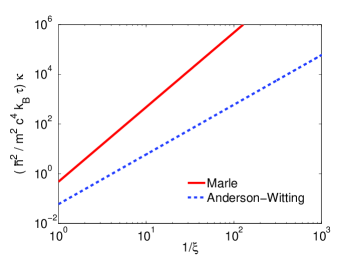
Figure 1: Thermal conductivity $\kappa$ as a function of $\xi$. In this calculation we have set $\tau=\tau_{M}$. The Marle coefficient is systematically higher than the Anderson-Witting one, and the ratio of the two grows at increasing $1/\xi$, i.e. at increasing temperature.

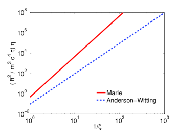
Figure 2: Shear viscosity $\eta$ as a function of $\xi$. In this calculation we have set $\tau=\tau_{M}$. Like for the case of Figure 1, the Marle coefficient is systematically higher than the Anderson-Witting one, and the ratio of the two grows at increasing $1/\xi$, i.e. at increasing temperature.

5 Conclusions and Discussions

In this work, we have calculated the transport coefficients, namely the bulk and shear viscosities, and the thermal conductivity of a two dimensional ultra-relativistic system, using two different forms of the collision operator. The first one is based on the Marle model and the second one on the Anderson Witting approach. Depending on the approach, we have to satisfy the Eckart or the Landau-Lifshitz decompositions, respectively. This leads to different expressions for the transport equations and third order moment of the distribution function.

We have found that the bulk viscosity of the ultrarelativistic system disappears as a consequence of the choice of the two-dimensional ultra-relativistic equation of state, which imposes a constraint on the trace of the momentum-energy tensor. This is the same behavior observed for the three dimensional case. By analyzing the transport coefficients for the case of an ultrarelativistic gas of particles, we have found that the thermal conductivity decreases with $\xi^{3}$ and $\xi^{2}$, for the case of Marle and Anderson-Witting, respectively. The shear viscosity presents the same qualitative behavior, decreasing with $\xi^{4}$ and $\xi^{3}$ for both models, respectively. Therefore, the Marle model transport coefficients always decrease faster than the ones based on the Anderson-Witting model. In a more general relativistic system, by knowing this difference, one could select which one of the two is better suited to describe its dynamics evolution. In addition, following the work by Takamoto [1], we have modified the two-dimensional transport coefficients for the case of the Marle model, in such a way as to make it suitable for a gas of ultra-relativistic particles. With such modification, the functional dependence of the transport coefficients on the temperature becomes the same as for the Anderson-Witting model, although with different numerical coefficients.

It is known that transport coefficients in 2d are formally infrared divergent, hence their size and gradient dependence must be taken with some caution in practical applications [18, 19]. The investigation of these issues in the relativistic framework makes an interesting object of future research.

The results presented in this paper can be applied to a variety of ultrarelativistic systems, e.g. graphene, plasma jets and others. The method is not limited to ultra-relativistic gases of particles, and it extends to any statistical system obeying relativistic Boltzmann-like equations.

Appendix A Moments of the Equilibrium Distribution

The moments of the equilibrium distribution for a two-dimensional ultrarelativistic system that satisfies the Maxwell Jüttner distribution are given by,

$$N_{E}^{\alpha}=nU^{\alpha}\quad,$$ (39)

$$T_{E}^{\alpha\beta}=-nT\eta^{\alpha\beta}+3nTU^{\alpha}U^{\beta}\quad,$$ (40)

$$T_{E}^{\alpha\beta\gamma}=-3nT^{2}(\eta^{\alpha\beta}U^{\gamma} +\eta^{\alpha\gamma}U^{\beta}+\eta^{\beta\gamma}U^{\alpha})$$ (41)

$$+15nT^{2}U^{\alpha}U^{\beta}U^{\gamma}\quad,$$

$$T_{E}^{\alpha\beta\gamma\delta} =3nT^{3}(\eta^{\alpha\beta}\eta^{\gamma\delta}+\eta^{\alpha\gamma}\eta^{\beta\delta}+\eta^{\gamma\beta}\eta^{\alpha\delta})$$ (42)

$$-15nT^{3}(\eta^{\alpha\beta}U^{\gamma}U^{\delta}+\eta^{\alpha\gamma}U^{\beta}U^{\delta}+\eta^{\gamma\beta}U^{\alpha}U^{\delta}$$

$$+\eta^{\alpha\delta}U^{\gamma}U^{\beta}+\eta^{\delta\gamma}U^{\beta}U^{\alpha}+\eta^{\delta\beta}U^{\alpha}U^{\gamma})$$

$$+105nT^{3}U^{\alpha}U^{\beta}U^{\gamma}U^{\delta}\quad,$$

$$T_{E}^{\alpha\beta\gamma\delta\epsilon} =15nT^{4}[U^{\epsilon}(\eta^{\alpha\beta}\eta^{\gamma\delta}+\eta^{\alpha\gamma}\eta^{\beta\delta}+\eta^{\gamma\beta}\eta^{\alpha\delta})$$ (43)

$$+U^{\alpha}(\eta^{\epsilon\beta}\eta^{\gamma\delta}+\eta^{\epsilon\gamma}\eta^{\beta\delta}+\eta^{\gamma\beta}\eta^{\epsilon\delta})$$

$$+U^{\beta}(\eta^{\alpha\epsilon}\eta^{\gamma\delta}+\eta^{\alpha\gamma}\eta^{\epsilon\delta}+\eta^{\gamma\epsilon}\eta^{\alpha\delta})$$

$$+U^{\beta}(\eta^{\alpha\epsilon}\eta^{\gamma\delta}+\eta^{\alpha\gamma}\eta^{\epsilon\delta}+\eta^{\gamma\epsilon}\eta^{\alpha\delta})$$

$$+U^{\gamma}(\eta^{\alpha\beta}\eta^{\epsilon\delta}+\eta^{\alpha\epsilon}\eta^{\beta\delta}+\eta^{\epsilon\beta}\eta^{\alpha\delta})$$

$$+U^{\delta}(\eta^{\alpha\beta}\eta^{\gamma\epsilon}+\eta^{\alpha\gamma}\eta^{\beta\epsilon}+\eta^{\gamma\beta}\eta^{\alpha\epsilon})]$$

$$-105nT^{4}(\eta^{\alpha\beta}U^{\gamma}U^{\delta}U^{\epsilon}+\eta^{\alpha\gamma}U^{\beta}U^{\delta}U^{\epsilon}$$

$$+\eta^{\alpha\delta}U^{\beta}U^{\gamma}U^{\epsilon}+\eta^{\delta\gamma}U^{\alpha}U^{\beta}U^{\epsilon}$$

$$+\eta^{\delta\beta}U^{\alpha}U^{\gamma}U^{\epsilon}+\eta^{\beta\gamma}U^{\alpha}U^{\delta}U^{\epsilon}$$

$$+\eta^{\alpha\epsilon}U^{\beta}U^{\gamma}U^{\delta}+\eta^{\beta\epsilon}U^{\alpha}U^{\gamma}U^{\delta}+\eta^{\gamma\epsilon}U^{\alpha}U^{\beta}U^{\delta})$$

$$+945nT^{4}U^{\alpha}U^{\beta}U^{\gamma}U^{\delta}U^{\epsilon}\quad.$$

To obtain the moments, we have considered the ultrarelativistic regime, $\xi\ll 1$.

References

References

- [1] M. Takamoto and S. Inutsuka. The relativistic kinetic dispersion relation: Comparison of the relativistic Bhatnagar-Gross-Krook model and Grad’s 14-moment expansion. Physica A: Statistical Mechanics and its Applications, 389(21):4580 – 4603, 2010.
- [2] G. M. Kremer and F. P. Devecchi. Thermodynamics and kinetic theory of relativistic gases in 2d cosmological models. Phys. Rev. D, 65:083515, Apr 2002.
- [3] J. L. Anderson and H. R. Witting. A relativistic relaxation-time for the Boltzmann equation. Physica, 74:466, 1974.
- [4] C. Cercignani and G. M. Kremer. The Relativistic Boltzmann Equation: Theory and Applications. Boston; Basel; Berlin: Birkhauser, 2002.
- [5] C. Cercignani and G.M. Kremer. Moment closure of the relativistic Anderson and Witting model equation. Physica A: Statistical Mechanics and its Applications, 290(1–2):192 – 202, 2001.
- [6] C. Marle. Modèle cinétique pour l’ètablissement des lois de la conduction de la chaleur et de la viscositè en thèorie de la relativitè. C. R. Acad. Sc. Paris, 260:6539–6541, 1965.
- [7] H. Chen, S. Kandasamy, S. Orszag, R. Shock, S. Succi, and V. Yakhot. Extended Boltzmann kinetic equation for turbulent flows. Science, 1:633–636, 2003.
- [8] S. Reinecke and G.M. Kremer. A generalization of the Chapman-Enskog and Grad methods. Continuum Mechanics and Thermodynamics, 3:155–167, 1991.
- [9] Henning Struchtrup. Projected moments in relativistic kinetic theory. Physica A: Statistical Mechanics and its Applications, 253(1–4):555 – 593, 1998.
- [10] Bernard J. T. Jones. The origin of galaxies: A review of recent theoretical developments and their confrontation with observation. Rev. Mod. Phys., 48:107–149, Jan 1976.
- [11] A.S. Goldhaber and H.H. Heckman. High energy interactions of nuclei. Ann. Rev. Nucl. Part. Sci., 28:161, 1978.
- [12] K. S. Novoselov, A. K. Geim, S. V. Morozov, D. Jiang, M. I. Katsnelson, I. V. Grigorieva, and S. V. Dubonos. Two-dimensional gas of massless Dirac fermions in graphene. Nature Letters, 438(10):197, Nov 2005.
- [13] K. S. Novoselov, A. K. Geim, S. V. Morozov, D. Jiang, Y. Zhang, S. V. Dubonos, I. V. Grigorieva, and A. A. Firsov. Electric Field Effect in Atomically Thin Carbon Films. Science, 306(5696):666–669, 2004.
- [14] A. K. Geim and A. H. MacDonald. Graphene: Exploring carbon flatland. Phys. Today, page 35, August 2007.
- [15] A. H. Castro Neto, F. Guinea, N. M. R. Peres, K. S. Novoselov, and A. K. Geim. The electronic properties of graphene. Rev. Mod. Phys., 81:109–162, Jan 2009.
- [16] N. M. R. Peres. Colloquium: The transport properties of graphene: An introduction. Rev. Mod. Phys., 82:2673–2700, Sep 2010.
- [17] S. Succi M. Mendoza, N. A. M. Araújo and H. J. Herrmann. Transition in the equilibrium distribution function of relativistic particles. Sci. Rep., 2:611, 2012.
- [18] B. J. Alder and T. E. Wainwright. Velocity autocorrelations for hard spheres. Phys. Rev. Lett., 18:988–990, 1967.
- [19] Henk van Beijeren. Exact results for anomalous transport in one-dimensional Hamiltonian systems. Phys. Rev. Lett., 108:180601, Apr 2012.
- [20] S. Das Sarma, S. Adam, E. H. Hwang, and E. Rossi. Electronic transport in two-dimensional graphene. Rev. Mod. Phys., 83:407–470, May 2011.
- [21] R. Benzi, S. Succi, and Vergassola. The lattice Boltzmann equation: theory and applications. Phys. Rep., 222:145, 1992.
- [22] S. Chen and G. Doolen. Lattice Boltzmann method for fluid flows. Annu. Rev. Fluid Mech., 30:329–364, 1998.
- [23] M. Mendoza, B. M. Boghosian, H. J. Herrmann, and S. Succi. Fast lattice Boltzmann solver for relativistic hydrodynamics. Phys. Rev. Lett., 105:014502, 2010.
- [24] D. Hupp, M. Mendoza, I. Bouras, S. Succi, and H. J. Herrmann. Relativistic lattice Boltzmann method for quark-gluon plasma simulations. Phys. Rev. D, 84:125015, Dec 2011.
- [25] M. Mendoza, H. J. Herrmann, and S. Succi. Preturbulent regimes in graphene flow. Phys. Rev. Lett., 106(15):156601, Apr 2011.
- [26] Carl Eckart. The thermodynamics of irreversible processes. iii. relativistic theory of the simple fluid. Phys. Rev., 58:919–924, Nov 1940.
- [27] A.N. Gorban and I.V. Karlin. Invariant Manifolds for Physical and Chemical Kinetics. Springer, Berlin Heidelberg, 2004.