Recurrent Online Clustering as a Spatio-Temporal Feature Extractor in DeSTIN
Abstract
This paper presents a basic enhancement to the DeSTIN deep learning architecture by replacing the explicitly calculated transition tables that are used to capture temporal features with a simpler, more scalable mechanism. This mechanism uses feedback of state information to cluster over a space comprised of both the spatial input and the current state. The resulting architecture achieves state-of-the-art results on the MNIST classification benchmark.
1 Introduction
We introduce an enhancement to DeSTIN [1] that is aimed at simplifying the architecture and improving its ability to capture temporal features. The DeSTIN architecture consists of multiple instantiations of a common node arranged into layers. Using the recurrent clustering algorithm presented, spatiotemporal dependencies are naturally captured throughout the hierarchy. This recurrent clustering algorithm replaces the earlier incremental clustering algorithm and state-transition table which previously constructed the core of the DeSTIN node. Each node operates independently and in parallel to all others which makes this architecture particularly well-suited to implementation in parallel hardware. The changes made here make the task of a parallel implementation, whether it be on a GPU or in custom analog circuitry, much more achievable.
2 Recurrent Clustering Algorithm
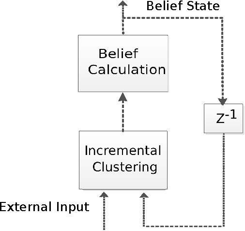
In this section we will describe a recurrent incremental clustering algorithm that forms centroids on a space comprised of a concatenation of the current spatial input and the previous belief state. The belief state represents the probability that the current combination of external observation and internal belief state belongs to each of the centroids.
2.1 Incremental Clustering
The core of this recurrent clustering system is a winner-take-all clustering algorithm that maintains estimates for the mean, , and a variance, , for each dimension of each centroid [2]. These are updated according to eqs. (1) and (2). In these equations is the current observation, is the centroid being updated, and are learning rates. In order to handle cases of poor centroid initialization, a mechanism called starvation trace is employed to help select the centroid to be updated, as outlined in eqs. (3) and (4). The starvation trace, , decays with time when a centroid is not selected for an update. This value is used to weight the distance between the corresponding centroid and the observation, such that centroids which are distant from all observations can be updated.
| (1) |
| (2) |
| (3) |
| (4) |
2.2 Belief State Formulation
Once the selected centroid is updated, the elements of the belief state, , are updated using the normalized Euclidean distance between the -dimensional input vector, , and each centroid, , in the set of centroids, , as shown in eqs. (5) and (6).
| (5) |
| (6) |
2.3 Feedback Construct

This belief state is used as a portion of the input to the core clustering algorithm, as depicted in Figure 1. Introducing this feedback raises the concern of balancing the importance of the spatial input and the temporal belief in the selection algorithm. If the temporal component is not given adequate weight, this feedback loop will have no effect. If, however, it is given too much weight, the spatial element may be ignored. It was sufficient to employ a simple Euclidean distance measure to select the winning centroid. However, if the distributions of the spatial input and the belief states are vastly different, it may be necessary to use a normalized Euclidean distance with a constant normalization vector, the elements of which serve as weights for each dimension.
3 Simulation Results
Here we report on a series of experiments designed to demonstrate the ability of the revised DeSTIN architecture to represent temporal information. First, we explore the recurrent clustering algorithm’s abilities on a simple sequence analysis test case, and then the performance of the algorithm in a full-scale architecture is demonstrated on a couple of standard benchmarks.
3.1 Recurrent Clustering for Sequence Detection

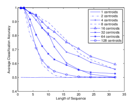
It is important that the recurrent clustering be able to capture regularities across time. In order to demonstrate this capability, binary sequence detection tasks were studied with varying lengths for the sequence of interest. The clustering algorithm is presented with equal probability either the sequence of interest, or a sequence identical to it with only the first element inverted. The belief states for each of the sequences were provided to a feed-forward neural network for the purpose of classifying each sequence. Figure 2 illustrates an exponentially-decaying relationship between the classification accuracy and the length of the sequence of interest. This is to be expected given that there is no supervision to guide the algorithm in capturing temporal dependencies of any specific length. The results highlight that if too few centroids are considered, the algorithm has insufficient resources to represent dependencies that span longer time intervals. If too many centroids are used, the belief state may capture features in the data not relevant to identifying the sequence of interest. However, such sensitivity to the number of centroids is desirably weak.
3.2 MNIST Dataset
The revised clustering scheme was next used in a full-scale architecture and applied to the MNIST dataset classification problem [3]. The DeSTIN hierarchy used was made up of layers of nodes with each layer consisting , and nodes from bottom to top. The bottom layer viewed a window that is shifted over the image, with each bottom layer node receiving a unique patch. The bottom, middle, and top layer nodes used , , and centroids, respectively. The hierarchy was then trained on of the training set images. Next, all training images and testing images were provided to the hierarchy in order to generate feature vectors. The feature vector for each image consisted of each node’s belief state sampled at every movement. These feature vectors were provided to an ensemble of 11 feed-forward neural networks trained with negative correlation learning. Each FFNN consisted of two hidden layers, with 128 and 64 hidden neurons in the first and second layer respectively. A classification accuracy of was achieved which is comparable to results using the first-generation DeSTIN architecture [1] and to results achieved with other state-of-the-art methods [4, 5, 6].
References
- [1] T. P. Karnowski, Deep Machine Learning with Spatio-Temporal Inference. PhD thesis, The University of Tennessee, Knoxville, Tennessee, May 2012.
- [2] S. Young, I. Arel, T. Karnowski, and D. Rose, “A fast and stable incremental clustering algorithm,” in in 7th International Conference on Information Technology, April 2010.
- [3] Y. Lecun and C. Cortes, “The MNIST database of handwritten digits,” March 2009.
- [4] B. Kégl and R. Busa-Fekete, “Boosting products of base classifiers,” in Proceedings of the 26th Annual International Conference on Machine Learning, ICML ’09, (New York, NY, USA), pp. 497–504, ACM, 2009.
- [5] R. Salakhutdinov and G. Hinton, “Learning a nonlinear embedding by preserving class neighbourhood structure,” in Proceedings of the International Conference on Artificial Intelligence and Statistics, vol. 11, 2007.
- [6] P. Simard, D. Steinkraus, and J. Platt, “Best practices for convolutional neural networks applied to visual document analysis,” in Document Analysis and Recognition, 2003. Proceedings. Seventh International Conference on, pp. 958 – 963, Aug. 2003.