Density Perturbations
from Modulated Decay of the Curvaton

David Langlois¹ and Tomo Takahashi²

¹APC (CNRS-Université Paris 7), 10, rue Alice Domon et Léonie Duquet, 75205
Paris Cedex 13, France
²Department of Physics, Saga University, Saga 840-8502, Japan

We study density perturbations, including their non-Gaussianity, in models in which the decay rate of the curvaton depends on another light scalar field, denoted the modulaton. Although this model shares some similarities with the standard curvaton and modulated reheating scenarios, it exhibits interesting predictions for $f_{\rm NL}$ and $g_{\rm NL}$ that are specific to this model. We also discuss the possibility that both modulaton and curvaton fluctuations contribute to the final curvature perturbation. Our results naturally include the standard curvaton and modulated reheating scenarios as specific limits and are thus useful to present a unified treatment of these models and their variants.

1 Introduction

Cosmological observations are increasingly precise, providing us with a lot of information on the origin of cosmic structure, i.e. on primordial density fluctuations. Although the fluctuations of the inflaton field are considered as the main candidate for their origin, other possibilities have also been investigated (see e.g. [1] for introductory lectures), especially in the light of recent constraints on primordial non-Gaussianity. The degree of non-Gaussianity in primordial density fluctuations is usually characterized by the non-linearity parameter $f_{\rm NL}$ which represents the amplitude of the bispectrum. In the case of standard slow-roll single-field inflation, $f_{\rm NL}$ is predicted to be too small to be observable. On the other hand, the present constraints on $f_{\rm NL}$ for local type non-Gaussianity obtained from cosmic microwave background (CMB) and large scale structure are respectively $f_{\rm NL}^{\rm(local)}=37.2\pm 19.9$ (1$\sigma$ C.L.) from WMAP9 [2] and $f_{\rm NL}^{\rm(local)}=62\pm 27$ (1$\sigma$ C.L.) from NRAO VLA Sky Survey [3], which may give some hints that the value of $f_{\rm NL}$ is away from zero.

In this context, other candidates for primordial fluctuations, in particular those giving significant $f_{\rm NL}$, have been extensively discussed such as the curvaton model [4, 5, 6], modulated reheating scenario [7, 8], inhomogeneous end of hybrid inflation [9, 10, 11, 12], modulated trapping [13, 14] and so on. Even if we limit ourselves to the curvaton and modulated reheating scenarios, various extensions of them have been proposed and studied, for example mixed inflaton-curvaton model [15, 16, 17, 18, 19], mixed inflaton-modulated reheating model [20], multi-curvaton [21, 22], modulated curvaton [23, 24] and so on. In most of those scenarios, a light scalar field (degree of freedom) other than the inflaton is involved in some way, and the final values of density perturbations depend on how the initial fluctuations are converted to the final ones during the evolution of the early Universe. This consideration provides a strong motivation to treat models involving curvatons and/or modulatons in a unified formalism (see [34]). In the present work, we wish to focus our attention on a scenario that interpolates between the modulated reheating and the curvaton models: that of the modulated curvaton decay, in which the decay of the curvaton field is modulated by the dependence of its decay rate $\Gamma$ on another fluctuating scalar field, which we will call the modulaton.

In this paper, we focus on this new mechanism of generating primordial density fluctuations and derive its predictions, paying particular attention to non-Gaussianities by computing the bispectrum and trispectrum. Although the model we propose here is, in some sense, a straightforward extension of the curvaton and modulated reheating scenarios, we find that it leads to a rich phenomenology, with interesting observational implications for primordial non-Gaussianity. We also provide general formulas, which could be applied to other similar types of scenarios (see [34] for a systematic approach, including isocurvature perturbations).

The structure of this paper is as follows. In the next section, we derive a general expression describing the final curvature perturbation, up to third order in the perturbations. Focussing then, in Section 3, on the modulaton fluctuations, we analyse the density perturbation and compute the non-linear parameters such as $f_{\rm NL}$ and $g_{\rm NL}$. In Section 4, we investigate models in which the curvaton fluctuations also contribute to the observed perturbations in addition to those from the modulaton. The final section contains a summary of this paper.

2 Computing the post-decay perturbation

The present scenario relies on the presence of three scalar fields: an inflaton field $\phi$ which drives the inflationary expansion; a curvaton (or modulus) field $\sigma$, with an energy density negligible during inflation, which, well after inflation, oscillates at the bottom of its potential before decaying; and, finally, a modulaton field $\chi$, which is light during inflation and thus acquires fluctuations from the amplification of quantum fluctuations. The crucial assumption here is that the decay rate of the curvaton $\sigma$ depends on the modulaton $\chi$. Therefore, fluctuations of $\chi$ directly lead to a varying decay rate and eventually produce density fluctuations.

In practice, we will not need any detail about the inflaton field. Its role will be simply to drive inflation so that the modulaton field can acquire some fluctuations. In our scenario, $\sigma$ can be either light during inflation ($m_{\sigma}\ll H$), in which case it will also acquire some fluctuations, or be massive ($m_{\sigma}\gg H$) in which case its fluctuations are suppressed. Strictly speaking, the curvaton scenario assumes a light field during inflation, but there exist models where the additional scalar fields, such as moduli, are not necessary light during inflation. Whereas the original curvaton scenario would not apply to scalar fields of this type, our model does. In the following, although $\sigma$ is a scalar field, we will be interested in the cosmological phase where it oscillates at the bottom of its potential and can be effectively described as a fluid, which is pressureless if the potential is quadratic. Note that our formalism also applies to the decay of the inflaton oscillating in a quadratic potential at the end of inflation, if $\sigma$ is simply replaced by the inflaton $\phi$. Our formalism thus includes automatically the modulated reheating scenario.

For each fluid characterized by an equation of state parameter $w_{i}\equiv P_{i}/\rho_{i}$, which is assumed here to be constant, it is convenient to introduce the non-linear curvature perturbation $\zeta_{i}$ [35] (see also [36, 37, 38] for a covariant definition)

$$\zeta_{i}=\delta N+\frac{1}{3(1+w_{i})}\ln\left(\frac{\rho_{i}(t,\vec{x})}{\bar{\rho}_{i}(t)}\right),$$ (1)

where $\delta N$ denotes the local perturbation of the number of e-folds and a barred quantity must be understood as homogeneous. From the above formula, the nonlinear energy density of the species $i$ can be written locally as

$$\rho_{i}(t,\vec{x})=\bar{\rho}_{i}(t)e^{3(1+w_{i})(\zeta_{i}-\delta N)}.$$ (2)

In our case, we will consider only two species: radiation ($w_{r}=1/3$) and the curvaton field, treated as a pressureless fluid ($w_{\sigma}=0$).

Using the instantaneous decay approximation, the value of the Hubble parameter at the decay of the curvaton $\sigma$ (or, alternatively, of the inflaton to describe inhomogeneous reheating) is given by

$$H=\Gamma(\chi),$$ (3)

where the decay rate $\Gamma$ is a function of the modulaton $\chi$. Because of the modulaton fluctuations $\delta\chi=H/(2\pi)$ generated during inflation, the decay hypersurface characterized by the above relation is inhomogeneous. Using Friedmann’s equations, this implies for the local energy density

$$\frac{\rho_{\rm tot}(t_{D},\vec{x})}{\bar{\rho}_{\rm tot}(\bar{t}_{D})}=\frac{H^{2}(t_{D},\vec{x})}{\bar{H}^{2}({t}_{D})}=\frac{\Gamma^{2}(t_{D},\vec{x})}{\bar{\Gamma}^{2}(\bar{t}_{D})},$$ (4)

where $t_{D}(\vec{x})$ represents the local decay time. Substituting

$$\rho_{\rm tot}(t_{D},\vec{x})=\sum_{i}\rho_{i}(t_{D},\vec{x})=\sum_{i}\bar{\rho}_{i}(\bar{t}_{D})\,e^{3(1+w_{i})(\zeta_{i}-\delta N_{D})}$$ (5)

in the relation (4), both for the matter contents just before and just after decay, we find

$$(1-\Omega_{\sigma})\,e^{4(\zeta_{r}-\delta N_{D})}+\Omega_{\sigma}\,e^{3(\zeta_{\sigma}-\delta N_{D})}=\left(1+\delta_{\Gamma}\right)^{2}=e^{4(\zeta-\delta N_{D})},$$ (6)

where we have introduced the curvaton fraction of the total energy density (just before the decay) $\Omega_{\sigma}\equiv\bar{\rho}_{\sigma}/\bar{\rho}_{\rm tot}$, as well as the (nonlinear) relative fluctuations of the decay rate

$$\delta_{\Gamma}\equiv\frac{\Gamma(t_{D},\vec{x})}{\bar{\Gamma}(\bar{t}_{D})}-1\,.$$ (7)

The first equality in (6) gives us the expression of $\delta N_{D}$ as a function of the two pre-decay curvature perturbations $\zeta_{r}$ and $\zeta_{\sigma}$. And the second equality in (6) yields the expression of the post-decay curvature perturbation $\zeta$ (carried by the only-remaining radiation fluid) as a function of $\delta N_{D}$, namely

$$\zeta=\delta N_{D}+\frac{1}{2}\ln(1+\delta_{\Gamma})\,.$$ (8)

There is no general nonlinear expression for $\delta N_{D}$ given in terms of $\zeta_{r}$ and $\zeta_{\sigma}$, but by expanding the first equality of (6) order by order in the perturbations, one can iteratively obtain an explicit expression for $\delta N_{D}$ valid up to any order. Computing $\delta N_{D}$ up to third order with this method and substituting in (8), we finally get the following expression for the post-decay curvature perturbation:

$$\zeta = \zeta_{r}-\frac{r}{6}\delta_{\Gamma}+\frac{r}{3}S-\frac{r}{72}\left[\left(r^{2}+2r-9\right)\delta_{\Gamma}^{2}+4\left(r^{2}+2r-3\right)S^{2}-4\left(r^{2}+2r-3\right)S\delta_{\Gamma}\right]$$

$$+\frac{r}{1296}\left[\left(-3r^{4}-10r^{3}+22r^{2}+54r-135\right)\delta_{\Gamma}^{3}+8\left(3r^{4}+10r^{3}-4r^{2}-18r+9\right)S^{3}\right.$$

$$\left.\ -12\left(3r^{4}+10r^{3}-4r^{2}-18r+9\right)S^{2}\delta_{\Gamma}+6\left(3r^{4}+10r^{3}-10r^{2}-30r+27\right)S\delta_{\Gamma}^{2}\right],$$

where we have introduced, for convenience, the curvaton isocurvature perturbation

$$S\equiv 3(\zeta_{\sigma}-\zeta_{r})$$ (10)

and the parameter $r$, defined by

$$r\equiv\left.\frac{3\bar{\rho}_{\sigma}}{4\bar{\rho}_{r}+3\bar{\rho}_{\sigma}}\right|_{D}=\frac{3\,\Omega_{\sigma}}{4-\Omega_{\sigma}}\,.$$ (11)

Although isocurvature fluctuations can also be generated in principle, we restrict our analysis to adiabatic perturbations in the present work (see [34] for an analysis including isocurvature modes).

Note that the perturbations $\zeta_{r}$, $\zeta_{\sigma}$ and $\delta_{\Gamma}$ are related to the fluctuations of the inflaton, curvaton and modulaton, via the expressions

$$\zeta_{r}=\frac{H}{\dot{\phi}}\delta\phi,\quad S=\frac{2\delta\sigma}{\sigma}-\frac{\delta\sigma^{2}}{\sigma^{2}}+\frac{2}{3}\frac{\delta\sigma^{3}}{\sigma^{3}},\quad\delta_{\Gamma}=\frac{\Gamma^{\prime}}{\Gamma}\delta\chi+\frac{\Gamma^{\prime\prime}}{2\Gamma}\delta\chi^{2}+\frac{\Gamma^{{}^{\prime\prime\prime}}}{6\Gamma}\delta\chi^{3},$$ (12)

where a prime denotes the derivatives with respect to $\chi$. Substituting the above expressions in (2) would thus give the curvature perturbation $\zeta$ as a function of the fluctuations $\delta\phi$, $\delta\sigma$ and $\delta\chi$.

Once the curvature perturbation has been computed, here up to third order, it is useful, in order to confront the model with observations, to calculate the power spectrum $P_{\zeta}$, bispectrum $B_{\zeta}$ and trispectrum $T_{\zeta}$. They correspond, respectively, to the 2-point, 3-point and 4-point correlation functions in Fourier space:

$$\langle\zeta_{{\bm{k}}_{1}}\zeta_{{\bm{k}}_{2}}\rangle = (2\pi)^{3}\delta({\bm{k}}_{1}+{\bm{k}}_{2})P_{\zeta}(k_{1})\,,$$ (13)

$$\langle\zeta_{{\bm{k}}_{1}}\zeta_{{\bm{k}}_{2}}\zeta_{{\bm{k}}_{3}}\rangle = (2\pi)^{3}\delta({\bm{k}}_{1}+{\bm{k}}_{2}+{\bm{k}}_{3})B_{\zeta}(k_{1},k_{2},k_{3})\,,$$ (14)

$$\langle\zeta_{{\bm{k}}_{1}}\zeta_{{\bm{k}}_{2}}\zeta_{{\bm{k}}_{3}}\zeta_{{\bm{k}}_{4}}\rangle = (2\pi)^{3}\delta({\bm{k}}_{1}+{\bm{k}}_{2}+{\bm{k}}_{3}+{\bm{k}}_{4})T_{\zeta}(k_{1},k_{2},k_{3},k_{4})\,.$$ (15)

In the case of local non-Gaussianity, it is convenient to express the bispectrum and trispectrum in terms of the power spectrum and to introduce the so-called non-linearity parameters $f_{\rm NL}$ for the bispectrum, $\tau_{\rm NL}$ and $g_{\rm NL}$ for the trispectrum:

$$B_{\zeta}(k_{1},k_{2},k_{3}) = \frac{6}{5}f_{\rm NL}\left(P_{\zeta}(k_{1})P_{\zeta}(k_{2})+P_{\zeta}(k_{2})P_{\zeta}(k_{3})+P_{\zeta}(k_{3})P_{\zeta}(k_{1})\right),$$ (16)

$$T_{\zeta}(k_{1},k_{2},k_{3},k_{4}) = \tau_{\rm NL}\left(P_{\zeta}(k_{13})P_{\zeta}(k_{3})P_{\zeta}(k_{4})+11~{}{\rm perms.}\right)$$ (17)

$$+\frac{54}{25}g_{\rm NL}\left(P_{\zeta}(k_{2})P_{\zeta}(k_{3})P_{\zeta}(k_{4})+3~{}{\rm perms.}\right).$$

Quite generically, if the curvature perturbation can be written in the form

$$\zeta=N_{a}\delta\varphi^{a}+\frac{1}{2}N_{ab}\,\delta\varphi^{a}\delta\varphi^{b}+\frac{1}{6}N_{abc}\,\delta\varphi^{a}\delta\varphi^{b}\delta\varphi^{c}+\cdots,$$ (18)

where the $\varphi^{a}$ denotes any number of light scalar fields, labelled by the index $a$, with statistical independent fluctuations generated during inflation,

$$\langle\delta\varphi^{a}_{{\bm{k}}_{1}}\delta\varphi^{b}_{{\bm{k}}_{2}}\rangle=(2\pi)^{3}\delta({\bm{k}}_{1}+{\bm{k}}_{2})P_{*}(k_{1})\delta^{ab},\quad P_{*}(k_{1})=\frac{4\pi^{2}}{k_{1}^{3}}{\cal P}_{*},\quad{\cal P}_{*}=\left(\frac{H_{*}}{2\pi}\right)^{2}\,,$$ (19)

the power spectrum is given by

$$P_{\zeta}=N_{a}N^{a}\,P_{*}\,,$$ (20)

and the non-linearity parameters by the simple expressions [39, 40, 41]

$$\tilde{f}_{\rm NL}\equiv\frac{6}{5}f_{\rm NL} = \frac{N_{a}N_{b}N^{ab}}{{(N_{c}N^{c})}^{2}},$$ (21)

$$\tau_{\rm NL} = \frac{N_{ab}N^{ac}N^{b}N_{c}}{{(N_{d}N^{d})}^{3}},$$ (22)

$$\tilde{g}_{\rm NL}\equiv\frac{54}{25}g_{\rm NL} = \frac{N_{abc}N^{a}N^{b}N^{c}}{{(N_{d}N^{d})}^{3}}\,,$$ (23)

where we have used the Kronecker symbols to raise the scalar field indices, e.g. $N^{a}\equiv\delta^{ab}N_{b}$.

Equipped with the general formalism presented in this section, we now discuss in more details various scenarios based on the modulated decay of the curvaton in the following sections.

3 Modulaton dominated case

In this section, we restrict ourselves to the simplest case where only the modulaton fluctuations are relevant, i.e. we neglect the fluctuations of the curvaton and of the pre-decay radiation fluid. Note that the curvaton fluctuations can be ignored in two distinct situations: firstly, if their contribution turns out to be numerically negligible in the expression for $\zeta$; secondly, if the curvaton field is massive during inflation (i.e. $m_{\sigma}\gg H$), in which case its fluctuations are suppressed.

From the general formula (2), the curvature perturbation in this case reduces to

$$\zeta=-\frac{r}{6}\delta_{\Gamma}-\frac{r}{72}\left(r^{2}+2r-9\right)\delta_{\Gamma}^{2}-\frac{r\left(3r^{4}+10r^{3}-22r^{2}-54r+135\right)}{1296}\delta_{\Gamma}^{3}\,.$$ (24)

Substituting the expansion of $\delta_{\Gamma}$ in terms of $\delta\chi$, given in (12), one obtains, up to third order, the expression

$$\zeta = -\frac{r}{6}\frac{\Gamma^{\prime}}{\Gamma}\delta\chi-\frac{r}{72}\left[6\frac{\Gamma^{{}^{\prime\prime}}}{\Gamma}+\left(r^{2}+2r-9\right)\frac{\Gamma^{\prime 2}}{\Gamma^{2}}\right]\delta\chi^{2}-\frac{r}{1296}\left[36\frac{\Gamma^{{}^{\prime\prime\prime}}}{\Gamma}+18\left(r^{2}+2r-9\right)\frac{\Gamma^{\prime}\Gamma^{\prime\prime}}{\Gamma^{2}}\right.$$ (25)

$$\left.\qquad+\left(3r^{4}+10r^{3}-22r^{2}-54r+135\right)\frac{\Gamma^{\prime 3}}{\Gamma^{3}}\right]\delta\chi^{3}\,.$$

As mentioned earlier, our analysis includes the original modulated reheating scenario if $\sigma$ is identified with the inflaton. One can indeed check that the above formula, in the limit $r=1$ (since the inflaton dominates the total energy density), reduces to the third-order expression obtained for $\zeta$ in the modulated reheating scenario[42].

Since the expression (25) is exactly of the form (18) with $\chi$ as a unique scalar field, one can readily use the general formulas (20-22) to determine the power spectrum and the non-linearity parameters. The power spectrum is thus

$$P_{\zeta}=\left(\frac{r}{6}\right)^{2}\left(\frac{\Gamma^{\prime}}{\Gamma}\right)^{2}P_{*}\,,$$ (26)

while we obtain for the non-linearity parameters

$$\tilde{f}_{\rm NL} = \frac{3}{r}\left(3-2\frac{\Gamma\Gamma^{\prime\prime}}{\Gamma^{{}^{\prime}2}}\right)-2-r,\qquad\tau_{\rm NL}=\tilde{f}_{\rm NL}^{2}\,,$$ (27)

$$\tilde{g}_{\rm NL} = \frac{1}{r^{2}}\left[36\frac{\Gamma^{2}\Gamma^{{}^{\prime\prime\prime}}}{\Gamma^{\prime 3}}+18\left(r^{2}+2r-9\right)\frac{\Gamma\Gamma^{\prime\prime}}{\Gamma^{\prime 2}}+3r^{4}+10r^{3}-22r^{2}-54r+135\right].$$

In the limit $r=1$, one recovers the predictions of the modulated reheating scenario. In the limit $r\ll 1$, one finds that the dominant terms in $f_{\rm NL}$ and $g_{\rm NL}$, barring some special cancellation, scale like $1/r$ and $1/r^{2}$, respectively. This is different from the standard curvaton model, where both $f_{\rm NL}$ and $g_{\rm NL}$ scale like $1/r$. This specific feature of our model can be expressed by the relation

$$g_{\rm NL}=Cf_{\rm NL}^{2},\qquad(r\ll 1)$$ (29)

where the numerical value of the coefficient $C$, and in particular its sign, depends on the functional form of $\Gamma$:

$$C=\frac{2}{3}\left(15+4\frac{\Gamma^{2}\Gamma^{{}^{\prime\prime\prime}}}{\Gamma^{\prime 3}}-18\frac{\Gamma\Gamma^{\prime\prime}}{\Gamma^{\prime 2}}\right)\left(-2\frac{\Gamma\Gamma^{\prime\prime}}{\Gamma^{\prime 2}}+3\right)^{-2}\,.$$ (30)

To go further and determine quantitatively the parameters $f_{\rm NL}$ and $g_{\rm NL}$, taking into account the observed amplitude of the power spectrum, we need to assume specific expressions for the function $\Gamma(\chi)$. We consider below three possibilities for $\Gamma(\chi)$.

Case I: $\displaystyle\Gamma(\chi)=\Gamma_{0}\,\chi^{p}$ ($p\geq 0$).

By imposing the CMB normalization for the power spectrum ${\cal P}_{\zeta}=2.4\times 10^{-9}$ [2], Eq. (26) determines the parameter $r$ in terms of the inflationary Hubble parameter $H_{\rm inf}$ and $\chi$:

$$r=\frac{1.8\times 10^{-3}}{p}\frac{\chi}{H_{\rm inf}}.$$ (31)

Furthermore, $r$ should be less than unity by definition, which limits the parameter range of $H_{\rm inf}$ and $\chi$ to satisfy

$$H_{\rm inf}\gtrsim\frac{4.5\times 10^{15}~{}{\rm GeV}}{p}\frac{\chi}{M_{\rm pl}}.$$ (32)

Regarding the non-linearity parameters $f_{\rm NL}$ and $g_{\rm NL}$, the dependence on the functional form of $\Gamma$ only appears in the combinations $\Gamma\Gamma^{{}^{\prime\prime}}/(\Gamma^{\prime})^{2}$ and $\Gamma\Gamma^{{}^{\prime\prime\prime}}/(\Gamma^{\prime})^{3}$. By substituting the functional form, we obtain

$$\tilde{f}_{\rm NL} = \frac{3(p+2)}{p\,r}-2-r,$$ (33)

$$\tilde{g}_{\rm NL} = \frac{p^{2}\left(3r^{4}+10r^{3}-4r^{2}-18r+9\right)-18p\left(r^{2}+2r-3\right)+72}{p^{2}\,r^{2}}.$$

In the limit $r\ll 1$, one thus finds that $f_{\rm NL}$ is always positive and can become large if $r$ is small enough. In the same limit, $g_{\rm NL}$ is positive and enhanced by the factor $1/r^{2}$, as already mentioned. In Fig. 1, we show contours of $f_{\rm NL}$ (left plot) and $g_{\rm NL}$ (right plot) in the $\chi$–$H_{\rm inf}$ plane. The value of $r$ is fixed by the CMB normalization as described above.

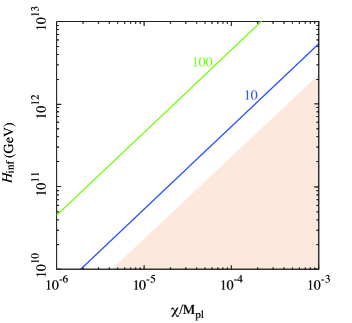
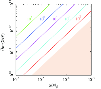
Figure 1: Contours of $f_{\rm NL}$ (left) and $g_{\rm NL}$ (right) in the $\chi$–$H_{\rm inf}$ plane for the Case I. $p=2$ is assumed. Shaded regions correspond to the parameter space where we cannot obtain the right amplitude for $P_{\zeta}$.

Case II: $\displaystyle\Gamma(\chi)=\Gamma_{0}\left[1+a\frac{\chi}{M}+b\left(\frac{\chi}{M}\right)^{2}\right]$.

In many models, the coupling can be written as a Taylor expansion of $\chi$, where $M$ represents some high energy scale and $\chi/M\ll 1$ is assumed. The coefficients $a$ and $b$ are parameters of order one, which are supposed to depend on the details of some explicit model of high energy physics. The non-linearity parameters are then given by

$$\tilde{f}_{\rm NL} = -\frac{12b}{a^{2}r}-r+\frac{9}{r}-2,$$ (35)

$$\tilde{g}_{\rm NL} = \frac{1}{r^{2}}\left[\frac{36b}{a^{2}}\left(r^{2}+2r-9\right)+3r^{4}+10r^{3}-22r^{2}-54r+135\right].$$ (36)

where we have used $\chi/M\ll 1$. As easily read off from the above expressions, the signs of $f_{\rm NL}$ and $g_{\rm NL}$ can be positive or negative, depending on $a$ and $b$. Since $a$ and $b$ are assumed to be $\mathcal{O}(1)$, the amplitude of $f_{\rm NL}$ and $g_{\rm NL}$ is mainly controlled by the value of $r$.

Case III: $\displaystyle\Gamma(\chi)=\Gamma_{0}\left[1+\left(\frac{\chi}{M}\right)^{q}\right]$ ($q\geq 2$).

In the latter case, we consider the possibility that the expansion starts with a higher order polynomial. Once again, $M$ is some high energy scale characterizing the underlying physics, and we assume $\chi/M\ll 1$. The non-linearity parameters are now given by

$$\frac{6}{5}f_{\rm NL} = -\frac{6}{r}\frac{q-1}{q}\left(\frac{M}{\chi}\right)^{q}-r+\frac{9}{r}-2,$$ (37)

$$\frac{54}{25}g_{\rm NL} = \frac{1}{r^{2}}\left[36\frac{(q-1)(q-2)}{q^{2}}\left(\frac{M}{\chi}\right)^{2q}+18\left(r^{2}+2r-9\right)\frac{q-1}{q}\left(\frac{M}{\chi}\right)^{q}\right.$$ (38)

$$\left.+\left(3r^{4}+10r^{3}-22r^{2}-54r+135\right)\right].$$

Since $\chi/M\ll 1$, one sees that $f_{\rm NL}$ can be large even with $r=1$, but the sign of $f_{\rm NL}$ is then negative, which is in contradiction with the current constraints from WMAP [2]. On the other hand, when $r\ll 1$, $f_{\rm NL}$ and $g_{\rm NL}$ can be both positive, which is similar to the case I.

4 Hybrid curvaton-modulaton case

In this section, we consider the general situation where both the curvaton and modulaton fluctuations contribute to the final density perturbation. We also take into account the inflaton contribution in the power spectrum.

The curvature perturbation in this case is given by (2), with the substitutions of (12). This leads to an expression of the form (18), which contains now three scalar fields $\phi$, $\sigma$ and $\chi$. It is convenient to introduce two dimensionless parameters that characterize the relative contributions of $\sigma$ and $\chi$ to the total power spectrum, defined by

$$\Xi_{\sigma}\equiv\frac{N_{\sigma}^{2}}{N_{\phi}^{2}+N_{\sigma}^{2}+N_{\chi}^{2}},\qquad\qquad\Xi_{\chi}\equiv\frac{N_{\chi}^{2}}{N_{\phi}^{2}+N_{\sigma}^{2}+N_{\chi}^{2}}.$$ (39)

The inflaton contribution in the power spectrum is thus given by $1-\Xi_{\sigma}-\Xi_{\chi}$.

The bispectrum parameter $\tilde{f}_{\rm NL}$ can then be decomposed into three terms (the inflaton does not contribute to the non-Gaussianity here)

$$\tilde{f}_{\rm NL} = \Xi_{\sigma}^{2}\,\tilde{f}_{\rm NL}^{(\sigma^{2})}+2\,\Xi_{\sigma}\,\Xi_{\chi}\,\tilde{f}_{\rm NL}^{(\sigma\chi)}+\Xi_{\chi}^{2}\,f_{\rm NL}^{(\chi^{2})},$$ (40)

where we have defined

$$\tilde{f}_{\rm NL}^{(\sigma^{2})}=\frac{N_{\sigma\sigma}}{N_{\sigma}^{2}},\qquad\tilde{f}_{\rm NL}^{(\sigma\chi)}=\frac{N_{\sigma\chi}}{N_{\sigma}N_{\chi}},\qquad\tilde{f}_{\rm NL}^{(\chi^{2})}=\frac{N_{\chi\chi}}{N_{\chi}^{2}}\,.$$

Their explicit expressions are

$$\tilde{f}_{\rm NL}^{(\sigma^{2})} = \frac{3}{2r}-2-r,$$ (41)

$$\tilde{f}_{\rm NL}^{(\chi^{2})} = -\frac{6}{r}\frac{\Gamma\Gamma^{\prime\prime}}{\Gamma^{{}^{\prime}2}}-r+\frac{9}{r}-2,$$ (42)

$$\tilde{f}_{\rm NL}^{(\sigma\chi)} = -r+\frac{3}{r}-2,$$ (43)

where the first equation corresponds to the standard curvaton expression[39], while the second one is the modulaton contribution calculated in the previous section. The final one is a mixed contribution.

Similarly, the trispectrum coefficient $\tilde{g}_{\rm NL}$ can be decomposed into four terms:

$$\tilde{g}_{\rm NL} = \Xi_{\sigma}^{3}\,\tilde{g}_{\rm NL}^{(\sigma^{3})}+3\,\Xi_{\sigma}^{2}\,\Xi_{\chi}\,\tilde{g}_{\rm NL}^{(\sigma^{2}\chi)}+3\,\Xi_{\sigma}\,\Xi_{\chi}^{2}\,\tilde{g}_{\rm NL}^{(\sigma\chi^{2})}+\Xi_{\chi}^{3}\,g_{\rm NL}^{(\chi^{3})},$$ (44)

where

$$\tilde{g}_{\rm NL}^{(\sigma^{3})}=\frac{N_{\sigma\sigma\sigma}}{N_{\sigma}^{3}},\qquad\tilde{g}_{\rm NL}^{(\sigma^{2}\chi)}=\frac{N_{\sigma\sigma\chi}}{N_{\sigma}^{2}N_{\chi}},\qquad\tilde{g}_{\rm NL}^{(\sigma\chi^{2})}=\frac{N_{\chi\chi\sigma}}{N_{\sigma}N_{\chi}^{2}},\qquad\tilde{g}_{\rm NL}^{(\chi^{3})}=\frac{N_{\chi\chi\chi}}{N_{\chi}^{3}}.$$ (45)

By using (2) and (12), we can explicitly write down these quantities as

$$\tilde{g}_{\rm NL}^{(\sigma^{3})} = 3r^{2}+10r-\frac{9}{r}+\frac{1}{2},$$ (46)

$$\tilde{g}_{\rm NL}^{(\sigma^{2}\chi)} = 3r^{2}+\frac{9}{2r^{2}}+10r-\frac{15}{r}-\frac{5}{2},$$ (47)

$$\tilde{g}_{\rm NL}^{(\sigma\chi^{2})} = \frac{1}{r^{2}}\left(r^{2}+2r-3\right)(\left(3r^{2}+4r-9\right)+\frac{6}{r^{2}}\left(r^{2}+2r-3\right)\frac{\Gamma\Gamma^{{}^{\prime\prime}}}{\Gamma^{\prime 2}},$$ (48)

$$\tilde{g}_{\rm NL}^{(\chi^{3})} = \frac{1}{r^{2}}\left[36\frac{\Gamma^{2}\Gamma^{{}^{\prime\prime\prime}}}{\Gamma^{\prime 3}}+18\left(r^{2}+2r-9\right)\frac{\Gamma\Gamma^{\prime\prime}}{\Gamma^{\prime 2}}+\left(3r^{4}+10r^{3}-22r^{2}-54r+135\right)\right],$$ (49)

where one can identify the usual curvaton contribution[43], the pure modulaton contribution calculated in the previous section, as well as two mixed curvaton-modulaton contributions.

Finally, the $\tau_{\rm NL}$ coefficient can be decomposed as

$$\tau_{\rm NL} = \Xi_{\sigma}^{3}\left(\tilde{f}_{\rm NL}^{(\sigma^{2})}\right)^{2}+2\,\Xi_{\sigma}^{2}\,\Xi_{\chi}\,\tilde{f}_{\rm NL}^{(\sigma^{2})}\tilde{f}_{\rm NL}^{(\sigma\chi)}+\Xi_{\sigma}\,\Xi_{\chi}\left(\Xi_{\sigma}+\Xi_{\chi}\right)\left(\tilde{f}_{\rm NL}^{(\sigma\chi)}\right)^{2}$$ (51)

$$\qquad\qquad\qquad+2\,\Xi_{\sigma}\,\Xi_{\chi}^{2}\,\tilde{f}_{\rm NL}^{(\chi^{2})}\tilde{f}_{\rm NL}^{(\sigma\chi)}+\Xi_{\chi}^{3}\left(\tilde{f}_{\rm NL}^{(\chi^{2})}\right)^{2}\,.$$

In the $r\ll 1$ limit, one finds that the dominant terms for the non-Gaussianity coefficients are

$$\tilde{f}_{\rm NL}=\frac{1}{2r}\left(3\Xi_{\sigma}^{2}+12\Xi_{\sigma}\Xi_{\chi}+18\Xi_{\chi}^{2}-12\Xi_{\chi}^{2}\frac{\Gamma\Gamma^{\prime\prime}}{\Gamma^{\prime 2}}\right)+{\cal O}(1),$$ (52)

$$\tau_{\rm NL}=\frac{9}{4r^{2}}\left[\Xi_{\sigma}^{3}+8\Xi_{\sigma}^{2}\Xi_{\chi}+\Xi_{\chi}^{2}\Xi_{\sigma}\left(28-16\frac{\Gamma\Gamma^{{}^{\prime\prime}}}{\Gamma^{2}}\right)+\Xi_{\chi}^{3}\left(36-48\frac{\Gamma\Gamma^{{}^{\prime\prime}}}{\Gamma^{2}}+16\frac{\Gamma^{2}\Gamma^{{}^{\prime\prime}2}}{\Gamma^{{}^{\prime}4}}\right)\right]+{\cal O}\left({\frac{1}{r}}\right),$$ (53)

$$\tilde{g}_{\rm NL} = \frac{9\,\Xi_{\chi}}{2r^{2}}\left[3\left(6\Xi_{\sigma}\Xi_{\chi}+\Xi_{\sigma}^{2}+10\Xi_{\chi}^{2}\right)-12\Xi_{\chi}\left(\Xi_{\sigma}+3\Xi_{\chi}\right)\frac{\Gamma\Gamma^{\prime\prime}}{\Gamma^{\prime 2}}+8\Xi_{\chi}^{2}\frac{\Gamma^{2}\Gamma^{\prime\prime\prime}}{\Gamma^{\prime 3}}\right]+{\cal O}\left({\frac{1}{r}}\right).$$

Here it is interesting to notice that the leading term of $g_{\rm NL}$ vanishes when $\Xi_{\chi}=0$. Thus the enhancement by the factor of $1/r^{2}$ comes from the modulaton fluctuations, which is absent in the standard curvaton model. This property of the trispectrum could be useful to discriminate this model from other ones.

5 Summary

We have investigated the density perturbations in a scenario based on the modulated decay of the curvaton, where the curvature perturbation is generated via the modulation of the curvaton decay rate due to its dependence on another scalar field, called the modulaton $\chi$. We have paid special attention to non-Gaussianity, since it is potentially the best way to discriminate among various scenarios, and we have computed specifically the non-linearity parameters $f_{\rm NL}$ and $g_{\rm NL}$ in this class of models.

As discussed in Section 3, this model shares some similarities with the usual curvaton and modulated reheating models: the size of these parameters are mainly determined by $r$, which is similar to the curvaton model. On the other hand, the signs of these parameters highly depend on the functional form of $\Gamma(\chi)$, which is the same as usual modulated reheating model. However, the model also exhibits interesting predictions coming from a hybrid nature of this model. When the curvaton is a subdominant component of the Universe at its decay, the non-linearity parameters are related as $g_{\rm NL}\propto f_{\rm NL}^{2}$ where the proportionality factor depends on the functional form of $\Gamma(\chi)$. Thus this model generically predicts enhanced $g_{\rm NL}$, which is different from the standard curvaton and modulated reheating models, predicting $g_{\rm NL}\sim f_{\rm NL}$.

We have also investigated a more general case where fluctuations of the curvaton itself also contribute to density fluctuations. We have presented the formulas of the curvature perturbation up to the 3rd order, and the non-linearity parameters. The formulas given in such a case naturally also include the standard curvaton and modulated reheating models, which provides a unified treatment of those kind of models and their variants.

Although we have considered only adiabatic perturbations in the present work, the modulated decay of the curvaton could also produce isocurvature perturbations, similarly to the standard curvaton scenario[44]. It would be interesting to study these possible isocurvature modes and their non-Gaussianities following the analysis introduced in [45, 46]. Isocurvature modes, possibly correlated with adiabatic modes, lead to very specific signatures in the CMB non-Gaussianities and Planck or future CMB data could detect these isocurvature non-Gaussianities[47, 48].

In the near future, one can hope that new cosmological data of unprecedented precision, in particular from Planck, will enable to test the model presented here, together with various other mechanisms that generate primordial density perturbations. In this respect, the unified treatment proposed in this paper should be useful for a simplified confrontation of a large class of models with cosmological data.

Note added: While completing this manuscript, we became aware that the authors of [52] were working on a very similar topic.

References

- [1] D. Langlois, Lect. Notes Phys. 800, 1 (2010) [arXiv:1001.5259 [astro-ph.CO]].
- [2] C. L. Bennett, D. Larson, J. L. Weiland, N. Jarosik, G. Hinshaw, N. Odegard, K. M. Smith and R. S. Hill et al., arXiv:1212.5225 [astro-ph.CO].
- [3] J. -Q. Xia, M. Viel, C. Baccigalupi, G. De Zotti, S. Matarrese and L. Verde, Astrophys. J. 717, L17 (2010) [arXiv:1003.3451 [astro-ph.CO]].
- [4] K. Enqvist and M. S. Sloth, Nucl. Phys. B 626, 395 (2002) [arXiv:hep-ph/0109214].
- [5] D. H. Lyth and D. Wands, Phys. Lett. B 524, 5 (2002) [arXiv:hep-ph/0110002].
- [6] T. Moroi and T. Takahashi, Phys. Lett. B 522, 215 (2001) [Erratum-ibid. B 539, 303 (2002)] [arXiv:hep-ph/0110096].
- [7] G. Dvali, A. Gruzinov and M. Zaldarriaga, Phys. Rev. D 69, 023505 (2004) [arXiv:astro-ph/0303591].
- [8] L. Kofman, arXiv:astro-ph/0303614.
- [9] F. Bernardeau and J. -P. Uzan, Phys. Rev. D 67, 121301 (2003) [astro-ph/0209330].
- [10] F. Bernardeau, L. Kofman and J. -P. Uzan, Phys. Rev. D 70, 083004 (2004) [astro-ph/0403315].
- [11] D. H. Lyth, JCAP 0511, 006 (2005) [astro-ph/0510443].
- [12] M. P. Salem, Phys. Rev. D 72, 123516 (2005) [astro-ph/0511146].
- [13] D. Langlois and L. Sorbo, JCAP 0908, 014 (2009) [arXiv:0906.1813 [astro-ph.CO]].
- [14] D. Battefeld, T. Battefeld, C. Byrnes and D. Langlois, JCAP 1108, 025 (2011) [arXiv:1106.1891 [astro-ph.CO]].
- [15] D. Langlois and F. Vernizzi, Phys. Rev. D 70, 063522 (2004) [arXiv:astro-ph/0403258];
- [16] G. Lazarides, R. R. de Austri and R. Trotta, Phys. Rev. D 70, 123527 (2004) [hep-ph/0409335].
- [17] T. Moroi, T. Takahashi and Y. Toyoda, Phys. Rev. D 72, 023502 (2005) [arXiv:hep-ph/0501007];
- [18] T. Moroi and T. Takahashi, Phys. Rev. D 72, 023505 (2005) [arXiv:astro-ph/0505339];
- [19] K. Ichikawa, T. Suyama, T. Takahashi and M. Yamaguchi, Phys. Rev. D 78, 023513 (2008) [arXiv:0802.4138 [astro-ph]].
- [20] K. Ichikawa, T. Suyama, T. Takahashi and M. Yamaguchi, Phys. Rev. D 78, 063545 (2008) [arXiv:0807.3988 [astro-ph]].
- [21] K. Y. Choi and J. O. Gong, JCAP 0706, 007 (2007) [arXiv:0704.2939 [astro-ph]].
- [22] H. Assadullahi, J. Valiviita and D. Wands, Phys. Rev. D 76, 103003 (2007) [arXiv:0708.0223 [hep-ph]].
- [23] T. Suyama, T. Takahashi, M. Yamaguchi and S. Yokoyama, JCAP 1012, 030 (2010) [arXiv:1009.1979 [astro-ph.CO]].
- [24] K. -Y. Choi and O. Seto, Phys. Rev. D 85, 123528 (2012) [arXiv:1204.1419 [astro-ph.CO]].
- [25] K. Enqvist and S. Nurmi, JCAP 0510, 013 (2005) [astro-ph/0508573].
- [26] K. Enqvist and T. Takahashi, JCAP 0809, 012 (2008) [arXiv:0807.3069 [astro-ph]].
- [27] K. Enqvist, S. Nurmi, G. Rigopoulos, O. Taanila and T. Takahashi, JCAP 0911, 003 (2009) [arXiv:0906.3126 [astro-ph.CO]].
- [28] K. Enqvist and T. Takahashi, JCAP 0912, 001 (2009) [arXiv:0909.5362 [astro-ph.CO]].
- [29] K. Enqvist, S. Nurmi, O. Taanila and T. Takahashi, JCAP 1004, 009 (2010) [arXiv:0912.4657 [astro-ph.CO]].
- [30] K. Dimopoulos, D. H. Lyth, A. Notari and A. Riotto, JHEP 0307, 053 (2003) [hep-ph/0304050].
- [31] M. Kawasaki, K. Nakayama and F. Takahashi, JCAP 0901, 026 (2009) [arXiv:0810.1585 [hep-ph]].
- [32] P. Chingangbam and Q. G. Huang, JCAP 0904, 031 (2009) [arXiv:0902.2619 [astro-ph.CO]].
- [33] M. Kawasaki, T. Kobayashi and F. Takahashi, Phys. Rev. D 84, 123506 (2011) [arXiv:1107.6011 [astro-ph.CO]].
- [34] D. Langlois and T. Takahashi, in preparation.
- [35] D. H. Lyth, K. A. Malik and M. Sasaki, JCAP 0505, 004 (2005) [arXiv:astro-ph/0411220].
- [36] D. Langlois and F. Vernizzi, Phys. Rev. Lett. 95, 091303 (2005) [arXiv:astro-ph/0503416].
- [37] D. Langlois and F. Vernizzi, Phys. Rev. D 72, 103501 (2005) [arXiv:astro-ph/0509078].
- [38] D. Langlois and F. Vernizzi, Class. Quant. Grav. 27, 124007 (2010) [arXiv:1003.3270 [astro-ph.CO]].
- [39] D. H. Lyth and Y. Rodriguez, Phys. Rev. Lett. 95, 121302 (2005) [arXiv:astro-ph/0504045].
- [40] L. Alabidi and D. H. Lyth, JCAP 0605, 016 (2006) [arXiv:astro-ph/0510441].
- [41] C. T. Byrnes, M. Sasaki and D. Wands, Phys. Rev. D 74, 123519 (2006) [arXiv:astro-ph/0611075].
- [42] T. Suyama and M. Yamaguchi, Phys. Rev. D 77, 023505 (2008) [arXiv:0709.2545 [astro-ph]].
- [43] M. Sasaki, J. Valiviita and D. Wands, Phys. Rev. D 74, 103003 (2006) [astro-ph/0607627].
- [44] D. H. Lyth, C. Ungarelli and D. Wands, Phys. Rev. D 67, 023503 (2003) [astro-ph/0208055].
- [45] D. Langlois and A. Lepidi, JCAP 1101, 008 (2011) [arXiv:1007.5498 [astro-ph.CO]].
- [46] D. Langlois and T. Takahashi, JCAP 1102, 020 (2011) [arXiv:1012.4885 [astro-ph.CO]].
- [47] D. Langlois and B. van Tent, Class. Quant. Grav. 28, 222001 (2011) [arXiv:1104.2567 [astro-ph.CO]].
- [48] D. Langlois and B. van Tent, JCAP 1207, 040 (2012) [arXiv:1204.5042 [astro-ph.CO]].
- [49] C. Hikage, K. Koyama, T. Matsubara, T. Takahashi and M. Yamaguchi, Mon. Not. Roy. Astron. Soc. 398, 2188 (2009) [arXiv:0812.3500 [astro-ph]].
- [50] C. Hikage, M. Kawasaki, T. Sekiguchi and T. Takahashi, arXiv:1211.1095 [astro-ph.CO].
- [51] C. Hikage, M. Kawasaki, T. Sekiguchi and T. Takahashi, arXiv:1212.6001 [astro-ph.CO].
- [52] H. Assadullahi, H. Firouzjahi, M. H. Namjoo and D. Wands, to appear.