Double scale analysis of periodic solutions of some non linear vibrating systems

Abstract

We consider small solutions of a vibrating system with smooth non-linearities for which we provide an approximate solution by using a double scale analysis; a rigorous proof of convergence of a double scale expansion is included; for the forced response, a stability result is needed in order to prove convergence in a neighbourhood of a primary resonance. Keywords: double scale analysis; periodic solutions; nonlinear vibrations, resonance MSC: 34e13, 34c25, 74h10, 74h45

1 Introduction

In this work we look for an asymptotic expansion of small periodic solutions of free vibrations of a discrete structure without damping and with local non linearity; then the same system with light damping and a periodic forcing with frequency close to a frequency of the free system is analyzed (primary resonance). For a small solution, we recover a behavior with some similarity with the linear case; in particular the amplitude of the forced response reaches a local maximum at the frequency of the free response. On the other hand the frequency of the free response is amplitude dependent and the superposition principle does not apply. The work of Lyapunov [oL49] is often cited as a basis for the existence of periodic solutions which tends towards linear normal modes as amplitudes tend to zero; the proof of this paper uses the hypothesis of analycity of the non linearity involved in the differential system. In [Rou11], we addressed the case of a non linearity which is only lipschitzian and we prove existence of periodic solutions with a constructive proof; in this case the result of Lyapunov obviously may not be applied. Non-linearity of oscillations is a classical theme in theoretical physics, for example at master level, see [LL58] in Russian or its English or French translation in [LL60, LL66].

Asymptotic expansions have been used for a long time; such methods are introduced in the famous memoir of Poincaré [Poi99]; a general book on asymptotic methods is [BM55] with french and English translations [BM62, BM61]; introductory material is in [Nay81], [Mil06]; a detailed account of the averaging method with precise proofs of convergence may be found in [SV85]; an analysis of several methods including multiple scale expansion may be found in [Mur91]; the case of vibrations with unilateral springs have been presented in [JR09, JR10, VLP08], [HR09a, HR09b, HFR09, Haz, Haz10]; in [JPS04] a numerical approach for large solutions of piecewise linear systems is proposed. The case of rigid contact which is also important from the point of view of theory and applications has been addressed in several papers, for example [JL01], and a synthesis in [JBL13] . A review paper for so called “non linear normal modes” may be found in [KPGV09]; it includes numerous papers published by the mechanical community; several application fields have been addressed by the mechanical community; for example in [Mik10] “nonlinear vibro-absorption problem, the cylindrical shell nonlinear dynamics and the vehicle suspension nonlinear dynamics are analyzed”.

In the mechanical engineering community the validity of the expansions is assumed to hold; however, this is not straightforward as this kind of expansion is not a standard series expansion and the expansion is usually not valid for all time; for example, this point has been raised in [Rub78]. If the averaging method was carefully analyzed as indicated above, it seems not to be the case for the multiple scale method, the expansion of which is often compared to the one obtained by the averaging method.

Here in a first stage we consider small solutions of a system with smooth non-linearities for which we provide an approximate solution by using a double scale analysis; a rigorous proof of convergence of the method of double scale is included; for the forced response, a stability result is needed in order to prove convergence. As an introduction, the next section addresses the one degree of freedom case while the following one considers many degrees of freedom; for free vibrations we find solutions close to a linear normal mode (so called non linear normal modes) and for forced vibrations, we describe the response for forcing frequency close to a free vibration frequency. Preliminary versions of these results may be found in [BR09] and have been presented in conferences [Bra10, Bra]; related results have been presented in [Gas]. Triple scale expansions is to be submitted [BR13]. In a forthcoming paper, the non-smooth case will be considered as well as a numerical algorithm based on the fixed point method used in [Rou11].

2 One degree of freedom, strong cubic non linearity

In this section, we consider the case of a mass attached to a spring; in the case of a stress-strain law of the form ${n}{}=ku+mcu^{2}+mu^{3}$, we find no shift of frequency at first order, so here we concentrate on a stress-strain law with a stronger cubic non linearity:

$${n}{}=ku+mcu^{2}+m\frac{d}{\epsilon}u^{3}$$

where $\epsilon$ is a small parameter which is also involved in the size of the solution as in previous paragraph; the choice of this scaling provides frequencies which are amplitude dependent.

2.1 Free vibration, double scale expansion up to first order

Using second Newton law, free vibrations of a mass attached to such a spring are governed by:

$$\ddot{u}+\omega^{2}u+cu^{2}+\frac{du^{3}}{\epsilon}=0.$$ (1)

We look for a small solution with a double scale for time; we set

$$T_{0}=\omega t,\quad T_{1}=\epsilon t,$$ (2)

so with $D_{0}u=\frac{\partial u}{\partial T_{0}},\quad D_{1}u=\frac{\partial u}{\partial T_{1}}$, we obtain

$$\frac{du}{dt}=\omega D_{0}u+\epsilon D_{1}u,\;\frac{d^{2}u}{dt^{2}}=\omega^{2}D^{2}_{0}u+2\epsilon\omega D_{0}D_{1}u+\epsilon^{2}D_{1}^{2}u$$ (3)

and we look for a small solution with initial data

$u(0)=\epsilon a_{0}+o(\epsilon)$ and $\dot{u}(0)=o(\epsilon)$; we use the ansatz

$$u=\epsilon u_{1}(T_{0},T_{1})+\epsilon^{2}r(T_{0},T_{1},\epsilon);$$ (4)

so we have:

$$\frac{du}{dt}=\epsilon[\omega D_{0}u_{1}+\epsilon D_{1}u_{1}]+\epsilon^{2}[\omega D_{0}r+\epsilon D_{1}r]$$ (5)

and

$$\frac{d^{2}u}{dt^{2}}=\epsilon\omega^{2}D^{2}_{0}u_{1}+\epsilon^{2}[2\omega D_{0}D_{1}u_{1}+\omega^{2}D_{0}^{2}r]+\epsilon^{3}[D_{1}^{2}u_{1}+\mathcal{D}_{2}r]$$ (6)

with

$$\mathcal{D}_{2}r=\frac{1}{\epsilon}\left(\frac{d^{2}r}{dt^{2}}-\omega^{2}D_{0}^{2}r\right)=2\omega D_{0}D_{1}r+\epsilon D_{1}^{2}r$$ (7)

We plug expansions (4),(6) into (1); by identifying the powers of $\epsilon$ in the expansion of equation (1), we obtain:

$$\Bigg{\{}\begin{array}[h]{rl}&\omega^{2}(D_{0}^{2}u_{1}+u_{1})=0\\ &(D_{0}^{2}r+r)=\frac{S_{2}}{\omega^{2}}\quad\text{ with }\\ \end{array}$$ (10)

$$S_{2}=-\frac{1}{\epsilon^{2}}\left[c(\epsilon u_{1}+\epsilon^{2}r)^{2}+\frac{d}{\epsilon}(\epsilon u_{1}+\epsilon^{2}r)^{3}\right]-2\omega D_{0}D_{1}u_{1}-\epsilon{\cal R}(u_{1},r,\epsilon)$$ (11)

where

$${\cal R}=D_{1}^{2}u_{1}+{\cal D}_{2}r;$$ (12)

we can manipulate to obtain:

$$S_{2}=-\left[cu_{1}^{2}+du_{1}^{3}+2\omega D_{0}D_{1}u_{1}+\epsilon R(u_{1},r,\epsilon)\right]$$ (13)

where

$$R(u_{1},r,\epsilon)=\left[{\cal R}+2cu_{1}r+3du_{1}^{2}r+\epsilon\rho(u_{1},r,\epsilon)\right]$$ (14)

with a polynomial $\rho(u_{1},r,\epsilon)=cr^{2}+3du_{1}r^{2}+\epsilon dr^{3}$ .

We set $\theta(T_{0},T_{1})=T_{0}+\beta(T_{1})$ noticing $D_{0}\theta=1,\;D_{1}\theta=D_{1}\beta$; we solve equation (10) with:

$$u_{1}=a(T_{1})\cos(\theta)$$ (15)

and we obtain

$$S_{2}=\frac{-ca^{2}}{2}(1+\cos(2\theta))-\frac{da^{3}}{4}\left(\cos(3\theta)+3\cos(\theta)\right)+\\ 2\omega(D_{1}a\sin(\theta)+aD_{1}\beta\cos(\theta))-\epsilon R(u_{1},r,\epsilon);$$ (16)

we gather terms at angular frequency $1$:

$$S_{2}=-\frac{da^{3}}{4}3\cos(\theta)+2\omega\left[D_{1}a\sin(\theta)+aD_{1}\beta\cos(\theta)\right]+S_{2}^{\sharp}-\epsilon R(u_{1},r,\epsilon)$$ (17)

where

$$S_{2}^{\sharp}=\frac{-ca^{2}}{2}(1+\cos(2\theta))-\frac{da^{3}}{4}\cos(3\theta).$$ (18)

By imposing

$$D_{1}a=0\text{ and }\quad 2\omega aD_{1}\beta=3\frac{da^{3}}{4},\text{ so that }\\ a=a_{0},\quad\beta=\beta_{0}T_{1}\text{ with }\beta_{0}=3\frac{da^{2}}{8\omega}T_{1},$$ (19)

we get that $S_{2}=S_{2}^{\sharp}-\epsilon R(u_{1},r,\epsilon)$ no longer contains any term at frequency $1$.

In order to show that $r$ is bounded, after eliminating terms at angular frequency $1$, we go back to the $t$ variable in the second equation (10).

$$\ddot{r}+\omega^{2}r=\frac{\tilde{S_{2}}}{\omega^{2}}\quad\text{ with }$$ (20)

$$\tilde{S_{2}}=S_{2}^{\sharp}(t,\epsilon)-\epsilon\tilde{R}(u_{1},r,\epsilon)\text{ where }$$ (21)

$$S_{2}^{\sharp}(t,\epsilon)=\frac{-ca^{2}}{2}\left[1+\cos(2(\omega t+\beta(\epsilon t)))\right]-\frac{da^{3}}{4}\cos(3(\omega t+\beta(\epsilon t)))$$ (22)

$$\quad\quad=\frac{-ca^{2}}{2}(1+\cos(2(\omega t+\beta_{0}\epsilon t))-\frac{da^{3}}{4}\left(\cos(3(\omega t+\beta_{0}\epsilon t))\right)$$ (23)

$$\text{ with }\tilde{R}(u_{1},r,\epsilon)=R(u_{1},r,\epsilon)-\mathcal{D}_{2}r$$ (24)

in which the remainder $\tilde{R}$ is expressed with variable $t$.

Proposition 2.1.

There exists $\gamma>0$ such that for all $t\leq t_{\epsilon}=\frac{\gamma}{\epsilon}$, the solution of (1), with $u(0)=\epsilon a_{0}+o(\epsilon),~{}\dot{u}(0)=o(\epsilon)$, satisfies the following expansion

$$u(t)=\epsilon a_{0}~{}\cos(\nu_{\epsilon}t)~{}+~{}\epsilon^{2}r(\epsilon,t)$$

where

$$\nu_{\epsilon}=\omega+3\epsilon\frac{da^{2}}{8{\omega}}$$ (25)

and $r$ is uniformly bounded in $C^{2}(0,t_{\epsilon})$ .

Proof.

Let us use lemma 5.1 with equation (20); set $S=S_{2}^{\sharp}$; as we have enforced (19), it is a periodic bounded function orthogonal to $e^{\pm it}$, it satisfies lemma hypothesis; similarly set $g=\tilde{R}$; it is a polynomial in variable $r$ with coefficients which are bounded functions, so it is a lipschitzian function on bounded subsets and satisfies lemma hypothesis. ∎

2.2 Forced vibration, double scale expansion of order 1

2.2.1 Derivation of the expansion

Here we consider a similar system with a sinusoidal forcing at a frequency close to the free frequency (so called primary resonance); in the linear case, without damping, it is well known that the solution is no longer bounded when the forcing frequency goes to the free frequency. Here, we consider the mechanical system of previous section but with periodic forcing and we include some light damping term; the scaling of the forcing term is chosen so that the expansion works properly; this is a known difficulty, for example see [Nay86].

$$\ddot{u}+\omega^{2}u+\epsilon\lambda\dot{u}+cu^{2}+\frac{du^{3}}{\epsilon}=\epsilon^{2}F\cos(\tilde{\omega}_{\epsilon}t).$$ (26)

We assume positive damping, $\lambda>0$ and excitation frequency $\tilde{\omega}_{\epsilon}$ is close to an eigenfrequency of the linear system in the following way:

$$\tilde{\omega}_{\epsilon}=\omega+\epsilon\sigma.$$ (27)

We look for a small solution with a double scale expansion; to simplify the computations, the fast scale $T_{0}$ is chosen $\epsilon$ dependent and we set:

$$T_{0}=\tilde{\omega}_{\epsilon}t,\quad T_{1}=\epsilon t\text{ and }\quad D_{0}u=\frac{\partial u}{\partial T_{0}},~{}D_{1}u=\frac{\partial u}{\partial T_{1}};$$ (28)

so

$$\frac{du}{dt}=\tilde{\omega}D_{0}u+\epsilon D_{1}u\;\text{ and }\;\frac{d^{2}u}{dt^{2}}=\tilde{\omega}_{\epsilon}^{2}D^{2}_{0}u+2\epsilon\tilde{\omega}_{\epsilon}D_{0}D_{1}u+\epsilon^{2}D_{1}^{2}u;$$ (29)

equation (27) provides

$$\tilde{\omega}_{\epsilon}^{2}=\omega^{2}+2\epsilon\omega\sigma+\epsilon^{2}\sigma^{2}.$$ (30)

With (27), (28), (29), (30) and the ansatz

$$u=\epsilon u_{1}(T_{0},T_{1})+\epsilon^{2}r(T_{0},T_{1},\epsilon),$$ (31)

we obtain:

$$\frac{du}{dt}=\epsilon\frac{du_{1}}{dt}+\epsilon^{2}\frac{dr}{dt}=\epsilon\frac{du_{1}}{dt}+\epsilon^{2}\omega D_{0}r+\epsilon^{2}(\frac{dr}{dt}-\omega D_{0}r)=$$ (32)

$$\epsilon[\tilde{\omega}D_{0}u_{1}+\epsilon D_{1}u_{1}]+\epsilon^{2}\omega D_{0}r+\epsilon^{2}(\frac{dr}{dt}-\omega D_{0}r)=$$ (33)

$$\epsilon[\omega D_{0}u_{1}+\epsilon\sigma D_{0}u_{1}+\epsilon D_{1}u_{1}]+\epsilon^{2}\omega D_{0}r+\epsilon^{2}(\frac{dr}{dt}-\omega D_{0}r)$$ (34)

where we remark that $\frac{dr}{dt}-\omega D_{0}r=\epsilon\sigma D_{0}r+\epsilon D_{1}r$ is of degree 1 in $\epsilon$. For the second derivative, as for the case without forcing, we introduce

$${\cal D}_{2}r =\frac{1}{\epsilon}\left(\frac{d^{2}r}{dt^{2}}-\omega^{2}D_{0}^{2}r\right)\text{ with the expansion}$$ (35)

$${\cal D}_{2}r =2\omega[\sigma D_{0}^{2}r+D_{0}D_{1}r]+\epsilon\left[\sigma^{2}D_{0}^{2}r+2\sigma D_{0}D_{1}r+D_{1}^{2}r\right];$$ (36)

$$\frac{d^{2}u}{dt^{2}} =\epsilon\frac{d^{2}u_{1}}{dt^{2}}+\epsilon^{2}\frac{d^{2}r}{dt^{2}}=\epsilon\frac{d^{2}u_{1}}{dt^{2}}+\epsilon^{2}\omega^{2}D_{0}^{2}r+\epsilon^{3}{\cal D}_{2}r$$ (37)

$$=\epsilon\left[\tilde{\omega}^{2}D^{2}_{0}u_{1}+2\epsilon\tilde{\omega}D_{0}D_{1}u_{1}+\epsilon^{2}D_{1}^{2}u_{1}\right]$$ (38)

$$\qquad\qquad\qquad+\epsilon^{2}\omega^{2}D_{0}^{2}r+\epsilon^{3}{\cal D}_{2}r$$ (39)

$$=\epsilon\big{\{}\omega^{2}D^{2}_{0}u_{1}+2\epsilon\omega\left(\sigma D_{0}^{2}u_{1}+D_{0}D_{1}u_{1}\right)+$$ (40)

$$\qquad\qquad\qquad\epsilon^{2}\left[\sigma^{2}D_{0}^{2}u_{1}+2\sigma D_{0}D_{1}u_{1}+D_{1}^{2}u_{1}\right]\big{\}}$$ (41)

$$\qquad\qquad\qquad\qquad\qquad+\epsilon^{2}\omega^{2}D_{0}^{2}r+\epsilon^{3}{\cal D}_{2}r$$ (42)

the last term in the right hand side will be part of the remainder $R$ of equation (46). We plug previous expansions into (26); we obtain:

$$\Bigg{\{}\begin{array}[]{rl}&\omega^{2}(D_{0}^{2}u_{1}+u_{1})=0\\ &D_{0}^{2}r+r=\frac{S_{2}}{\omega^{2}}\quad\text{ with}\end{array}$$ (45)

$$S_{2}=-\left\{cu_{1}^{2}+du_{1}^{3}+2\omega[D_{0}D_{1}u_{1}+\sigma D_{0}^{2}u_{1}]+\lambda\omega D_{0}u_{1}\right\}$$ (46)

$$+F\cos(T_{0})-\epsilon R(u_{1},r,\epsilon)$$ (47)

and with

$$R(u_{1},r,\epsilon)=D_{1}^{2}u_{1}+2cu_{1}r+3du_{1}^{2}r+\sigma^{2}D_{0}^{2}u_{1}+2\sigma D_{0}D_{1}u_{1}+$$ (48)

$$\lambda(\omega D_{0}r+\sigma D_{0}u_{1}+D_{1}u_{1})+{\cal D}_{2}r$$ (49)

$$+\lambda(\frac{dr}{dt}-\omega D_{0}r)+\epsilon\rho(u_{1},r,\epsilon).$$ (50)

Set $\theta(T_{0},T_{1})=T_{0}+\beta(T_{1})$. We solve the first equation of (45) :

$$u_{1}=a(T_{1})\cos(\theta);$$ (51)

then we use $T_{0}=\theta(T_{0},T_{1})-\beta(T_{1})$ and we obtain

$$S_{2}=\frac{-ca^{2}}{2}(1+\cos(2\theta))-\frac{da^{3}}{4}\left(\cos(3\theta)+3\cos(\theta)\right)+\\ 2\omega(D_{1}a\sin(\theta)+aD_{1}\beta\cos(\theta))+2\sigma\omega a\cos(\theta)+a\lambda\omega\sin(\theta)\\ +F\sin(\theta)\sin(\beta(T_{1}))+F\cos(\theta)\cos(\beta(T_{1}))-\epsilon R(u_{1},r,\epsilon)$$ (52)

or

$$S_{2}=\left[2\omega D_{1}a+\lambda a\omega+F\sin(\beta)\right]\sin(\theta)\\ +\left[2\omega aD_{1}\beta+2\sigma\omega a-\frac{3da^{3}}{4}+F\cos(\beta)\right]\cos(\theta)\\ +S_{2}^{\sharp}~{}\quad-\epsilon R(u_{1},r,\epsilon)$$ (53)

with

$$S_{2}^{\sharp}=\frac{-ca^{2}}{2}(1+\cos(2\theta))-\frac{da^{3}}{4}\left(\cos(3\theta)\right);$$ (54)

note that $S_{2}^{\sharp}$ is a periodic function with frequency strictly multiple of $1$.

Orientation.

By enforcing

$$\Bigg{\{}\begin{array}[h]{rl}&2\omega D_{1}a+\lambda a\omega=-F\sin(\beta)\\ &2a\omega D_{1}\beta+2\sigma\omega a-\frac{3da^{3}}{4}=-F\cos(\beta)\end{array}$$ (57)

$S_{2}=S_{2}^{\sharp}-\epsilon R(u_{1},r,\epsilon)$ contains neither term at frequency $1$ nor at a frequency which goes to $1$; this point will enable to justify this expansion under some conditions; before, we study stationary solution of this system and the stability of the dynamic solution in a neighborhood of the stationary solution.

2.2.2 Stationary solution and stability

Let us consider the stationary solution of (57), it satisfies:

$$\Bigg{\{}\begin{array}[h]{rl}\lambda a\omega&+F\sin(\beta)=0\\ \left(2\omega\sigma-\frac{3da^{2}}{4}\right)&+\frac{F\cos(\beta)}{a}=0.\end{array}$$ (60)

Now, we study the stability of the solution of (57), in a neighborhood of this stationary solution noted $(\bar{a},\bar{\beta})$; set $a=\bar{a}+\tilde{a},\beta=\bar{\beta}+\tilde{\beta}$, the linearized system is written

$$\binom{D_{1}\tilde{a}}{D_{1}\tilde{\beta}}=J\binom{\tilde{a}}{\tilde{\beta}};$$

manipulating, we obtain the jacobian matrix.

$$J=\begin{pmatrix}-\frac{\lambda}{2}&-\frac{F}{2\omega}\cos(\bar{\beta})\\ \frac{9d\bar{a}}{8\omega}-\frac{\sigma}{\bar{a}}&\frac{F}{2\omega\bar{a}}\sin(\bar{\beta})\end{pmatrix}=\begin{pmatrix}-\frac{\lambda}{2}&a(\sigma-\frac{3d\bar{a}^{2}}{8\omega})\\ \frac{9d\bar{a}}{8\omega}-\frac{\sigma}{\bar{a}}&-\frac{\lambda}{2}\end{pmatrix}.$$ (61)

The matrix trace is $-\lambda$, and the determinant is

$$det(J)=\frac{\lambda^{2}}{4}-(\frac{9d\bar{a}^{2}}{8\omega}-\sigma)(\sigma-\frac{3d\bar{a}^{2}}{8\omega};)$$

we notice that the determinant is strictly positive for $\sigma=0$ so by continuity, it remains positive for $\sigma$ small; moreover $\frac{d}{d\sigma}det(J)<0$ for $\sigma<0$ so $det(J)>0$ for $\sigma<0$; by studying the trinomial in $\sigma$, we notice that the determinant is positive when this semi-implicit inequality is satisfied: $\sigma\leq\frac{3d\bar{a}^{2}}{4\omega}-\frac{1}{2}\sqrt{\frac{9d^{2}\bar{a}^{4}}{16\omega^{2}}-\lambda^{2}}$; so in these conditions, the two eigenvalues are negative; then the solution of the linearized system goes to zero; with the theorem of Poincaré-Lyapunov (look in the appendix for the theorem 5.1,) when the initial data is close enough to the stationary solution, the solution of the system (57), goes to the stationary solution. We expand this point, set

$$y=\binom{a}{\beta},\quad G(y)=\left(\begin{array}[h]{rl}-\lambda a\omega&-F\sin(\beta)\\ -\left(2\omega\sigma-\frac{3da^{2}}{4}\right)&-\frac{F\cos(\beta)}{a}\end{array}\right);$$ (62)

the system (60) may be written $\dot{y}=G(y)$; denote $\bar{y}=\binom{\bar{a}}{\bar{\beta}}$ the solution of (60); perform the change of variable $y=\bar{y}+x$, we have $G(\bar{y}+x)=G(\bar{y})+Jx+g(x)$ with $g(x)=o(\|x\|$; the theorem 5.1 may be applied with $A=J,\;B=0$, here the function $g$ does not depends on time.

Proposition 2.2.

If $\sigma\leq\frac{3d\bar{a}^{2}}{4\omega}-\frac{1}{2}\sqrt{\frac{9d^{2}\bar{a}^{4}}{16\omega^{2}}-\lambda^{2}}$ , the stationary solution of (57) is stable in the sense of Lyapunov (if the dynamic solution starts close to the stationary solution of (60), it remains close to it and converges to it ); to the stationary case corresponds the approximate solution of (26) $u_{1}=\bar{a}\cos(T_{0}+\bar{\beta})$, it is periodic; for an initial data close enough to this stationary solution, $u_{1}=a(T_{1})\cos(T_{0}+\beta(T_{1}))$ with $a,\beta$ solutions of (57); it goes to the solution (60) $\bar{a},\bar{\beta}$ when $T_{1}\longrightarrow+\infty$.

With this result of stability, we can state precisely the approximation of the solution of (26) by the function $u_{1}$.

2.2.3 Convergence of the expansion

Proposition 2.3.

Consider the solution of (26) with

$$u(0)=\epsilon a_{0}+o(\epsilon),~{}\dot{u}(0)=-\epsilon\omega a_{0}\sin(\beta_{0})+o(\epsilon),$$

with $a_{0},\beta_{0}$ close of the stationary solution $(\bar{a},\bar{\beta})$,

$$|a_{0}-\bar{a}|\leq\epsilon C_{1},|\beta_{0}-\bar{\beta}|\leq\epsilon C_{2};$$

When $\sigma\leq\frac{3d\bar{a}^{2}}{4\omega}-\frac{1}{2}\sqrt{\frac{3d\bar{a}^{2}}{2\omega}-\lambda^{2}}$, there exists $\gamma>0$ such that for all $t\leq t_{\epsilon}=\frac{\gamma}{\epsilon}$, the following expansion is satisfied

$$u(t)=\epsilon a(\epsilon t)~{}\cos(\tilde{\omega}_{\epsilon}t+\beta(\epsilon t))~{}+~{}\epsilon^{2}r(\epsilon,t)$$

with $\omega_{\epsilon}=\omega+\epsilon\sigma$ and $r$ uniformly bounded in $C^{2}(0,t_{\epsilon})$ and with $a,~{}\beta$ solution of (57).

Proof.

Indeed after eliminating terms at frequency $1$, we go back to the variable $t$ for the second equation (45)

$$\ddot{r}+\omega^{2}r=\frac{\tilde{S_{2}}}{\omega^{2}}\text{ with }$$ (63)

$$\tilde{S_{2}}=S_{2}^{\sharp}(t,\epsilon)-\epsilon\tilde{R}(u_{1},r,\epsilon)$$ (64)

where

$$\tilde{R}(u_{1},r,\epsilon)=R(u_{1},r,\epsilon)-{\cal D}_{2}r-\lambda(\frac{dr}{dt}-\omega D_{0}r)$$ (65)

with all the terms expressed with the variable $t$; we have

$$S_{2}^{\sharp}(t,\epsilon)=\frac{-ca^{2}(\epsilon t)}{2}(1+\cos(2(\tilde{\omega}_{\epsilon}t+\beta(\epsilon t)))-\frac{da^{3}(\epsilon t)}{4}\left(\cos(3(\tilde{\omega}_{\epsilon}t+\beta(\epsilon t)\right);$$ (66)

this function is not periodic but is close of the periodic function:

$$S_{2}^{\natural}(t,\epsilon)=\frac{-c\bar{a}^{2}}{2}(1+\cos(2(\tilde{\omega}_{\epsilon}t+\bar{\beta}))-\frac{da^{3}}{4}\left(\cos(3(\tilde{\omega}_{\epsilon}t+\bar{\beta})\right)$$ (67)

and for $t\leq\frac{\gamma}{\epsilon}$ as the solution of (57) is stable: it remains close to the stationary solution

$$|a(\epsilon t)-\bar{a}|\leq\epsilon C_{1},\quad|\beta(\epsilon t)-\bar{\beta}|\leq\epsilon C_{2}$$ (68)

and

$$|S_{2}^{\sharp}-S_{2}^{\natural}|\leq\epsilon C_{3};$$ (69)

so this difference may be included in the remainder $\tilde{R}$. We use lemma 5.1 with $S=S_{2}^{\natural}$; it satisfies lemma hypothesis; similarly, we use $g=\tilde{R}$; it satisfies the hypothesis because it is a polynomial in the variables $r,u_{1},\epsilon$, with coefficients which are bounded functions, so it is lipschitzian on bounded subsets. ∎

2.2.4 Maximum of the stationary solution, primary resonance

Consider the stationary solution of (57), it satisfies

$$\Bigg{\{}\begin{array}[h]{rl}\lambda a\omega&=-F\sin(\beta)\\ a\left(2\omega\sigma-\frac{3da^{2}}{4}\right)&=-F\cos(\beta)\end{array}$$ (72)

manipulating, we get that $a$ is solution of the equation:

$$f(a,\sigma)=\lambda^{2}a^{2}\omega^{2}+a^{2}\left(2\omega\sigma-\frac{3da^{2}}{4}\right)^{2}-F^{2}=0.$$ (73)

We compute

$$\frac{\partial f}{\partial\sigma}=4a^{2}\omega(2\omega\sigma-\frac{3da^{2}}{4})$$ (74)

$$\frac{\partial f}{\partial a}=2a\lambda^{2}\omega^{2}+2a\left(2\omega\sigma-\frac{3da^{2}}{4}\right)^{2}-6\frac{da^{3}}{4}\left(2\omega\sigma-\frac{3da^{2}}{4}\right)$$ (75)

$$\frac{\partial^{2}f}{\partial\sigma^{2}}=8a^{2}\omega^{2}$$ (76)

For $\sigma$ close enough to the solution of $\frac{\partial f}{\partial\sigma}=0$, $\frac{\partial f}{\partial\sigma}$ is small, $\frac{\partial f}{\partial a}$ is not zero, and with the implicit function theorem this equation defines a function $a(\sigma)$; lets use :

$$\frac{\partial a}{\partial\sigma}=-\frac{\frac{\partial f}{\partial\sigma}}{\frac{\partial f}{\partial a}}\text{ and }\quad\frac{\partial^{2}a}{\partial\sigma^{2}}=-\frac{\frac{\partial^{2}f}{\partial\sigma^{2}}}{\frac{\partial f}{\partial a}}.$$

In our case, when

$\frac{\partial a}{\partial\sigma}=0$, we have

$$\sigma=\frac{3da^{2}}{8\omega},\quad\frac{\partial f}{\partial a}=2a\lambda^{2}\omega^{2},\quad\frac{\partial^{2}f}{\partial\sigma^{2}}=8a^{2}\omega^{4},\;$$ (78)

so the second derivative $\frac{\partial^{2}a}{\partial\sigma^{2}}<0$ and $a$ is maximum at the frequency of the free periodic solution.

Proposition 2.4.

The stationary solution of (57) satisfies

$$\Bigg{\{}\begin{array}[h]{rl}\lambda a\omega&+F\sin(\beta)=0\\ 2a\omega\sigma-\frac{3da^{3}}{4}&+F\cos(\beta)=0\end{array}$$ (81)

it reaches its maximum amplitude for $\sigma=\frac{3da^{2}}{8\omega}$ and $\beta=\frac{\pi}{2}+k\pi$; the excitation is at the angular frequency

$$\tilde{\omega}_{\epsilon}=\omega+3\epsilon\frac{da^{2}}{8\omega}+O(\epsilon^{2})~{}\text{ and }~{}F=\lambda\omega a$$

it is the angular frequency $\nu_{\epsilon}$ of the free periodic solution (25) for this frequency, the approximation (of the solution up to the order $\epsilon$) is periodic:

$$u(t)=\epsilon\frac{F}{\lambda\omega}\sin(\tilde{\omega}_{\epsilon}t)+\epsilon^{2}r(\epsilon,t)$$ (82)

Remark 2.1.

We remark that this value of $\sigma=\frac{3da^{2}}{8\omega}$ is indeed smaller than the maximal value that $\sigma$ may reach in order that the previous expansion converges as indicated in proposition 2.3.

Remark 2.2.

We note also that when the stationary solution reaches its maximum amplitude we have $F=\lambda\omega a$ and so we can recover the damping ratio $\lambda$ from such a forced vibration experiment; this is a close link with the linear case (see for example [GR93] or the English translation [GR97]). This is quite interesting in practice as the damping ratio is usually difficult to measure; we have here a kind of stability result for this experiment.

2.2.5 Computation of stationary solution

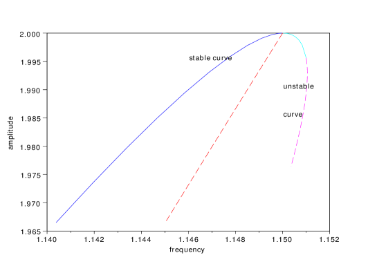
Figure 1: amplitude versus frequency of stationary forced solution in blue and magenta; amplitude of free solution in red

We have numerically solved equation (81) for a range of sigma around the value $\sigma=\frac{3da^{2}}{8\omega}$ for which the amplitude is maximum; we have chosen $\epsilon=.1;\lambda=1/2;F=1;\omega=1;d=1$; in figure 1, the solid line shows the solution of this equation that we have solved with several values of sigma using the routine fsolve of Scilab which implements a modification of the Powell hybrid method. We have noticed in proposition 2.2 that the solution is stable when $\sigma$ is not too large; indeed the routine fsolve fails to solve the equation when we increase too much $\sigma$; to go further this point, with the same routine, we have computed various values of sigma for decreasing values of the amplitude; we have plotted this solution with a magenta dotted line. We have added a red dotted line which is the amplitude of the free undamped solution and we notice that it crosses the stationary solution at the point where it reaches its maximum value as stated in previous proposition 2.2.

2.2.6 Dynamic solution

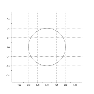
Figure 2: Phase portrait for $u_{0}=0.019796915,\omega_{\epsilon}=1.0143379$

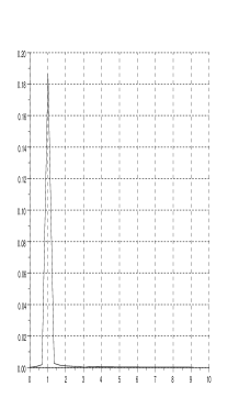
Figure 3: Absolute value of the Fourier transform for $u_{0}=0.019796915,\omega_{\epsilon}=1.0143379$

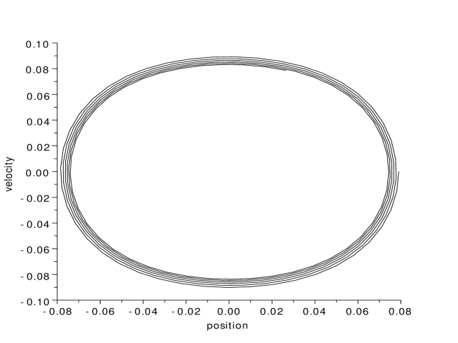
Figure 4: Phase portrait for $u_{0}=0.079,\omega_{\epsilon}=1.0143379$

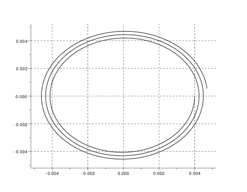
Figure 5: Phase portrait for $u_{0}=0.004,\omega_{\epsilon}=1.0143379$

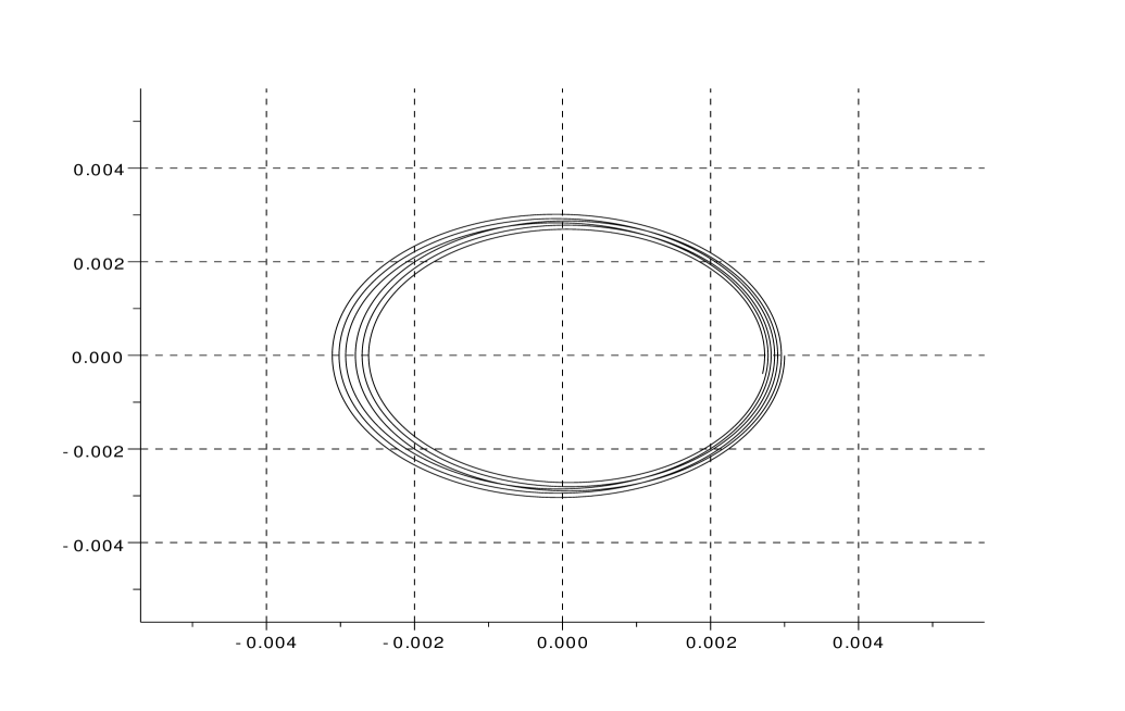
Figure 6: Phase portrait for $u_{0}=0.003,\omega_{\epsilon}=0.5$

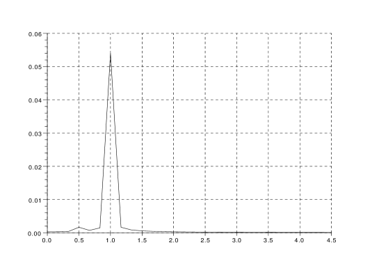
Figure 7: Fourier transform for $u_{0}=0.003,\omega_{\epsilon}=0.5$

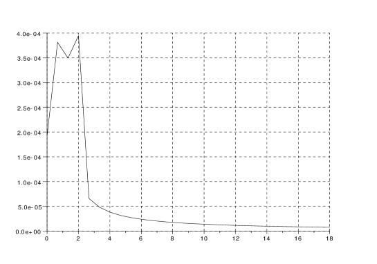
Figure 8: Fourier transform for $u_{0}=0.0001,\omega_{\epsilon}=2$

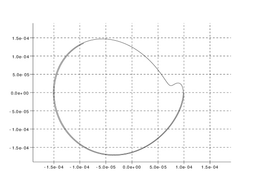
Figure 9: Phase portrait for $u_{0}=0.0001,\omega_{\epsilon}=2$

For various values of the initial condition, we compute numerically the solution of (26) with a standard theta method. We use $\epsilon=.01,\lambda=1/2,F=1;\omega=1,d=1$

In figure 3, we find the phase portrait of the solution with initial values $u(0)=0.019796915,u^{\prime}(0)=0$ so that the angular frequency of the applied force is $\tilde{\omega}_{\epsilon}=1.0143379$ , we notice that the solution looks periodic (up to the numerical approximation of the method); the initial value of the displacement is computed from a value of $a,\sigma$ of the stationary solution (81) which is computed in the previous paragraph. The Fourier transform in figure 3 shows only one peak at the angular frequency $1.0143379$ which is the angular frequency of the applied force.

In figure 4 , for the same value of the frequency of the applied force, we find the phase portrait of the solution with initial values $u(0)=0.079,u^{\prime}(0)=0$; the initial value is larger than the one of the stationary solution and we notice that the solution is decreasing as expected from the stability of the stationary solution.

We find an analogous behavior with an initial value smaller than the stationary solution; in figure 5, for the same value of the frequency of the applied force, we find the phase portrait of the solution with initial values $u(0)=0.004,u^{\prime}(0)=0$; here the solution is increasing as expected from the stability of the stationary solution.

In the case where $a,\omega_{\epsilon}$ are far from the stationary curve, we suspect that the frequency content of the response will involve the frequency of the applied force and some frequency due to the system; in figure 6, we find for $a=0.3,\omega_{\epsilon}=0.5$ the phase portrait of the solution, the frequency transform is in figure 8; on this plot of the Fourier transform, we notice two peaks icluding the angular frequency $\omega_{\epsilon}=0.5$ of the applied load.

For large values of $\omega_{\epsilon}$, the phase portrait is less regular see figure 9 for $a=0.01,\omega_{\epsilon}=2$ ; we find also two peaks for the Fourier transform in figure 8.

3 System with a strong local cubic non linearity

In the previous section, we have derived a double scale expansion of a solution of a one degree of freedom free vibrations system and damped vibrations with sinusoidal forcing with frequency close to free vibration frequency. Now, we extend the results to the case of multiple degrees of freedom.

3.1 Free vibrations, double scale expansion

We consider a system of vibrating masses attached to springs:

$$M\ddot{u}+Ku+\Phi(u,\epsilon)=0.$$ (83)

The mass matrix $M$ and the rigidity matrix $K$ are assumed to be symmetric and positive definite. See an example in section 3.2.5 We assume that the non linearity is local, all components are zero except for two components $p-1,\;p$ which correspond to the endpoints of some spring assumed to be non linear:

$$\Phi_{p-1}(u,\epsilon)=c(u_{p}-u_{p-1})^{2}+\frac{d}{\epsilon}(u_{p}-u_{p-1})^{3},\;\Phi_{p}=-\Phi_{p-1},~{}~{}p=2,\dots,n$$ (84)

If the non linear spring would have been the first or the last one, the expression of the function $\Phi$ would depend on the boundary condition; each case would be solved using the same method with slight changes in some formulas. In order to get an approximate solution, we are going to write it in the generalized eigenvector basis:

$$K\phi_{k}=\omega_{k}M\phi_{k},\text{ with }\phi_{k}^{T}M\phi_{l}=\delta_{kl},~{}~{}~{}k,l=1\dots,n.$$ (85)

So we perform the change of function

$$u=\sum_{k=1}^{n}y_{k}\phi_{k}$$ (86)

we obtain

$$\ddot{y}_{k}+\omega_{k}^{2}y_{k}+\phi_{k}^{T}\Phi(\sum_{i=1}^{n}y_{i}\phi_{i},\epsilon)=0,~{}~{}~{}k=1\dots,n.$$ (87)

As $\Phi$ has only 2 components which are not zero, it can be written

$$\ddot{y}_{k}+\omega_{k}^{2}y_{k}+\left(\phi_{k,p-1}-\phi_{k,p}\right)\Phi_{p-1}(\sum_{i=1}^{n}y_{i}\phi_{i},\epsilon)=0,~{}~{}~{}k=1\dots,n$$ (88)

or more precisely

$$\ddot{y}_{k}+\omega_{k}^{2}y_{k}+\left(\phi_{k,p-1}-\phi_{k,p}\right)\Bigg{[}c\left(\sum_{i=1}^{n}y_{i}(\phi_{i,p}-\phi_{i,p-1})\right)^{2}+\\ \frac{d}{\epsilon}\left(\sum_{i=1}^{n}y_{i}(\phi_{i,p}--\phi_{i,p-1})\right)^{3}\Bigg{]}=0,~{}~{}~{}k=1\dots,n.$$ (89)

As for the 1 d.o.f. case, we use a double scale expansion to compute an approximate small solution; more precisely, we look for a solution close to the normal mode of the associated linear system; we denote this mode by subscript $1$; obviously by permuting the coordinates, this subscript could be anyone (different of $p$, this case would give similar results with slightly different formulas); we set

$$T_{0}=\omega_{1}t,\quad T_{1}=\epsilon t$$ (90)

and we use the ansatz:

$$y_{k}=\epsilon y_{k}^{1}(T_{0},T_{1})+\epsilon^{2}r_{k}(T_{0},T_{1},\epsilon)$$ (91)

so that

$$\frac{d^{2}y_{k}}{dt^{2}}=\epsilon\omega_{1}^{2}D^{2}_{0}y_{k}^{1}+\epsilon^{2}[2\omega_{1}D_{0}D_{1}y_{k}^{1}+\omega_{1}^{2}D_{0}^{2}r_{k}]+\epsilon^{3}[D_{1}^{2}y_{k}^{1}+\mathcal{D}_{2}r_{k}]$$ (92)

with

$$\mathcal{D}_{2}r_{k}=\frac{1}{\epsilon}\left(\frac{d^{2}r_{k}}{dt^{2}}-\omega_{1}^{2}D_{0}^{2}r_{k}\right)=2\omega_{1}D_{0}D_{1}r_{k}+\epsilon D_{1}^{2}r_{k}.$$ (93)

We plug previous expansions into (89). By identifying the coefficients of the powers of $\epsilon$ in the expansion of (88), we get:

$$\Bigg{\{}\begin{array}[h]{rl}&\omega_{1}^{2}D_{0}^{2}y_{k}^{1}+\omega_{k}^{2}y_{k}^{1}=0,\ k=1\dots,n\\ &\omega_{1}^{2}D_{0}^{2}r_{k}+\omega_{k}^{2}r_{k}=S_{2,k},\ k=1\dots,n\quad\text{ with }\\ \end{array}$$ (96)

to simplify, the manipulations, we set

$$\delta_{p}\phi_{l}=(\phi_{l,p}-\phi_{l,p-1}),$$

so:

$$S_{2,k}=\frac{-\delta_{p}\phi_{k}}{\epsilon^{2}}\Phi_{p-1}\left(\sum_{i}(\epsilon y_{i}^{1}+\epsilon^{2}r_{i})\phi_{i},\epsilon\right)-2\omega_{1}D_{0}D_{1}y_{k}^{1}-\epsilon{\cal R}_{k}$$ (97)

with

$${\cal R}_{k}=\left(D_{1}^{2}y_{k}^{1}+{\cal D}_{2}r_{k}\right)$$ (98)

and

$$S_{2,k}=\frac{-\delta_{p}\phi_{k}}{\epsilon^{2}}\left[c\left(\sum_{i}(\epsilon y_{i}^{1}+\epsilon^{2}r_{i})\delta_{p}\phi_{i}\right)^{2}+\frac{d}{\epsilon}\left(\sum_{i}(\epsilon y_{i}^{1}+\epsilon^{2}r_{i})\delta_{p}\phi_{i}\right)^{3}\right]\\ -2\omega_{1}D_{0}D_{1}y_{k}^{1}-\epsilon{\cal R}_{k}.$$ (99)

The formula may be expanded

$$S_{2,k}=-\delta_{p}\phi_{k}\left[c\sum_{i,j}y_{i}^{1}y_{j}^{1}\delta_{p}\phi_{i}\delta_{p}\phi_{j}+d\sum_{i,j,l}y_{i}^{1}y_{j}^{1}y_{l}^{1}\delta_{p}\phi_{i}\delta_{p}\phi_{j}\delta_{p}\phi_{l}\right]\\ -2\omega_{1}D_{0}D_{1}y_{k}^{1}-\epsilon R_{k}\left(y^{1},r,\epsilon\right)$$ (100)

where

$$R_{k}(y^{1},r,\epsilon)={\cal R}_{k}\\ +\delta_{p}\phi_{k}\Bigg{[}\epsilon c\sum_{i,j}\left(2y_{i}^{1}r_{j}+\epsilon r_{i}r_{j}\right)\delta_{p}\phi_{i}\delta_{p}\phi_{j}+\\ \epsilon d\sum_{ijl}\left(3y_{i}^{1}y_{j}^{1}r_{l}+3\epsilon y_{i}^{1}r_{j}r_{l}+3\epsilon^{2}r_{i}r_{j}r_{l}\right)\delta_{p}\phi_{i}\delta_{p}\phi_{j}\delta_{p}\phi_{l}\Bigg{]}.$$ (101)

We set $\theta(T_{0},T_{1})=T_{0}+\beta(T_{1})$ and we note that $D_{0}\theta=1,\;D_{1}\theta=D_{1}\beta$; we solve the first set of equations (96), imposing $O(\epsilon)$ initial Cauchy data for $k\neq 1$; we get:

$$y_{1}^{1}=a(T_{1})cos(\theta),\;\text{ and }y_{k}^{1}=O(\epsilon),\;k=2\dots n$$ (102)

we put terms involving $y_{k}^{1},\;k\geq 2$ into $R_{k}$; so we obtain

$$S_{2,1}=-\delta_{p}\phi_{1}\left[c\left(y_{1}^{1}\delta_{p}\phi_{1}\right)^{2}+d\left(y_{1}^{1}\delta_{p}\phi_{1}\right)^{3}\right]\\ -2\omega_{1}D_{0}D_{1}y_{1}^{1}-\epsilon R_{1}(y^{1},r,\epsilon)\text{ and }$$ (103)

$$S_{2,k}=-\delta_{p}\phi_{k}\left[c\left(y_{1}^{1}\delta_{p}\phi_{1}\right)^{2}+d\left(y_{1}^{1}\delta_{p}\phi_{1}\right)^{3}\right]\\ -\epsilon R_{k}(y^{1},r,\epsilon)\text{ for }k\neq 1.$$ (104)

Using (102), we get:

$$S_{2,1}=-\delta_{p}\phi_{1}\Big{[}\frac{ca_{1}^{2}}{2}(1+cos(2\theta))\left(\delta_{p}\phi_{1}\right)^{2}+\\ \frac{da_{1}^{3}}{4}\left((cos(3\theta)+3cos(\theta))(\delta_{p}\phi_{1})^{3}\right)\Big{]}+\\ 2\omega_{1}(D_{1}a_{1}sin(\theta)+a_{1}D_{1}\beta_{1}cos(\theta))-\epsilon R_{1}(y^{1},r,\epsilon)\text{ and }$$ (105)

$$S_{2,k}=-\delta_{p}\phi_{k}\Big{[}\frac{ca_{1}^{2}}{2}(1+cos(2\theta))\left(\delta_{p}\phi_{1}\right)^{2}+\\ \frac{da_{1}^{3}}{4}\left((cos(3\theta)+3cos(\theta))(\delta_{p}\phi_{1})^{3}\right)\Big{]}+\\ -\epsilon R_{k}(y^{1},r,\epsilon)\text{ for }k\neq 1.$$ (106)

We gather the terms at angular frequency $1$ in $S_{2,1}$

$$S_{2,1}=-\delta_{p}\phi_{1}\Big{[}\frac{da_{1}^{3}}{4}3cos(\theta)(\delta_{p}\phi_{1})^{3}\Big{]}\\ +2\omega_{1}(D_{1}a_{1}sin(\theta)+a_{1}D_{1}\beta_{1}cos(\theta))+S_{2,1}^{\sharp}-\epsilon R(y^{1},r,\epsilon)$$ (107)

with

$$S_{2,1}^{\sharp}=-\delta_{p}\phi_{1}\left[\frac{ca_{1}^{2}}{2}(1+cos(2\theta))(\delta_{p}\phi_{1})^{2}+\frac{da_{1}^{3}}{4}cos(3\theta)(\delta_{p}\phi_{1})^{3}\right].$$ (108)

If we enforce

$$D_{1}a_{1}=0,~{}\text{ and }~{}2\omega_{1}a_{1}D_{1}\beta_{1}=(\delta_{p}\phi_{1})^{4}\frac{3da^{3}}{4}\text{ so that }\\ a_{1}=a_{1,0},\quad\beta_{1}=\beta_{1,0}T_{1}\text{ with }\beta_{1,0}=\frac{3da^{2}}{8\omega}(\delta_{p}\phi_{1})^{4}T_{1}$$ (109)

the right hand side

$$S_{2,1}=S_{2,1}^{\sharp}-\epsilon R_{1}(y^{1},r,\epsilon)$$ (110)

contains no term at angular frequency $1$; for the other components, without any manipulation, there is no trouble with the frequencies if we assume that all the eigenfrequencies $\omega_{k}$ for $k=2\dots n$ are not multiple of $\omega_{1}$ ($\omega_{k}\neq q\omega_{1}$ for $q=1$ or $q=2$, $q=3$).

In order to prove that $r$ is bounded, after the elimination of terms at frequency $1$, we write back the equations with the variable $t$, for the second set of equations of (96).

$$\omega_{1}^{2}\ddot{r}_{k}+\omega_{k}^{2}r_{k}=\tilde{S}_{2,k}\quad\text{ for }k=1,\dots n$$ (111)

with

$$\tilde{S}_{2,1}=S_{2,1}^{\sharp}-\epsilon\tilde{R}_{1}(y^{1},r,\epsilon)$$ (112)

where

$$S_{2,1}^{\sharp}=-\delta_{p}\phi_{1}\bigg{[}\frac{ca_{1}^{2}}{2}(1+cos(2(\omega_{1}t+\beta_{1,0}\epsilon t))(\delta_{p}\phi_{1})^{2}\\ +\frac{da_{1}^{3}}{4}cos(3(\omega_{1}t+\beta_{1,0}\epsilon t))(\delta_{p}\phi_{1})^{3}\bigg{]}$$ (113)

and

$$\tilde{S}_{2,k}=-\delta_{p}\phi_{k}\Bigg{[}\frac{ca_{1}^{2}}{2}(1+cos(2(\omega_{1}t+\beta_{1,0}\epsilon t)))\left(\delta_{p}\phi_{1}\right)^{2}+\\ \frac{da_{1}^{3}}{4}\left((cos(3(\omega_{1}t+\beta_{1,0}\epsilon t))+3cos((\omega_{1}t+\beta_{1,0}\epsilon t)))(\delta_{p}\phi_{1})^{3}\right)\Bigg{]}\\ -\epsilon\tilde{R}_{k}(y^{1},r,\epsilon)\text{ for }k\neq 1$$ (114)

and where

$$\tilde{R}_{k}(y^{1},r,\epsilon)=R_{k}(y^{1},r,\epsilon)-{\cal D}_{2}r_{k}$$ (115)

Proposition 3.1.

Under the assumption that $\omega_{k}$ and $\omega_{1}$ are $\mathbb{Z}$ independent for $k\neq 1$, there exists $\gamma>0$ such that for all $t\leq t_{\epsilon}=\frac{\gamma}{\epsilon}$, the solution of (88) with initial data

$$y_{1}(0)=\epsilon a_{1,0},\quad\dot{y}_{1}(0)=0,\quad y_{k}(0)=O(\epsilon^{2}),\quad\dot{y}_{k}(0)=0$$ (116)

satisfy the following expansion

$$y_{1}(t) =\epsilon a_{0}cos(\nu_{\epsilon}t)+\epsilon^{2}r_{1}(\epsilon,t)\text{ with }\nu_{\epsilon}=\omega_{1}+3\epsilon\frac{da_{0}^{2}}{8\omega_{1}}(\phi_{1,p}-\phi_{1,p-1})^{4}$$ (117)

$$y_{k}(t) =\epsilon^{2}r_{k}(\epsilon,t)$$ (118)

with $r_{k}$ uniformly bounded in ${\cal C}^{2}(0,t_{\epsilon})$ for $k=1,\dots n$ and $\omega_{1},\phi_{1}$ are the eigenvalue and eigenvectors defined in (85).

Corollary 3.1.

The solution of (83), (84) with

$$\phi_{1}^{T}u(0)=\epsilon a_{1,0},~{}~{}\phi_{1}^{T}\dot{u}(0)=0,~{}~{}\phi_{k}^{T}u(0)=O(\epsilon^{2}),~{}~{}\phi_{k}^{T}\dot{u}(0)=0$$

with $\omega_{k},\phi_{k}$ are the eigenvalue and eigenvectors defined in (85)

$$\text{ is }~{}~{}~{}u(t)=\sum_{k=1}^{n}y_{k}(t)\phi_{k}$$ (119)

with the expansion of $y_{k}$ of previous proposition.

Proof.

For the proposition, we use lemma 5.4. Set $S_{1}=S_{2,1}^{\sharp},~{}~{}S_{k}=S_{2,k}$ for $k=1,\dots n$; as we have enforced (109), the functions $S_{k}$ are periodic, bounded, and are orthogonal to $e^{\pm it}$, we have assumed that $\omega_{k}$ and $\omega_{1}$ are $\mathbb{Z}$ independent for $k\neq 1$; so $S_{k},~{}k=1,\dots,n$ satisfies the lemma hypothesis. Similarly, set $g=\tilde{R}$, its components are polynomials in $r$ with coefficients which are bounded functions, so it is lipschitzian on the bounded subsets of $\mathbb{R}$, it satisfies the hypothesis of lemma 5.4 and so the proposition is proved. The corollary is an easy consequence of the proposition and the change of function (121) ∎

Remark 3.1.

We have obtained a periodic asymptotic expansion of a solution of system (83), (84); they are called non linear normal modes in the mechanical community ([KPGV09, JPS04]. In the next section, we shall derive that the frequencies of the normal mode are resonant frequencies for an associated forced system, the so called primary resonance; secondary resonance could be derived along similar lines.

3.2 Forced, damped vibrations, double scale expansion

3.2.1 Derivation of the expansion

We consider a similar system of forced vibrating masses attached to springs with a light damping:

$$M\ddot{u}+\epsilon C\dot{u}+Ku+\Phi(u,\epsilon)=\epsilon^{2}Fcos(\tilde{\omega}_{\epsilon}t)$$ (120)

with the same assumptions as in subsection 3.1. We assume that the frequency of the driving force is close to some frequency of the linearised system (primary resonance); we denote this frequency with the subscript $1$: $\tilde{\omega}_{\epsilon}=\omega_{1}+\epsilon\sigma.$

We assume that the non linearity is local, all components are zero except for two components $p-1,\;p$ which correspond to the endpoints of some spring assumed to be non linear. As for free vibrations, we perform the change of function

$$u=\sum_{k=1}^{n}y_{k}\phi_{k}$$ (121)

with $\phi_{k}$, the generalised eigenvectors of (85). As the damping matrix $C$ is usually not well defined, to simplify, we assume that it is diagonal in the eigenvector basis $\phi_{k},\;k=1,\dots n$. We obtain

$$\ddot{y}_{k}+\epsilon\lambda_{k}\dot{y}_{k}+\omega_{k}^{2}y_{k}+\phi_{k}^{T}\Phi(\sum_{i=1}^{n}y_{i}\phi_{i},\epsilon)=\epsilon^{2}f_{k}cos(\tilde{\omega}_{\epsilon}t),~{}~{}~{}k=1\dots,n$$ (122)

with $f_{k}=\phi_{k}^{T}F$. As for the free vibration case, $\Phi$ has only 2 components which are not zero, so the system can be written

$$\ddot{y}_{k}+\epsilon\lambda_{k}\dot{y}_{k}+\omega_{k}^{2}y_{k}+\left(\phi_{k,p-1}-\phi_{k,p},\epsilon\right)\Phi_{p-1}(\sum_{i=1}^{n}y_{i}\phi_{i})=\epsilon^{2}f_{k}cos(\tilde{\omega}_{\epsilon}t),\\ ~{}~{}~{}k=1\dots,n$$ (123)

or more precisely

$$\ddot{y}_{k}+\epsilon\lambda_{k}\dot{y}_{k}+\omega_{k}^{2}y_{k}+\left(\phi_{k,p-1}-\phi_{k,p}\right)\Bigg{[}c\left(\sum_{i=1}^{n}y_{i}(\phi_{i,p}-\phi_{i,p-1})\right)^{2}+\\ \frac{d}{\epsilon}\left(\sum_{i=1}^{n}y_{i}(\phi_{i,p}-\phi_{i,p-1})\right)^{3}\Bigg{]}=\epsilon^{2}f_{k}cos(\tilde{\omega}_{\epsilon}t),\\ ~{}~{}~{}k=1\dots,n.$$ (124)

As for the 1 d.o.f. case, we use a double scale expansion to compute an approximate small solution; we use a fast scale which is $\epsilon$ dependent; we set

$$T_{0}=\tilde{\omega}_{\epsilon}t,\quad T_{1}=\epsilon t$$ (125)

and we use the “ansatz”

$$y_{k}=\epsilon y_{k}^{1}(T_{0},T_{1})+\epsilon^{2}r_{k}(T_{0},T_{1},\epsilon)$$ (126)

so that

$$\frac{dy_{k}}{dt}=\epsilon\big{[}\omega_{1}D_{0}y_{k}^{1}+\epsilon\sigma D_{0}y_{k}^{1}+\epsilon D_{1}y_{k}^{1}\big{]}+\epsilon^{2}\omega_{1}D_{0}r_{k}+\epsilon^{2}(\frac{dr_{k}}{dt}-\omega_{1}D_{0}r_{k})$$ (127)

$$\frac{d^{2}y_{k}}{dt^{2}}=\epsilon\bigg{\{}\omega_{1}^{2}D_{0}^{2}y_{k}^{1}+2\epsilon\omega_{1}\left[\sigma D_{0}^{2}y_{k}^{1}+D_{0}D_{1}y_{k}^{1}\right]+\\ \epsilon^{2}\left[\sigma^{2}D_{0}^{2}y_{k}^{1}+2\sigma D_{0}D_{1}y_{k}^{1}+D_{1}^{2}y_{k}^{1}\right]\bigg{\}}\\ +\epsilon^{2}\omega_{1}^{2}D_{0}^{2}r_{k}+\epsilon^{3}\mathcal{D}_{2}r_{k}$$ (128)

with

$$\mathcal{D}_{2}r_{k}=\frac{1}{\epsilon}\left(\frac{d^{2}r_{k}}{dt^{2}}-\omega_{1}^{2}D_{0}^{2}r_{k}\right)=2\omega_{1}(\sigma D_{0}^{2}r_{k}+D_{0}D_{1}r_{k})\\ +\epsilon\left[\sigma^{2}D_{0}^{2}r_{k}+2\sigma D_{0}D_{1}r_{k}+D_{1}^{2}r_{k}\right].$$ (129)

We plug previous expansions into (124). By identifying the coefficients of the powers of $\epsilon$ in the expansion of (124), we get:

$$\Bigg{\{}\begin{array}[h]{rl}&\omega_{1}^{2}D_{0}^{2}y_{k}^{1}+\omega_{k}^{2}y_{k}^{1}=0,\ k=1\dots,n\\ &\omega_{1}^{2}D_{0}^{2}r_{k}+\omega_{k}^{2}r_{k}=S_{2,k},\ k=1\dots,n\quad\text{ with }\\ \end{array}$$ (132)

$$S_{2,k}=-\Bigg{\{}\frac{\delta_{p}\phi_{k}}{\epsilon^{2}}\Phi_{p-1}\left(\sum_{i}(\epsilon y_{i}^{1}+\epsilon^{2}r_{i})\phi_{i},\epsilon\right)+2\omega_{1}[D_{0}D_{1}y_{k}^{1}+\sigma D_{0}^{2}y_{k}^{1}]+\lambda_{k}\omega_{1}D_{0}y_{k}^{1}\Bigg{\}}\\ +f_{k}cos(T_{0})-\epsilon R_{k}(y^{1},r,\epsilon)$$ (133)

where we gather higher order terms in $R_{k}$ and to simplify, the manipulations, we have set

$$\delta_{p}\phi_{l}=(\phi_{l,p}-\phi_{l,p-1}),$$

so:

$$S_{2,k}=-\frac{\delta_{p}\phi_{k}}{\epsilon^{2}}\left[c\left(\sum_{i}(\epsilon y_{i}^{1}+\epsilon^{2}r_{i})\delta_{p}\phi_{i}\right)^{2}+\frac{d}{\epsilon}\left(\sum_{i}(\epsilon y_{i}^{1}+\epsilon^{2}r_{i})\delta_{p}\phi_{i}\right)^{3}\right]\\ -2\omega_{1}[D_{0}D_{1}y_{k}^{1}+\sigma D_{0}^{2}y_{k}^{1}]-\lambda_{k}\omega_{1}D_{0}y_{k}^{1}\\ +f_{k}cos(T_{0})-\epsilon R_{k}(y^{1},r,\epsilon).$$ (134)

The formula may be expanded

$$S_{2,k}=-\delta_{p}\phi_{k}\left[c\sum_{i,j}y_{i}^{1}y_{j}^{1}\delta_{p}\phi_{i}\delta_{p}\phi_{j}+d\sum_{i,j,l}y_{i}^{1}y_{j}^{1}y_{l}^{1}\delta_{p}\phi_{i}\delta_{p}\phi_{j}\delta_{p}\phi_{l}\right]\\ -2\omega_{1}[D_{0}D_{1}y_{k}^{1}+\sigma D_{0}^{2}y_{k}^{1}]-\lambda_{k}\omega_{1}D_{0}y_{k}^{1}\\ +f_{k}cos(T_{0})-\epsilon R_{k}(y^{1},r,\epsilon)$$ (135)

We set $\theta(T_{0},T_{1})=T_{0}+\beta(T_{1})$ and we note that $D_{0}\theta=1,\;D_{1}\theta=D_{1}\beta$; we solve the first set of equations (132), imposing initial Cauchy data for $k\neq 1$ of order $O(\epsilon)$ we get:

$$y_{1}^{1}=a_{1}(T_{1})cos(\theta),\;\text{ and }y_{k}^{1}=O(\epsilon),\;k=2\dots n$$ (136)

we put terms involving $y_{k}^{1}$ into $R_{k}$ for $k\geq 2$ and so we obtain

$$S_{2,1}=-\delta_{p}\phi_{1}\left[c\left(y_{1}^{1}\delta_{p}\phi_{1}\right)^{2}+d\left(y_{1}^{1}\delta_{p}\phi_{1}\right)^{3}\right]\\ -2\omega_{1}[D_{0}D_{1}y_{1}^{1}+\sigma D_{0}^{2}y_{1}^{1}]-\lambda_{1}\omega_{1}D_{0}y_{1}^{1}+f_{1}\cos(T_{0})-\epsilon R_{1}(y^{1},r,\epsilon)\text{ and }$$ (137)

$$S_{2,k}=-\delta_{p}\phi_{k}\left[c\left(y_{1}^{1}\delta_{p}\phi_{1}\right)^{2}+d\left(y_{1}^{1}\delta_{p}\phi_{1}\right)^{3}\right]+\\ f_{k}\cos(T_{0})-\epsilon R_{k}(y^{1},r,\epsilon)\text{ for }k\neq 1.$$ (138)

Using (136), we get:

$$S_{2,1}=-\delta_{p}\phi_{1}\Big{[}\frac{ca_{1}^{2}}{2}(1+\cos(2\theta))\left(\delta_{p}\phi_{1}\right)^{2}+\\ \frac{da_{1}^{3}}{4}\left((\cos(3\theta)+3\cos(\theta))(\delta_{p}\phi_{1})^{3}\right)\Big{]}+\\ 2\omega_{1}[D_{1}a_{1}sin(\theta)+a_{1}D_{1}\beta_{1}\cos(\theta)+\sigma a_{1}\cos(\theta)]+\lambda_{1}\omega_{1}a_{1}sin(\theta)\\ +f_{1}[\sin(\theta)\sin(\beta)+\cos(\theta)\cos(\beta)]-\epsilon R_{1}(y^{1},r,\epsilon)\text{ and }$$ (139)

$$S_{2,k}=-\delta_{p}\phi_{k}\Big{[}\frac{ca_{1}^{2}}{2}(1+\cos(2\theta))\left(\delta_{p}\phi_{1}\right)^{2}+\\ \frac{da_{1}^{3}}{4}\left((\cos(3\theta)+3\cos(\theta))(\delta_{p}\phi_{1})^{3}\right)\Big{]}+\\ +f_{k}[\sin(\theta)\sin(\beta)+\cos(\theta)\cos(\beta)]-\epsilon R_{k}(y^{1},r,\epsilon)\text{ for }k\neq 1.$$ (140)

We gather the terms at angular frequency $1$ in $S_{2,1}$

$$S_{2,1}=\delta_{p}\phi_{1}\Bigg{[}-3\frac{da_{1}^{3}}{4}\cos(\theta)(\delta_{p}\phi_{1})^{3}+2\omega_{1}(a_{1}D_{1}\beta_{1}+\sigma a_{1})+f_{1}\cos(\beta)\Bigg{]}\cos(\theta)\\ +\Big{[}\omega_{1}(2D_{1}a_{1}+\lambda_{1}a_{1})+f_{1}sin(\beta)\Big{]}sin(\theta)+S_{2,1}^{\sharp}-\epsilon R(y^{1},r,\epsilon)$$ (141)

with

$$S_{2,1}^{\sharp}=-\delta_{p}\phi_{1}\left[\frac{ca_{1}^{2}}{2}(1+\cos(2\theta))(\delta_{p}\phi_{1})^{2}+\frac{da_{1}^{3}}{4}\cos(3\theta)(\delta_{p}\phi_{1})^{3}\right].$$ (142)

Orientation

If we enforce

$$\Bigg{\{}\begin{array}[h]{rl}\omega_{1}\big{(}2D_{1}a_{1}+\lambda_{1}a_{1}\big{)}&=-f_{1}sin(\beta_{1}),~{}~{}\text{ and }\\ ~{}2\omega_{1}\big{(}a_{1}D_{1}\beta_{1}+\sigma a_{1}\big{)}&=\frac{3da^{3}}{4}(\delta_{p}\phi_{1})^{4}-f_{1}cos(\beta_{1})\end{array}$$ (143)

the right hand side

$$S_{2,1}=S_{2,1}^{\sharp}-\epsilon R_{1}(y^{1},r,\epsilon)$$ (144)

contains no term at angular frequency $1$; for the other components, without any manipulation, there is not such terms , if we assume that all the eigenfrequencies $\omega_{k}$ for $k=2\dots n$ are not multiple of $\omega_{1}$ ($\omega_{k}\neq q\omega_{1}$ for $q=1$ or $q=2$, $q=3$). This will enable us to justify this expansion; previously, we study the stationary solution of this approximate system and the stability of the solution in a neighbourhood of this stationary solution.

3.2.2 Stationary solution and stability

The situation is very close to the 1 d.o.f. case; except the replacement of $d$ by of $\tilde{d}=d(\delta_{p}\phi_{1})^{4}$, the system (143) is the same as (57); the other components are zero. We state a similar proposition

Proposition 3.2.

When $\sigma\leq\frac{3\tilde{d}\bar{a}^{2}}{4\omega}-\frac{1}{2}\sqrt{\frac{9\tilde{d}^{2}\bar{a}^{4}}{16\omega^{2}}-\lambda_{1}^{2}}$ , the stationary solution of (143) is stable in the sense of Lyapunov (if the dynamic solution starts close to the stationary one, it remains close and converges to it); to the stationary case corresponds the approximate solution of (89) $y_{1}^{1}=\bar{a}_{1}\cos(T_{0}+\bar{\beta}_{1}),~{}~{}y_{k}^{1}=O(\epsilon),~{}~{}k=2,\dots,n$, it is periodic; for an initial data close enough to the stationary solution, $y_{1}^{1}=a(T_{1})\cos(T_{0}+\beta_{1}(T_{1})),~{}~{}y_{k}^{1}=O(\epsilon),~{}~{}k=2,\dots,n$ with $a,\beta_{1}$ solutions of (143) with $d$ replaced by $\tilde{d}$ ; they converge to the stationary solution $\bar{a}_{1},\bar{\beta}_{1}$ when $T_{1}\longrightarrow+\infty$.

3.2.3 Convergence of the expansion

In order to prove that $r$ is bounded, after the elimination of terms at frequency $1$, we write back the equations with the variable $t$, for the second set of equations of (96).

$$\omega_{1}^{2}\ddot{r}_{k}+\omega_{k}^{2}r_{k}=\tilde{S}_{2,k}\quad\text{ for }k=1,\dots n$$ (145)

with

$$\tilde{S}_{2,1}=S_{2,1}^{\sharp}-\epsilon\tilde{R}_{1}(y^{1},r,\epsilon)$$ (146)

where

$$S_{2,1}^{\sharp}=-\delta_{p}\phi_{1}\bigg{[}\frac{c(a_{1}(\epsilon t))^{2}}{2}(1+\cos(2(\tilde{\omega}_{\epsilon}t+\beta_{1}(\epsilon t))(\delta_{p}\phi_{1})^{2}\\ +\frac{da_{1}^{3}}{4}\cos(3(\tilde{\omega}_{\epsilon}t+\beta_{1}(\epsilon t))(\delta_{p}\phi_{1})^{3}\bigg{]}$$ (147)

and

$$S_{2,k}=-\delta_{p}\phi_{k}\Bigg{[}\frac{c(a_{1}(\epsilon t)^{2}}{2}(1+\cos(2(\tilde{\omega}_{\epsilon}t+\beta_{1}(\epsilon t)))\left(\delta_{p}\phi_{1}\right)^{2}+\\ \frac{da_{1}^{3}}{4}\left((\cos(3(\tilde{\omega}_{\epsilon}t+\beta_{(}\epsilon t))+3\cos((\tilde{\omega}_{\epsilon}t+\beta_{1}(\epsilon t)))(\delta_{p}\phi_{1})^{3}\right)\Bigg{]}\\ -\epsilon R_{k}(y^{1},r,\epsilon)\text{ for }k\neq 1$$ (148)

where

$$\tilde{R}_{k}(y^{1},r,\epsilon)=R_{k}(y^{1},r,\epsilon)-{\cal D}_{2}r_{k}-\lambda_{k}\bigl{(}\frac{dr_{k}}{dt}-\omega_{k}D_{0}r_{k}\bigr{)}$$ (149)

Proposition 3.3.

Under the assumption that $\omega_{k}$ and $\omega_{1}$ are $\mathbb{Z}$ independent for $k\neq 1$, there exists $\gamma>0$ such that for all $t\leq t_{\epsilon}=\frac{\gamma}{\epsilon}$, the solution of (124) with initial data

$$y_{1}(0)=\epsilon a_{1,0}+O(\epsilon^{2}),\quad\dot{y}_{1}(0)=-\epsilon\omega a_{1,0}sin(\beta_{1,0})+O(\epsilon^{2}),$$ (150)

$$\quad y_{k}(0)=O(\epsilon^{2}),\quad\dot{y}_{k}(0)=0$$ (151)

and with the initial data close to the stationary solution

$$|a_{1,0}-\bar{a}_{1}|\leq\epsilon C_{1},~{}~{}|\beta_{1,0}-\bar{\beta}_{1}|\leq\epsilon C_{1}$$

satisfy the following expansion

$$y_{1}(t) =\epsilon a_{1}(\epsilon t)\cos(\tilde{\omega}_{\epsilon}t+\beta_{1}(\epsilon t))+\epsilon^{2}r_{1}(\epsilon,t)\text{ with }$$ (152)

$$y_{k}(t) =\epsilon^{2}r_{k}(\epsilon,t)$$ (153)

with $a_{1},\beta_{1}$ solution of (143) and with $r_{k}$ uniformly bounded in ${\cal C}^{2}(0,t_{\epsilon})$ for $k=1,\dots n$ and $\omega_{1},\phi_{1}$ are the eigenvalue and eigenvectors defined in (85) and $a_{1}\beta_{1}$ are solution of (143)

Corollary 3.2.

The solution of (120), (84) with

$$\phi_{1}^{T}u(0)=\epsilon a_{1,0},~{}~{}\phi_{1}^{T}\dot{u}(0)=-\epsilon\omega_{1}a_{1,0}\sin(\beta_{1,0}),~{}~{}\phi_{k}^{T}u(0)=O(\epsilon^{2}),~{}~{}\phi_{k}^{T}\dot{u}(0)=0$$

with $\omega_{k},\phi_{k}$ the eigenvalues and eigenvectors defined in (85).

$$\text{ is }~{}~{}~{}u(t)=\sum_{k=1}^{n}y_{k}(t)\phi_{k}$$ (154)

with the expansion of $y_{k}$ of previous proposition.

Proof.

For the proposition, we use lemma 5.4. Set $S_{1}=S_{2,1}^{\sharp},~{}~{}S_{k}=S_{2,k}$ for $k=1,\dots n$; as we have enforced (109), the functions $S_{k}$ are periodic, bounded, and are orthogonal to $e^{\pm it}$, we have assumed that $\omega_{k}$ and $\omega_{1}$ are $\mathbb{Z}$ independent for $k\neq 1$; so $S$ satisfies the lemma hypothesis. Similarly, set $g=\tilde{R}$, it is a polynomial in $r$ with coefficients which are bounded functions , so it is lipschitzian on the bounded subsets of $\mathbb{R}$, it satisfies the hypothesis of lemma 5.4 and so the proposition is proved. The corollary is an easy consequence of the proposition and the change of function (121) ∎

3.2.4 Maximum of the stationary solution

As equation (143) is similar to the equation (57) of the 1 d.o.f. case, we get also that the stationary solution reaches its maximum amplitude to the frequency of the free periodic solution.

Consider the stationary solution of (143), it satisfies

$$\Bigg{\{}\begin{array}[h]{rl}\lambda_{1}a_{1}\omega_{1}&=-f_{1}\sin(\beta_{1})\\ a\left(2\omega_{1}\sigma-\frac{3\tilde{d}a^{2}}{4}\right)&=-f_{1}\cos(\beta_{1})\end{array}$$ (157)

manipulating, we get that $a_{1}$ is solution of the equation:

$$f(a_{1},\sigma)=\lambda_{1}^{2}a_{1}^{2}\omega^{2}+a_{1}^{2}\left(2\omega_{1}\sigma-\frac{3\tilde{d}a_{1}^{2}}{4}\right)^{2}-f_{1}^{2}=0.$$ (158)

As for the 1 d.o.f. case, we can state:

Proposition 3.4.

The stationary solution of (143) satisfies

$$\Bigg{\{}\begin{array}[h]{rl}\lambda_{1}a_{1}\omega_{1}&+f_{1}\sin(\beta_{1})=0\\ 2a_{1}\omega_{1}\sigma-\frac{3\tilde{d}a^{3}}{4}&+f_{1}\cos(\beta_{1})=0\end{array}$$ (161)

it reaches its maximum amplitude for $\sigma=\frac{3\tilde{d}a_{1}^{2}}{8\omega_{1}}$ and $\beta_{1}=\frac{\pi}{2}+k\pi$; the excitation is at the frequency

$$\tilde{\omega}_{\epsilon}=\omega_{1}+3\epsilon\frac{\tilde{d}a_{1}^{2}}{8\omega_{1}},~{}\text{ with }~{}\tilde{d}=d(\Phi_{1,p}-\Phi_{1,p-1})^{4}~{}~{}\text{ and }~{}F=\lambda_{1}\omega_{1}a_{1}$$

where $\Phi_{1}$ is the eigenvector of the underlying linear system associated to $\omega_{1}$; $\tilde{\omega}_{\epsilon}$ is the frequency of the free periodic solution (25); for this frequency, the approximation (of the solution up to the order $\epsilon$) is periodic:

$$y_{1}(t) =\epsilon\frac{f_{1}}{\lambda_{1}\omega_{1}}\sin(\tilde{\omega}_{\epsilon}t)+\epsilon^{2}r(\epsilon,t)$$ (162)

$$y_{k}(t) =\epsilon^{2}r_{k}(\epsilon,t)$$ (163)

As for the 1 d.o.f. case we can remark the following points.

Remark 3.2.

This value of $\sigma=\frac{3\tilde{d}a_{1}^{2}}{8\omega_{1}}$ is indeed smaller than the maximal value that $\sigma$ may reach in order that the system be stable and that the previous expansion converges as indicated in proposition 2.3.

Remark 3.3.

We note also that when the stationary solution reaches its maximum amplitude we have $f_{1}=\lambda_{1}\omega_{1}a_{1}$ and so we can recover the damping ratio $\lambda_{1}$ from such a forced vibration experiment; this is a close link with the linear case (see for example [GR93] or the English translation [GR97]). This is quite interesting in practice as the damping ratio is usually difficult to measure. Obviously, we can recover the damping ratio for other frequencies by performing other experiments.

We can also consider this result as a stability of the process used in the linear case with respect to the appearance of a small non-linearity.

3.2.5 Numerical solution

We consider numerical solution of (120) with (84); we have chosen $M=I$; $u=0$ at both ends, so $K$ is the classical matrix

$$k\begin{pmatrix}2&-1&[]{3}\\ -1&2&-1&{2}\\ 0&-1&2&-1&\dots\\ []{5}\\ []{3}&-1&2\end{pmatrix};$$

$C=\lambda I$ with $\lambda=1/2$; for numerical balance, we have computed $\frac{u}{\epsilon}$; with the choice $p=1$ we have $\Phi_{1}=\epsilon[cu_{1}^{2}+du_{1}^{3}]$ with $c=1,d=1$. In figure 10, we find 3 curves in phase space for components $1,3,6$ of the system. In figure 11, we find the Fourier transform of the components; some components have the same transform; the graphs are slightly non symmetric.

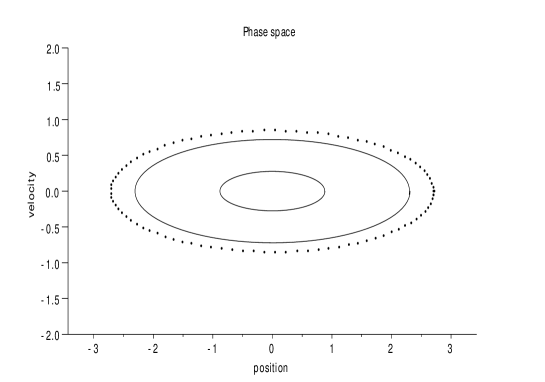
Figure 10: Phase portrait of a system with 9 d.o.f. for $\omega_{\epsilon}=0.3128868$

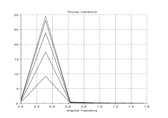
Figure 11: Phase portrait of a system with 9 d.o.f. for $\omega_{\epsilon}=0.3128868$

4 Conclusion

For differential systems modeling spring-masses vibrations with non linear springs, we have derived and rigorously proved a double scale analysis of periodic solution of free vibrations (so called non linear normal modes); for damped vibrations with periodic forcing with frequency close to free vibration frequency ( the so called primary resonance case), we have obtained an asymptotic expansion and derived that the amplitude is maximal at the frequency of the non linear normal mode. Such non linear vibrating systems linked to a bar generate acoustic waves; an analysis of the dilatation of a one-dimensional nonlinear crack impacted by a periodic elastic wave, a smooth model of the crack may be carried over with a delay differential equation, [jl09].

Acknowledgment

We thank S. Junca for his stimulating interest.

5 Appendix

5.1 Inequalities for differential equations

Lemma 5.1.

Let $w_{\epsilon}$ be solution of

$$w"+w=S(t,\epsilon)+\epsilon g(t,w,\epsilon)$$ (164)

$$w(0)=0,\quad w^{\prime}(0)=0.$$ (165)

If the right hand side satisfies the following conditions

1. $S$ is a sum of periodic bounded functions:

   1. for all $t$ and for all $\epsilon$ small enough, $S(t,\epsilon)\leq M$

   2. $\int_{0}^{2\pi}e^{it}S(t,\epsilon)dt=0,\quad\int_{0}^{2\pi}e^{-it}S(t,\epsilon)dt=0$ uniformly for $\epsilon$ small enough

2. for all $R>0$, there exists $k_{R}$ such that for $|u|\leq R$ and $|v|\leq R$, the inequality $|g(t,u,\epsilon)-g(t,v,\epsilon)|\leq k_{R}|u-v|$ holds and $|g(t,0,\epsilon)|$is bounded; in other words $g$ is locally lipschitzian with respect to u.

then, there exists $\gamma>0$ such that for $\epsilon$ small enough, $w_{\epsilon}$ is uniformly bounded in $C^{2}(0,T_{\epsilon})$ with $T_{\epsilon}=\frac{\gamma}{\epsilon}$

Proof.

The proof is close to the proof of lemma 6.3 of [JR10]; but it is technically simpler since here we assume $g$ to be locally lipschitzian with respect to $u$ whereas it is only bounded in [JR10].

1. We first consider

   $$w_{1}"+w_{1}=S(t,\epsilon)$$ (166)

   $$w_{1}(0)=0,\quad w_{1}^{\prime}(0)=0$$ (167)

   as $S$ is a sum of periodic functions which are uniformly orthogonal to $e^{it}$ and $e^{-it}$, $w_{1}$ is bounded in ${\cal C}^{2}(0,+\infty).$

2. Then we perform a change of function: $w=w_{1}+w_{2}$, the following equalities hold

   $$w_{2}"+w_{2}=\epsilon g_{2}(t,w_{2},\epsilon)$$ (168)

   $$w_{2}(0)=0,\quad w_{2}^{\prime}(0)=0$$ (169)

   with $g_{2}$ which satisfies the same hypothesis as $g$:

   for all $R>0$, there exists $k_{R}$ such that for $|u|\leq R$ and $|v|\leq R$, the following inequality holds $|g_{2}(t,u,\epsilon)-g_{2}(t,v,\epsilon)|\leq k_{R}|u-v|$. Using Duhamel principle, the solution of this equation satisfies:

   $$w_{2}=\epsilon\int_{0}^{t}\sin(t-s)g_{2}(s,w_{2}(s),\epsilon)ds$$ (170)

   from which

   $$|w_{2}(t)|\leq\epsilon\int_{0}^{t}|g_{2}(s,w_{2}(s),\epsilon)-g_{2}(s,0,\epsilon)|ds+\epsilon\int_{0}^{t}|g_{2}(s,0,\epsilon)|ds$$ (171)

   so if $|w|\leq R$, hypothesis of lemma imply

   $$|w_{2}(t)|\leq\epsilon\int_{0}^{t}k_{R}|w_{2}|ds+\epsilon Ct.$$ (172)

   A corollary of lemma of Bellman-Gronwall, see below, will enable to conclude. It yields

   $$|w_{2}(t)|\leq\frac{C}{k_{R}}\left(\exp(\epsilon k_{R}t)-1\right).$$ (173)

   Now set $T_{\epsilon}=\sup\{t||w|\leq R\}$, then we have

   $$R\leq\frac{C}{k_{R}}\left(\exp(\epsilon k_{R}t)-1\right)$$

   this shows that there exists $\gamma$ such that $|w_{2}|\leq R$ for $t\leq T_{\epsilon}$, which means that it is in $L^{\infty}(0,T_{\epsilon})$ for $T_{\epsilon}=\frac{\gamma}{\epsilon}$; also, we have $w$ in ${\cal C}(0,T_{\epsilon})$ then as $w$ is solution of (164), it is also bounded in ${\cal C}^{2}(0,T_{\epsilon})$.

∎

Lemma 5.2.

(Bellman-Gronwall, [bel, Bel64]) Let $u,\epsilon,\beta$ be continuous functions with $\beta\geq 0$,

$$u(t)\leq\epsilon(t)+\int_{0}^{t}\beta(s)u(s)ds\text{ for }0\leq t\leq T$$ (174)

then

$$u(t)\leq\epsilon(t)+\int_{0}^{t}\beta(s)\epsilon(s)\left[\exp(\int_{s}^{t}\beta(\tau)d\tau\right]ds$$ (175)

Lemma 5.3.

( a consequence of previous lemma, suited for expansions, see [SV85]) Let $u$ be a positive function, $\delta_{2}\geq 0$, $\delta_{1}>0$ and

$$u(t)\leq\delta_{2}t+\delta_{1}\int_{0}^{t}u(s)ds$$

then

$$u(t)\leq\frac{\delta_{2}}{\delta_{1}}\left(exp(\delta_{1}t)-1\right)$$

Lemma 5.4.

Let $v_{\epsilon}=[v_{1}^{\epsilon},\dots,v_{N}^{\epsilon}]^{T}$ be the solution of the following system:

$$\omega_{1}^{2}(v_{k}^{\epsilon})"+\omega_{k}^{2}v_{k}^{\epsilon}=S_{k}(t)+\epsilon g_{k}(t,v_{\epsilon}).$$ (176)

If $\omega_{1}$ and $\omega_{k}$ are $\mathbb{Z}$ independent for all $k=2\dots N$ and the right hand side satisfies the following conditions with $M>0,\;C>0$ prescribed constants:

1. $S_{k}$ is a sum of bounded periodic functions, $|S_{k}(t)|\leq M$ which satisfy the non resonance conditions:

2. $S_{1}$ is orthogonal to $e^{\pm it}$, i.e. $\int_{0}^{2\pi}S_{1}(t)e^{\pm it}dt=0$ uniformly for $\epsilon$ going to zero

3. for all $R>0$ there exists $k_{R}$ such that for $\|u\|\leq R$, $\|v\|\leq R$, the following inequality holds for $k=1,\dots,N$ :

   $$|g_{k}(t,u,\epsilon)-g_{k}(t,v,\epsilon)|\leq k_{R}\|u-v\|$$

   and $|g_{k}(t,0,\epsilon)|$ is bounded

then there exists $\gamma>0$ such that for $\epsilon$ small enough $v_{\epsilon}$ is bounded in ${\cal C}^{2}(0,T_{\epsilon})$ with $T_{\epsilon}=\frac{\gamma}{\epsilon}$

Proof.

1. We first consider the linear system

   $$\omega_{1}^{2}(v_{k,1})"+\omega_{k}^{2}v_{k,1}=S_{k}$$ (177)

   $$v_{k,1}(0)=0\text{ and }(v_{k,1})^{\prime}=0$$ (178)

   For $k=1$, with hypothesis 1.a, $S_{1}$ is a sum of bounded periodic functions; it is orthogonal to $e^{\pm it}$, there is no resonance. For $k\neq 1$, there is no resonance as $\frac{\omega_{k}}{\omega_{1}}\notin\mathbb{Z}$ with hypothesis 1.b.

   So $v_{k,1}$ belongs to $C^{(2)}$ for $k=1,...,n.$

2. Then we perform a change of function

   $$v_{k}^{\epsilon}=v_{k,1}+v_{k,2}^{\epsilon}$$

   and $v_{k,2}^{\epsilon}$ are solutions of the following system :

   $$\omega_{1}^{2}(v_{k,2})"+\omega_{k}^{2}v_{k,2}=\epsilon g_{k,2}(t,v_{k,2},\epsilon),~{}k=1,\dots,N$$ (179)

   $$v_{k,2}^{\epsilon}(0)=0,~{}(v_{k,2}^{\epsilon})^{\prime}=0,~{}k=1,\dots,N$$ (180)

   with

   $$g_{k,2}(t,....,v_{k,2}^{\epsilon},....)=g_{k}(t,...,v_{k,1}+v_{k,2}^{\epsilon},....)$$

   where $~{}g_{k,2}~{}$ satisfies the same hypothesis as $g_{k}$:
   for all $R>0$ there exists $k_{R}$ such that for $\parallel u_{k}\parallel\leq R$, $\parallel v_{k}\parallel\leq R$, the following inequality holds for $k=1,\dots,N$ :

   $$\parallel g_{k,2}(t,u_{k},\epsilon)-g_{k,2}(t,v_{k},\epsilon)\parallel\leq k_{R}\parallel u_{k}-v_{k}\parallel.$$ (181)

   Using Duhamel principle, the solution or the equation (179) satisfies:

   $$v_{k,2}^{\epsilon}=\epsilon\int_{0}^{t}\sin(t-s)g_{k,2}(s,v_{k,2}^{\epsilon}(s),\epsilon)ds$$ (182)

   so

   $$\parallel v_{k,2}^{\epsilon}(t)\parallel\leq\epsilon\int_{0}^{t}\parallel g_{k,2}(s,v_{k,2}^{\epsilon}(s),\epsilon)-g_{k,2}(s,0,\epsilon)\parallel ds+\\ \epsilon\int_{0}^{t}\parallel g_{k,2}(s,0,\epsilon)\parallel ds$$ (183)

   so with (181), we obtain

   $$\parallel v_{k,2}^{\epsilon}(t)\parallel\leq\epsilon\int_{0}^{t}k\parallel v_{k,2}^{\epsilon}(t)\parallel ds+\epsilon Ct$$ (184)

   We shall conclude using Bellman-Gronwall lemma; we obtain

   $$\parallel v_{k,2}(t)\parallel\leq\frac{C}{k_{R}}(exp(\epsilon k_{R}t)-1)$$ (185)

   this shows that there exists $\gamma$ such that $|v_{k,2}^{\epsilon}|\leq R$ for $t\leq T_{\epsilon}$, which means that it is in $L^{\infty}(0,T_{\epsilon})$ for $T_{\epsilon}=\frac{\gamma}{\epsilon}$; also, we have $v_{k}$ in ${\cal C}(0,T_{\epsilon})$ then as $v_{k}$ is solution of (164), it is also bounded in ${\cal C}^{2}(0,T_{\epsilon})$.

∎

Theorem 5.1.

( of Poincaré-Lyapunov, for example see [SV85]) Consider the equation

$$\dot{x}=(A+B(t))x+g(t,x),\;x(t_{0})=x_{0},\;t\geq t_{0}$$

where $x,x_{0}\in\mathbf{R}^{n}$, $A$ is a constant matrix $n\times n$ with all its eigenvalues with negative real parts; $B(t)$ is a matrix which is continuous with the property $\lim_{t\rightarrow+\infty}\|B(t)\|=0$. The vector field is continuous with respect to $t$ and $x$ is continuously differentiable with respect to $x$ in a neighborhood of $x=0$; moreover

$$g(t,x)=o(\|x\|)\text{ when }\;\|x\|\rightarrow 0$$

uniformly in $t$. Then, there exists constants $C,t_{0},\delta,\mu$ such that if $\|x_{0}\|<\frac{\delta}{C}$

$$\|x\|\leq C\|x_{0}\|e^{-\mu(t-t_{0})},t\geq t_{0}$$

holds

5.2 Numerical computations of Fourier transform

Assuming a function $f$ to be almost-periodic, the fourier coefficients are :

$$\alpha_{n}=\lim_{T\rightarrow+\infty}\int_{0}^{T}f(t)e^{-\lambda_{n}t}dt$$ (186)

(for example, see Fourier coefficients of an almost-periodic function in http://www.encyclopediaofmath.org/). For numerical purposes, we chose $T$ large enough and consider the Fourier coefficients of a function of period $T$ equal to $f$ in this interval.

References

- [bel] Bellman and Gronwall inequality. Encyclopedia of Mathematics. URL: http://www.encyclopediaofmath.org/.
- [Bel64] R. Bellman. Perturbation techniques in mathematics, physics, and engineering. Holt, Rinehart and Winston, Inc., New York, 1964.
- [BM55] N. N. Bogolyubov and Yu. A. Mitropol′skiĭ. Asimptotičeskie metody v teorii nelineĭnyh kolebaniĭ. Gosudarstv. Izdat. Tehn.-Teor. Lit., Moscow, 1955.
- [BM61] N. N. Bogoliubov and Y. A. Mitropolsky. Asymptotic methods in the theory of non-linear oscillations. Translated from the second revised Russian edition. International Monographs on Advanced Mathematics and Physics. Hindustan Publishing Corp., Delhi, Gordon and Breach Science Publishers, New York, 1961.
- [BM62] N. N. Bogolioubov and I. A Mitropolski. Les méthodes asymptotiques en théorie des oscillations non linéaires. Gauthier-Villars & Cie, Editeur-Imprimeur-Libraire, Paris, 1962.
- [BR09] N. Ben Brahim and B. Rousselet. Vibration d’une barre avec une loi de comportement localement non linéaire. In Proceedings of ”Tendances des applications mathématiques en Tunisie, Algerie, Maroc”, Morocco (2009), pages 479–485, 2009.
- [BR13] N. Ben Brahim and B. Rousselet. Multiple scale expansion of peri0dic solutions of some nonlinear vibrating systems. in preparation, 2013.
- [Bra] N. Ben Brahim. Vibration d’une barre avec une loi de comportement localement non linéaire. Communication au Congrès Smai 2009.
- [Bra10] N. Ben Brahim. Vibration of a bar with a law of behavior locally nonlinear. Affiche au GDR-AFPAC conference, 18-22 janvier 2010.
- [Gas] A. Gasmi. Méthode de la moyenne et de double échelle pour système de cordes en vibration non linéaire. Communication au Congrès Smai 2009.
- [GR93] M. Géradin and D. Rixen. Théorie des vibrations. Application à la dynamique des structures. Masson, 1993.
- [GR97] M. Géradin and D. Rixen. Mechanical vibrations : theory and application to structural dynamics. Chichester: Wiley, 1997.
- [Haz] H. Hazim. Frequency sweep for a beam system with local unilateral contact modeling satellite solar arrays. Communication au Congrès Smai 2009.
- [Haz10] H. Hazim. Vibrations of a beam with a unilateral spring. Periodic solutions - Nonlinear normal modes. PhD thesis, U. Nice Sophia-Antipolis, J.A. Dieudonné mathematical laboratory, 06108, Nice Cedex France, July 2010. http://tel.archives-ouvertes.fr/tel-00520999/fr/.
- [HFR09] H. Hazim, N. Fergusson, and B. Rousselet. Numerical and experimental study for a beam system with local unilateral contact modeling satellite solar arrays. In Proceedings of the 11th European spacecraft structures, materials and mechanical testing conference (ECSSMMT 11), 2009. http://hal-unice.archives-ouvertes.fr/hal-00418509/fr/.
- [HR09a] H. Hazim and B. Rousselet. Finite element for a beam system with nonlinear contact under periodic excitation. In M. Deschamp A. Leger, editor, Ultrasonic wave propagation in non homogeneous media, springer proceedings in physics, pages 149–160. Springer, 2009. http://hal-unice.archives-ouvertes.fr/hal-00418504/fr/.
- [HR09b] H. Hazim and B. Rousselet. Frequency sweep for a beam system with local unilateral contact modeling satellite solar arrays. In Proceedings of ”Tendances des applications mathématiques en Tunisie, Algerie, Maroc”, Morocco (2009), pages 541–545, 2009. http://hal-unice.archives-ouvertes.fr/hal-00418507/fr/.
- [JL01] Janin, O. and Lamarque, C. H., Comparison of several numerical methods for mechanical systems with impacts., Int. J. Numer. Methods Eng. , 51, 9, 1101-1132, 2001, .
- [JBL13] Bastien, J. and Bernardin, F. and Lamarque, C.H., Non smooth deterministic or stochastic discrete dynamical systems. Applications to models with friction or impact., Mechanical Engineering and Solid Mechanics Series. London: ISTE; Hoboken, NJ: John Wiley &; Sons. xvi, 2013.
- [JPS04] D. Jiang, C. Pierre, and S.W. Shaw. Large-amplitude non-linear normal modes of piecewise linear systems. Journal of sound and vibration, 2004.
- [jl09] S. Junca and B. Lombard, Dilatation odf a one dimensional nonlinear crack impacted by a periodic elastic wave , SIAM J. Appl. Math, 2009, 70-3, 735-761, http://hal.archives-ouvertes.fr/hal-00339279.
- [JR09] S. Junca and B. Rousselet. Asymptotic expansion of vibrations with unilateral contact. In M. Deschamp A. Leger, editor, Ultrasonic wave propagation in non homogeneous media, springer proceedings in physics, pages 173–182. Springer, 2009.
- [JR10] S. Junca and B. Rousselet. The method of strained coordinates for vibrations with weak unilateral springs. The IMA Journal of Applied Mathematics, 2010. http://hal-unice.archives-ouvertes.fr/hal-00395351/fr/.
- [KPGV09] G. Kerschen, M. Peeters, J.C. Golinval, and A.F. Vakakis. Nonlinear normal modes, part 1: A useful framework for the structural dynamicist. Mechanical Systems and Signal Processing, 23:170–194, 2009.
- [LL58] L. D. Landau and E. M. Lifšic. Mekhanika. Theoretical Physics, Vol. I. Gosudarstv. Izdat. Fiz.-Mat. Lit., Moscow, 1958.
- [LL60] L. D. Landau and E. M. Lifshitz. Mechanics. Course of Theoretical Physics, Vol. 1. Translated from the Russian by J. B. Bell. Pergamon Press, Oxford, 1960.
- [LL66] L. Landau and E. Lifchitz. Physique théorique. Tome I. Mécanique. Deuxième édition revue et complétée. Éditions Mir, Moscow, 1966.
- [Mik10] Y. Mikhlin. Nonlinear normal vibration modes and their applications. In Proceedings of the 9th Brazilian conference on dynamics Control and their Applications, pages 151–171, 2010.
- [Mil06] P. D. Miller. Applied asymptotic analysis, volume 75 of Graduate Studies in Mathematics. American Mathematical Society, Providence, RI, 2006.
- [Mur91] J. A. Murdock. Perturbations. A Wiley-Interscience Publication. John Wiley & Sons Inc., New York, 1991. Theory and methods.
- [Nay81] A. H. Nayfeh. Introduction to perturbation techniques. J. Wiley, 1981.
- [Nay86] A. H. Nayfeh. Perturbation methods in nonlinear dynamics. In Nonlinear dynamics aspects of particle accelerators (Santa Margherita di Pula, 1985), volume 247 of Lecture Notes in Phys., pages 238–314. Springer, Berlin, 1986.
- [oL49] A. M. Lyapunov or Liapounoff. The general problem of the stability of motion. Princeton University Press, 1949. English translation by Fuller from Edouard Davaux’s french translation (Problème général de la stabilité du mouvement, Ann. Fac. Sci. Toulouse (2) 9 (1907)); this french translation is to be found in url:http://afst.cedram.org/; originally published in Russian in Kharkov. Mat. Obshch, Kharkov in 1892.
- [Poi99] H. Poincaré. Méthodes nouvelles de la mécanique céleste. Gauthier-Villars, 1892-1899.
- [Rou11] B. Rousselet. Periodic solutions of o.d.e. systems with a Lipschitz non linearity. July 2011.
- [Rub78] L. A. Rubenfeld. On a derivative-expansion technique and some comments on multiple scaling in the asymptotic approximation of solutions of certain differential equations. SIAM Rev., 20(1):79–105, 1978.
- [SV85] J.A. Sanders and F. Verhulst. Averaging methods in nonlinear dynamical systems. Springer, 1985.
- [VLP08] F. Vestroni, A. Luongo, and A. Paolone. A perturbation method for evaluating nonlinear normal modes of a piecewise linear two-degrees-of-freedom system. Nonlinear Dynam., 54(4):379–393, 2008.