Quantum-limited measurement of magnetic-field gradient with entangled atoms

Abstract

We propose a method to detect the microwave magnetic-field gradient by using a pair of entangled two-component Bose-Einstein condensates. We consider the two spatially separated condensates to be coupled to the two different magnetic fields. The magnetic-field gradient can be determined by measuring the variances of population differences and relative phases between the two-component condensates in two wells. The precision of measurement can reach the Heisenberg limit. We study the effects of one-body and two-body atom losses on the detection. We find that the entangled atoms can outperform the uncorrelated atoms in probing the magnetic fields in the presence of atom losses. The effect of atom-atom interactions is also discussed.

I Introduction

Probing the magnetic field Budker is important in different areas of science such as physical science Greenberg and biomedical science Hamalainen , etc. Recently, ultracold atoms have been used for detecting magnetic field Wildermuth ; Vengalattore ; Bohi due to long coherence times Harber ; Treutlein and negligible Doppler broadening. In addition, coherent collisions between atoms lead to nonlinear interactions which can be used for generate quantum entanglement Horodecki . In fact, entanglement is a useful resource Giovannetti for enhancing the accuracy of precision measurements. The measurements beyond the standard quantum limit have been recently demonstrated Gross ; Riedel by using entangled atomic Bose-Einstein condensates (BECs).

In this paper, we propose a method to detect the microwave magnetic-field gradient by using two spatially separated condensates of ⁸⁷Rb atoms as shown in Fig. 1. Here we consider the two hyperfine spin states of atoms to be coupled to the magnetic fields via their magnetic dipoles Bohi ; Ng1 . Recently, a BEC has been shown to be transported to a distance about 1 mm by using a conveyor belt Hommelhoff . Therefore, the two separate condensates can be used for measuring the differences between two magnetic fields at the two different locations. The magnetic-field gradient can be determined by measuring the variances of the population differences and the relative phases between the two-component condensates in the two different wells.

The sensitivity of the detection can be enhanced by using entangled atoms Gross ; Riedel ; Sorensen . Singlet states Cable , which are multi-particle entangled states, have been found useful for detecting the magnetic-field gradient Lanz . The accuracy of measurement can attain the Heisenberg limit Cable ; Lanz . In this paper, we discuss how to produce the singlet state of two spatially separated BECs by using entangled tunneling Ng2 and appropriately applying the relative phase shifts between the atoms. It is necessary to manipulate the tunneling couplings and atom-atom interactions of the condensates in a double well. These have been shown in recent experiments Albiez ; Folling ; Esteve .

However, the performance of detection can be affected by the atom losses of the condensates Cooper1 ; Cooper2 ; Rey . In fact, the two-body atom losses Mertes are dominant in two-component condensates. We study the effects of one-body and two-body losses on the measurements. We find that the entangled atoms can give better performances than using uncorrelated atoms in detecting the magnetic fields if the loss rates of atoms are much weaker than the coupling strength of the field gradient. Apart from atom losses, the effect of atom-atom interactions on the performance of this detection is also important Grond ; Tikhonenkov . Here we show that the magnetic-field gradient can be estimated if the nonlinear interactions are sufficiently weak. The accuracy of the detection will be reduced when the strength of nonlinear interactions becomes strong. But this can be minimized by either using Feshbach resonance Gross or state-dependent trap Riedel .

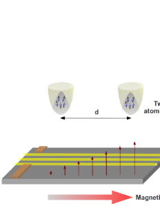
Figure 1: (Color online) Schematic of two atomic condensates being placed above a surface which produces a magnetic-field gradient. The two trapped condensates are separate with a distance $d$. The atoms are coupled to the magnetic fields through their magnetic dipoles.

II System

We consider two spatially separated Bose-Einstein condensates (BECs) of ⁸⁷Rb atoms, where each atom has two hyperfine levels $|e\rangle=|F=2,m_{F}^{\prime}\rangle$ and $|g\rangle=|F=1,m_{F}=-1\rangle$ Bohi . Here the magnetic number $m_{F}^{\prime}$ of the upper hyperfine level can be $-2$, $-1$ or $0$. This upper state $|e\rangle$ can be carefully chosen for which the polarization of the magnetic field is to be detected Bohi . The two BECs are placed above a surface which generates a magnetic-field gradient as shown in Fig. 1. The two condensates are coupled to the two different magnetic fields via their magnetic dipoles Bohi ; Ng1 .

We adopt the two-mode approximation Milburn to describe the atoms in deep potential wells. The Hamiltonian $H_{0}$ can be written as Ng2

$$H_{0} = -\frac{\hbar}{2}({E^{e}_{J}}e^{\dagger}_{L}e_{R}+{E^{g}_{J}}g^{\dagger}_{L}g_{R}+{\rm H.c})$$ (1)

$$+{\hbar}\sum_{\alpha={L,R}}(U_{ee}{n}^{2}_{e_{\alpha}}+2U_{eg}{n}_{e_{\alpha}}n_{g_{\alpha}}+U_{gg}n^{2}_{g_{\alpha}}),$$

where $e_{\alpha}(g_{\alpha})$ and $n_{e_{\alpha}}(n_{g_{\alpha}})$ are the annihilation and number operators of the atoms in the state $|e\rangle(|g\rangle)$ in the left and right potential wells, respectively. The parameters $E^{e}_{J}(E^{g}_{J})$ and $U_{ee}(U_{gg})$ are the tunneling strength between the two wells and the atom-atom interaction strength, for the states $|e\rangle(|g\rangle)$, and $U_{eg}$ is the interaction strength between the atoms in the two different components.

We consider the atoms to be resonantly coupled to the microwave magnetic fields. The transition frequencies of hyperfine states can be tuned by a static magnetic field Bohi . Here the other hyperfine transitions can be ignored due to large detuning Bohi . The Hamiltonian $H_{I}$, describes the internal states and their interactions between the magnetic fields, is given by Bohi

$$H_{I}=\hbar\sum_{\alpha=L,R}\Big{[}{\omega_{e}}n_{e\alpha}+{\omega_{g}}n_{g\alpha}+\frac{\Omega_{\alpha}}{2}(e^{i\omega{t}}e^{\dagger}_{\alpha}g_{\alpha}+{\rm H.c.})\Big{]},$$ (2)

where $\omega_{e}$ and $\omega_{g}$ are the frequencies of the atoms in the states $|e\rangle$ and $|g\rangle$, respectively, and $\omega$ is the frequency of the magnetic field. The parameter $\Omega_{L}(\Omega_{R}$) is the coupling strength between the atoms and magnetic field $B_{L}(B_{R}$) in the left(right) potential well.

We work in the interaction picture by performing the unitary transformation as

$$U(t) = \exp\Bigg{[}-it\sum_{\alpha=L,R}({\omega}n_{e\alpha}+\omega_{g}n_{g\alpha})\Bigg{]}.$$ (3)

The transformed Hamiltonian becomes

$$H_{I} = \hbar\sum_{\alpha=L,R}\Big{[}{\Delta}n_{e\alpha}+\frac{\Omega_{\alpha}}{2}(e^{\dagger}_{\alpha}g_{\alpha}+{\rm H.c.})\Big{]},$$ (4)

where $\Delta=\omega_{e}-\omega$ is the detuning between the atoms and the magnetic field.

If the two wells are separate with a large distance, then the tunneling strengths are effectively turned off, i.e., $E^{e}_{J}=E^{g}_{J}=0$. Here we consider the number of atoms in each trap to be equal to $N/2$, where $N$ is the total number of atoms. For convenience, the system can be expressed in terms of angular momentum operators as Sakurai :

$$J_{\alpha{x}} = \frac{1}{2}(e^{\dagger}_{\alpha}{g_{\alpha}}+g^{\dagger}_{\alpha}{e_{\alpha}}),$$ (5)

$$J_{\alpha{y}} = \frac{1}{2i}(e^{\dagger}_{\alpha}{g_{\alpha}}-g^{\dagger}_{\alpha}{e_{\alpha}}),$$ (6)

$$J_{\alpha{z}} = \frac{1}{2}(e^{\dagger}_{\alpha}{e_{\alpha}}-g^{\dagger}_{\alpha}{g_{\alpha}}),$$ (7)

where $\alpha=L,R$. The Hamiltonians $H_{0}$ and $H_{I}$ are rewritten as

$$H_{0} = \hbar\sum_{\alpha={L,R}}\Big{[}\frac{1}{2}(U_{ee}-U_{gg}){N}J_{\alpha{z}}+{\chi}J^{2}_{\alpha{z}}\Big{]},$$ (8)

$$H_{I} = {\hbar}\sum_{\alpha=L,R}(\Delta{J}_{\alpha{z}}+\Omega_{\alpha}{J}_{\alpha{x}}),$$ (9)

where $\chi=U_{ee}+U_{gg}-2U_{eg}$. We have omitted a constant term $\hbar(U_{ee}N^{2}+U_{gg}N^{2}+2U_{eg}N^{2}+4{\Delta}N)/8$.

III Detection of magnetic-field gradient

We present a scheme for detecting the magnetic-field gradient by using a pair of entangled BECs. First, it is necessary to generate the entanglement between two spatially separated condensates. Then, one of the condensates can be brought to another place for detection and the atoms are coupled to the magnetic fields. The magnetic-field gradient can be estimated by measuring the variances of the population differences and relative phases between the condensates in the two internal states. The procedure of this detection scheme is described in the following:

III.1 Generation of entangled states

To enhance the sensitivity of detection, it is necessary to generate the entanglement between the two separate condensates. We consider the condensates to be prepared in an entangled state which is given by Cable

$$|\Psi_{\rm in}\rangle = \frac{1}{\sqrt{2j+1}}\sum_{m}(-1)^{m}|j,m\rangle_{L}|j,-m\rangle_{R},$$ (10)

where $|j,m\rangle_{\alpha}$ is an eigenstate of angular momentum operator $J_{\alpha{z}}$ for $\alpha=L,R$, and $j=N/4$. The spin states of the two condensates are anti-correlated Ng2 .

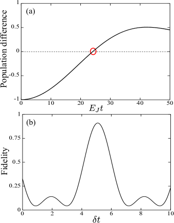
Figure 2: (Color online) (a) Time evolution of the population difference between two wells versus time, for the atoms in the state $|g\rangle$. (b) Fidelity between the input state $|\Psi_{\rm in}\rangle$ and the state $|\psi(t)\rangle$ versus time. The red circle denotes the zero population difference between the two wells at the time $t^{*}$. The parameters are used: $N=4$, $U=10E_{J}$, $\delta_{L}=\delta$ and $\delta_{R}=0$.

Now we discuss how to generate the entangled state $|\Psi_{\rm in}\rangle$ in Eq. (10). Initially, the atoms in the two different internal states $|e\rangle$ and $|g\rangle$ are confined in the different potential wells, respectively, where each condensate has an equal number of atoms, $N/2$. The intra- and inter-component interaction strengths are tuned to be the same, i.e., $U\!\approx\!U_{ee}\!\approx\!{U_{gg}}\!\approx\!U_{eg}/2$. The tunneling strengths $E_{J}\!\approx\!{E^{e}_{J}}\!\approx\!{E^{g}_{J}}$ are much weaker than the atomic interaction strengths $U$. The entanglement between the atoms in the two components can be dynamically produced via the process of tunneling Ng2 . In this process, the atoms in the two different internal states can tunnel in pair due to the strong atom-atom interactions. The entangled state can then be generated as Ng2

$$|\Psi(t^{*})\rangle\approx\sum_{n}{c_{n}}|n\rangle_{g_{L}}|N/2-n\rangle_{g_{R}}|N/2-n\rangle_{e_{L}}|n\rangle_{e_{R}},$$ (11)

where $c_{n}$ is the probability amplitude. When the population difference between the wells for each component condensate is about zero at the time $t^{*}$, the probability amplitude $c_{n}$ is approximately equal to $1/\sqrt{N/2+1}$. Then, the tunneling can be effectively switched off by adiabatically separating the two wells. Since the number of atoms in each well is equal to each other, the two-component condensate in each trap can be effectively described by an angular momentum system. Therefore, the state $|\Psi(t^{*})\rangle$ can be rewritten as Ng2

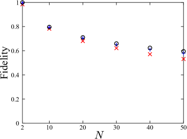
Figure 3: (Color online) Fidelity between the input state $|\Psi_{\rm in}\rangle$ and the entangled state $|\tilde{\Psi}\rangle$ versus the total number $N$ of atoms. The fidelities are shown with the different parameters for generating $|\tilde{\Psi}\rangle$: $U=5E_{J}$ (red cross), $10E_{J}$ (blue plus) and $50E_{J}$ (black empty circle), respectively.

$$|\Psi(t^{*})\rangle\! \approx \!\frac{1}{\sqrt{2j+1}}\!\sum_{m}\!|n\rangle_{g_{L}}|N/2-n\rangle_{e_{L}}|N/2-n\rangle_{g_{R}}|n\rangle_{e_{R}},$$ (12)

$$\approx \frac{1}{\sqrt{2j+1}}\sum_{m}|j,m\rangle_{L}|j,-m\rangle_{R},$$

where $|j,m\rangle_{L}=|n\rangle_{g_{L}}|N/2-n\rangle_{e_{L}}$ and $|j,-m\rangle_{R}=|N/2-n\rangle_{g_{R}}|n\rangle_{e_{R}}$ are the eigenstates of $J_{Lz}$ and $J_{Rz}$, respectively.

In Fig. 2(a), we plot the population difference between the two wells versus time, where the atoms are in $|g\rangle$. A red empty circle denotes the time $t^{*}$ for which the population difference is equal to zero. The atoms in $|g\rangle$ can tunnel to the other well even if the interaction strengths $U$ are much stronger than $E_{J}$.

The entangled state $|\Psi(t^{*})\rangle$ in Eq. (12) differs from the entangled state $|\Psi_{\rm in}\rangle$ in Eq. (10) in the relative phases between the atoms. A relative phase shift can be accumulated by turning on the interaction which can be described by the Hamiltonian $H_{\rm rp}$ as

$$H_{\rm rp} = \hbar(\delta_{L}J_{L{z}}+\delta_{R}J_{R{z}}),$$ (13)

where $\delta_{L}$ is not equal to $\delta_{R}$. The state $|\psi(t)\rangle$ can be produced as

$$|\psi(t)\rangle = \exp(-iH_{\rm rp}t)|\Psi(t^{*})\rangle.$$ (14)

This interaction can be made by controlling the strength $U_{ee}$ and $U_{gg}$ in Eq. (8) in one of the potential wells. Note that this interaction will not change the population difference between the two-component condensates. Therefore, the quantum numbers $m$ in Eq. (12) remain unchanged during the interaction. After turning on the interaction for a specific time, the required entangled state $|\tilde{\Psi}\rangle$ can then be produced, where $|\tilde{\Psi}\rangle$ is the state which has the maximum fidelity Uhlmann between $|\Psi_{\rm in}\rangle$ and $|\psi(t)\rangle$.

We then study the fidelity between the states $|\Psi_{\rm in}\rangle$ and $|\psi(t)\rangle$. In Fig. 2(b), we plot the fidelity, $|\langle\Psi_{\rm in}|\psi(t)\rangle|^{2}$, is plotted versus the time, where $\delta_{L}=\delta$ and $\delta_{R}=0$. The fidelity varies with the time $t$ as shown in Fig. 2(b). The highest fidelity can exceed 0.9.

In addition, we examine the fidelity between the states $|\Psi_{\rm in}\rangle$ and $|\tilde{\Psi}\rangle$ for the different numbers $N$ of atoms in Fig. 3. As $N$ increases, the fidelities decreases. However, the higher fidelity can be obtained with a higher ratio of $U$ to $E_{J}$.

III.2 Coupling to the magnetic field

We consider the atoms to be coupled to the magnetic field at resonance, i.e., $\Delta=0$ and set $U_{ee}=U_{gg}$. Here we assume that the strengths of atom-atom interactions are much weaker than the coupling strengths $\Omega_{L}$ and $\Omega_{R}$, and therefore they are ignored here. The effect of the atom-atom interactions will be discussed later. The Hamiltonian $H_{I}$ reads

$$H_{I} = {\hbar}(\Omega_{L}{J}_{L{x}}+\Omega_{R}{J}_{R{x}}).$$ (15)

The magnetic coupling strengths $\Omega_{L}$ and $\Omega_{R}$ are different to each other. Let us write $\Omega_{L}=\Omega+\Omega_{D}/2$ and $\Omega_{R}=\Omega-\Omega_{D}/2$. The Hamiltonian $H_{I}$ can be written as

$$H_{1} = {\hbar}\Omega({J}_{L{x}}+{J}_{R{x}})+\frac{\hbar\Omega_{D}}{2}({J}_{L{x}}-{J}_{R{x}}).$$ (16)

This small parameter $\Omega_{D}$ is to be determined.

III.3 Read-out process

The magnetic-field gradient can be estimated by measuring the variance $\langle\tilde{J}^{2}_{yz}\rangle=\langle{J^{2}_{y-}-J^{2}_{z+}}\rangle$, where $J_{y-}=J_{Ly}-J_{Ry}$ and $J_{z+}=J_{Lz}+J_{Rz}$. Physically speaking, $\langle{J_{\alpha{y}}}\rangle$ and $\langle{J_{\alpha{z}}}\rangle$ are the expectation values of the relative phase and population difference between the two-component condensates in the potential well $\alpha$, for $\alpha=L,R$. The variance $\langle\tilde{J}^{2}_{yz}\rangle$ is given by

$$\langle{\tilde{J}^{2}_{yz}}(\phi_{D})\rangle = \frac{N(N+4)}{12}\cos{(\phi_{D})}.$$ (17)

where $\phi_{D}=\Omega_{D}t$. Here $\langle{J_{y-}}\rangle$ and $\langle{J_{z+}}\rangle$ are equal to zero for the input state $|\Psi_{\rm in}\rangle$ in Eq. (10). The expectation value $\langle{\tilde{J}^{2}_{yz}(\phi_{D})}\rangle$ is a function of the parameter $\phi_{D}$. Therefore, this quantity can be used for determining the magnetic-field gradient $\Omega_{D}$.

Figure 4: (Color online) The variances $\langle\tilde{J}^{2}_{yz}\rangle$ are plotted versus time, for $N=4$ and $\Omega_{D}=0.05\Omega$. The black solid and blue dotted lines are shown by using the two different initial states $|\Psi_{\rm in}\rangle$ and $|\tilde{\Psi}\rangle$, respectively, where $U=10E_{J}$ is used for producing $|\tilde{\Psi}\rangle$.

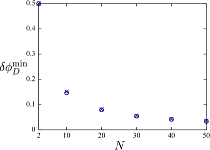
Figure 5: (Color online) The minimum of the uncertainties $\delta\phi^{\rm min}_{D}$ versus the total number $N$ of atoms, for $\Omega_{D}=0.05\Omega$. The empty circles and blue crosses denote the system with the two different initial states $|\Psi_{\rm in}\rangle$ and $|\tilde{\Psi}\rangle$, respectively, where $U=10E_{J}$ is used for producing the state $|\tilde{\Psi}\rangle$.

In Fig. 4, we plot the variance $\langle\tilde{J}^{2}_{yz}\rangle$ versus the time, for the two different initial states $|\Psi_{\rm in}\rangle$ and $|\tilde{\Psi}\rangle$, respectively. The variances $\langle\tilde{J}^{2}_{yz}\rangle$ oscillate with the frequency $\phi_{D}$, for these two initial states. But the variance $\langle\tilde{J}^{2}_{yz}\rangle$ shows some small-amplitude fluctuations in the slow oscillations if the initial state $|\tilde{\Psi}\rangle$ is used.

III.4 Sensitivity of detection

The magnetic-field gradient can be estimated from the variance $\langle\tilde{J}^{2}_{yz}\rangle$. The uncertainty of the parameter $\phi_{D}$ is given by

$$\delta{\phi}_{D} =\dfrac{\Delta{\tilde{J}^{2}_{yz}}}{|\partial\langle{\tilde{J}^{2}_{yz}}\rangle/\partial\phi_{D}|},$$ (18)

where $\Delta{\tilde{J}^{2}_{yz}}=\sqrt{\langle\tilde{J}^{4}_{yz}\rangle-\langle{\tilde{J}^{2}_{yz}}\rangle^{2}}$. The uncertainty $\delta\phi_{D}$ can be found as

$$\delta\phi_{D}=\sqrt{\frac{15\sin^{2}(\phi_{D})+(N-2)(N+6)\cos^{2}({\phi_{D})}}{5N(N+4)\sin^{2}(\phi_{D})}}.$$ (19)

At the time $t=\pi/2\Omega_{D}$, the minimum uncertainty $\delta\phi^{\rm min}_{D}$ is

$$\delta\phi^{\rm min}_{D} = \sqrt{\frac{3}{N(N+4)}}.$$ (20)

The uncertainty scales with $1/N$, for large $N$. Thus, the accuracy of measurement can reach the Heisenberg limit Giovannetti .

In Fig. 5, we plot the minimum uncertainties $\delta\phi^{\rm min}_{D}$ versus the total number of atom, for the two different initial states $|\Psi_{\rm in}\rangle$ and $|\tilde{\Psi}\rangle$, respectively. The measurement using the two different initial states can give the similar values of $\delta\phi^{\rm min}_{D}$. Therefore, the entangled state $|\tilde{\Psi}\rangle$ can provide a similar accuracy of the case using the input state $|\Psi_{\rm in}\rangle$ in Eq. (10).

IV Effect of atom losses

Now we study the sensitivity of the detection in the presence of one-body and two-body atom losses.

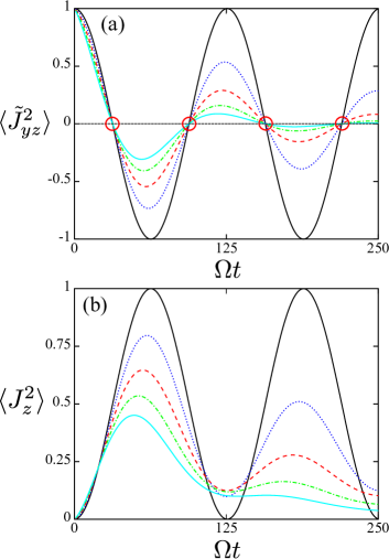
Figure 6: (Color online) (a) Variances $\langle\tilde{J}^{2}_{yz}\rangle$ versus time. (b) Variances $\langle{J}^{2}_{z}\rangle$ versus time. The initial state is the entangled state $|\Psi_{\rm in}\rangle$ in Eq. (10). The parameters are used: $\Omega_{D}=0.05\Omega$ and $N=2$. The different damping rates are shown: $\gamma^{o}=0$ (black solid line), $0.0025\Omega$ (blue dotted line), $0.005\Omega$ (red dashed line), $0.0075\Omega$ (green dot-dashed line) and $0.01\Omega$ (cyan solid line), respectively. The red empty circles denote the intersection points at $\langle\tilde{J}^{2}_{yz}\rangle=0$.

IV.1 One-body atom loss

Here we study the one-body atom losses by using the phenomenological master equation Cooper1 ; Cooper2 . The master equation, describes one-body atom losses, can be written as Cooper1 ; Cooper2

$$\dot{\rho}=i[\rho,H]+\sum_{\alpha,\beta}\frac{\gamma^{o}_{\beta}}{2}(2\beta_{\alpha}\rho\beta^{\dagger}_{\alpha}-\beta^{\dagger}_{\alpha}\beta_{\alpha}\rho-\rho\beta^{\dagger}_{\alpha}\beta_{\alpha}),$$ (21)

where $\gamma^{o}_{\beta}$ is the damping rate of one-body atom loss, and $\alpha=L,R$ and $\beta=e,g$.

We compare the two estimators $\langle\tilde{J}^{2}_{yz}\rangle$ and $\langle{J}^{2}_{z}\rangle$ for determining the parameter $\phi_{D}$ in the presence of one-body atom loss, where $J_{z}=J_{Lz}+J_{Rz}$ is the sum of the population difference between the two hyperfine spin states of condensates in the two wells. In Fig. 6(a), we plot the variance $\langle\tilde{J}^{2}_{yz}\rangle$ versus time for the different damping rates $\gamma^{o}=\gamma^{o}_{e}=\gamma^{o}_{g}$.

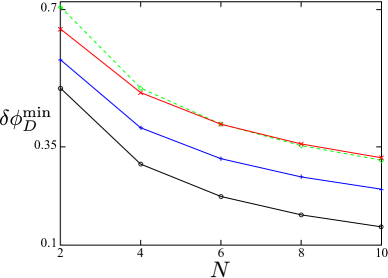
Figure 7: (Color online) The minimum uncertainties $\delta\phi^{\rm min}_{D}$ are plotted versus $N$ for $\Omega_{D}=0.05\Omega$. The different damping rates are shown: $\gamma^{o}=0$ (black empty circle), $0.005\Omega$ (blue plus) and $0.01\Omega$ (red cross), respectively. The green diamonds (dashed line) denote the case of using uncorrelated atoms with the uncertainty, $1/\sqrt{N}$, for $\gamma^{o}=0$.

The initial state is $|\Psi_{\rm in}\rangle$ in Eq. (10). We can see that the variances $\langle\tilde{J}^{2}_{yz}\rangle$ intersect at the same point at the time $t=n\pi/2\Omega_{D}$, where $n$ is an odd number. The parameter $\Omega_{D}$ can be estimated in the vicinity of these intersection points. In fact, the minimum uncertainty of the parameter $\Omega_{D}$ can be obtained at the first intersection point, i.e., $t=\pi/2\Omega_{D}$.

In Fig. 6(b), the variances $\langle{J}^{2}_{z}\rangle$ are plotted versus time, for the different damping rates $\gamma^{o}$. For $\gamma^{o}=0$, the variance $\langle{J^{2}_{z}}\rangle$ can be used for determining the parameter $\Omega_{D}$ Lanz . However, the estimators $\langle{J}^{2}_{z}\rangle$ do not intersect at the same point for the different damping rates $\gamma^{o}$. Besides, the atom losses cause a shift of the oscillations. This means that $\langle{J}^{2}_{z}\rangle$ is not a faithful estimator for determining the parameter $\Omega_{D}$ in the presence of atom losses.

In Fig. 7, we plot the minimum uncertainties $\delta\phi^{\rm min}_{D}$ versus the total number $N$ of atoms, where $N$ is up to 10. Here the minimum uncertainty $\delta\phi^{\rm min}_{D}$ are obtained at the time $t=\pi/2\Omega_{D}$. For comparsion, the case using uncorrelated atoms without any atom loss is shown (green diamonds in Fig. 7), where the uncertainty is equal to $1/\sqrt{N}$ Giovannetti . In Fig. 7, the entangled atoms can give a better performance than the uncorrelated atoms in detection if the damping rate $\gamma^{o}$ is much smaller than $\Omega_{D}=0.05\Omega$. When $\gamma^{o}=0.01\Omega$ becomes comparable to $\Omega_{D}$, the accuracy of the detection is similar to the case using uncorrelated atoms as shown in Fig. 7.

IV.2 Two-body atom loss

The phenomenological master equation, describes two-body atom losses, can be written as Rey

$$\dot{\rho} = \!i[\rho,H]\!+\frac{\gamma^{t}_{ee}}{2}\!\!\sum_{\alpha=L,R}\!(2e^{2}_{\alpha}{\rho}{e^{{\dagger}{2}}_{\alpha}}-e^{{\dagger}{2}}_{\alpha}{e}^{2}_{\alpha}\rho-\rho{e}^{{\dagger}{2}}_{\alpha}{e}^{2}_{\alpha})$$

$$+\frac{\gamma^{t}_{eg}}{2}\!\!\sum_{\alpha=L,R}\!(2e_{\alpha}{g_{\alpha}}{\rho}e^{\dagger}_{\alpha}{g^{\dagger}_{\alpha}}-e^{\dagger}_{\alpha}{e}_{\alpha}{g^{\dagger}_{\alpha}{g}_{\alpha}}\rho-\rho{e}^{\dagger}_{\alpha}{e}_{\alpha}{g^{\dagger}_{\alpha}{g}_{\alpha}}),$$

where the parameters $\gamma^{t}_{ee}$ and $\gamma^{t}_{eg}$ are the damping rates of two-body atom losses for the condensates in the upper internal state $|e\rangle$ and the atoms in the two different components, and $\alpha=L,R$.

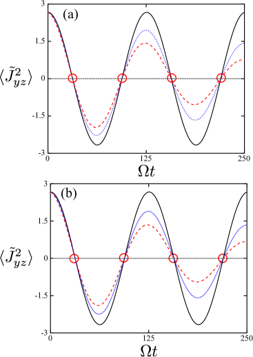
Figure 8: (Color online) Variances $\langle\tilde{J}^{2}_{yz}\rangle$ versus time. (a) The different damping rates are shown: $\gamma^{t}_{eg}=0$ (black solid line), $0.005\Omega$ (blue dotted line) and $0.01\Omega$ (red dashed line), respectively, and $\gamma^{t}_{ee}=0$. (b) The different damping rates are shown: $\gamma^{t}_{eg}=0$ (black solid line), $0.001\Omega$ (blue dotted line) and $0.002\Omega$ (red dashed line), respectively, and $\gamma^{t}_{ee}=1.5\gamma^{t}_{eg}$. The initial state is the input state $|\Psi_{\rm in}\rangle$. The parameters are used: $\Omega_{D}=0.05\Omega$ and $N=4$. The red empty circles denote the intersection points at $\langle\tilde{J}^{2}_{yz}\rangle=0$.

In Fig. 8(a) and (b), we plot the estimators $\langle\tilde{J}^{2}_{yz}\rangle$ versus time, for the different damping rates $\gamma^{t}_{eg}$ of two-body atom losses, and $\gamma^{t}_{ee}=0$ in (a) and $\gamma^{t}_{ee}=1.5\gamma^{t}_{eg}$ Mertes in (b), respectively. Both of the results show that $\langle\tilde{J}^{2}_{yz}\rangle$ intersect at the times $n\pi/2\Omega_{D}$, where $n$ is an odd number. Therefore, the parameter $\Omega_{D}$ can be estimated at the times $n\pi/2\Omega_{D}$ in the presence of two-body atom losses.

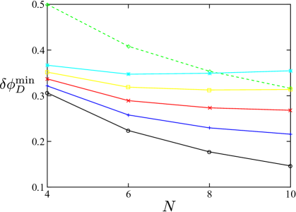
Figure 9: (Color online) The minimum uncertainties $\delta\phi^{\rm min}_{D}$ versus $N$ for $\Omega_{D}=0.05\Omega$. The different damping rates $\gamma^{t}_{eg}$ are shown: $\gamma^{t}_{eg}=0$ (black empty circle), $0.0025\Omega$ (blue plus), $0.005\Omega$ (red cross), $0.0075\Omega$ (yellow square), $0.01\Omega$ (cyan star) respectively. The green diamonds (dashed line) denote the uncertainty, $1/\sqrt{N}$, by using uncorrelated atoms without any atom loss.

In Fig. 9, we plot the minimum uncertainties $\delta\phi^{\rm min}_{D}$ versus $N$, where the minimum uncertainties are taken at the time $t=\pi/2\Omega_{D}$. The uncertainties from the measurement with uncorrelated atoms are shown with green diamonds, where $\gamma^{t}_{eg}=\gamma^{t}_{ee}=0$. The parameters $\delta\phi^{\rm min}_{D}$ have the different scalings with $N$, for the different rates $\gamma^{t}_{eg}$ and $\gamma^{t}_{ee}=0$. For small $\gamma^{t}_{eg}$, the entangled atoms can outperform the uncorrelated atoms for detection. When $\gamma^{t}_{eg}\geq{0.0075\Omega}$ and $N\geq{8}$, the uncertainty $\delta\phi^{\rm min}_{D}$ does not decrease with $N$. To obtain the good performance of the measurements, the damping rates $\gamma^{t}_{eg}$ have to be much smaller than the coupling strength of the magnetic-field gradient.

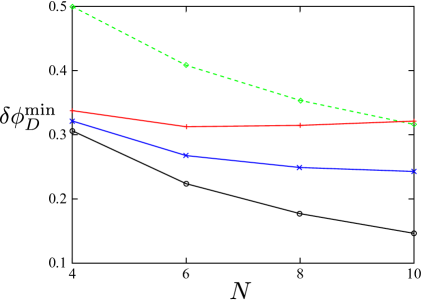
Figure 10: (Color online) The minimum uncertainties $\delta\phi^{\rm min}_{D}$ versus $N$, for $\Omega_{D}=0.05\Omega$. The different damping rates are shown: $\gamma^{t}_{eg}=0$ (black empty circle), $\gamma^{t}_{eg}=0.001\Omega$ (blue cross) and $\gamma^{t}_{eg}=0.002\Omega$ (red plus), respectively, for $\gamma^{t}_{ee}=1.5\gamma^{t}_{eg}$. The green diamonds (dashed line) denote the case of using uncorrelated atoms with the uncertainty, $1/\sqrt{N}$.

Then, we study the sensitivity of the detection by including the two-body atom loss for the atoms in the excited states in $|e\rangle$ Mertes . In Fig. 10, we plot the minimum uncertainty $\delta\phi^{\rm min}_{D}$ versus $N$, where the minimum uncertainties are taken at the time $t=\pi/2\Omega_{D}$. Here we set $\gamma^{t}_{ee}=1.5\gamma^{t}_{eg}$ Mertes . The minimum uncertainty exceeds the case of using uncorrelated atoms when $\gamma^{t}_{eg}$ is equal to $0.002\Omega$. In this case, the two-body atom losses become more detrimental to the performance of the detection.

V Effect of atom-atom interactions

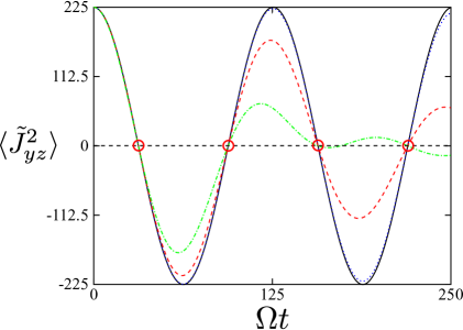
Figure 11: (Color online) Time evolution of variances $\langle\tilde{J}^{2}_{yz}\rangle$, for different strengths of atom-atom interactions: $\chi=0$ (black-solid line), $10^{-4}\Omega$ (blue-dotted line), $5\times{10^{-4}}\Omega$ (red-dashed line) and $0.001\Omega$ (green-dot-dashed line), respectively. The parameters are used: $N=50$ and $\Omega_{D}=0.05\Omega$. The red empty circles denote the intersection points at $\langle\tilde{J}^{2}_{yz}\rangle=0$.

We investigate the effect of the atom-atom interactions on the detection of magnetic-field gradient. In Fig. 11, we plot the variances $\langle\tilde{J}^{2}_{yz}\rangle$ versus time, for the different nonlinear interaction strengths $\chi$. When $\chi{N}\ll{\Omega}_{D}$, $\langle\tilde{J}^{2}_{yz}(t)\rangle$ are close to each other, for the different strengths $\chi$. If the nonlinear interaction strength $\chi$ increases, then the amplitude of oscillations decreases as shown in Fig. 11. In addition, the variances $\langle\tilde{J}^{2}_{yz}(t)\rangle$, for $\chi{N}{\ll}\Omega_{D}$, almost meet at the same points $\langle\tilde{J}^{2}_{yz}\rangle=0$ at the times $t=n\pi/2\Omega_{D}$, where $n$ is an odd number. At the times $n\pi/2\Omega_{D}$, these give the minimum uncertainty of the parameter $\phi_{D}$.

Then, we investigate the uncertainty $\delta\phi^{*}_{D}$ at the time $t=\pi/2\Omega_{D}$. In Fig. 12, we plot the uncertainties $\delta\phi^{*}_{D}$ versus $N$, for the different nonlinear interaction strengths $\chi$. The uncertainty $\delta\phi^{*}_{D}$ is close to the minimum uncertainty $\delta\phi^{\rm min}_{D}$ for $\chi{N}\ll{\Omega_{D}}$. When $\chi$ increases, the uncertainty $\delta\phi^{*}_{D}$ does not decrease for larger $N$ as shown in Fig. 12. Therefore, the strong nonlinear interactions limit the performance of detection.

In fact, the effects of nonlinear interactions can be minimized by setting $\chi{N}{\ll}\Omega_{D}$. The nonlinear interaction strength can be appropriately adjusted by using Feshbach resonance Gross and state-dependent trap Riedel .

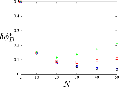
Figure 12: (Color online) The uncertainties $\delta\phi^{*}_{D}$ are plotted versus $N$, for $\delta\Omega_{D}=0.05\Omega$. The different strengths of atom-atom interactions are shown: $\chi=0$ (black empty circle), $10^{-4}\Omega$ (blue cross), $5\times{10^{-4}}\Omega$ (red square) and $0.001\Omega$ (green plus), respectively.

VI Discussion

Let us make some remarks on our method for detecting the magnetic-field gradient by using ⁸⁷Rb atoms. The transition frequency of ⁸⁷Rb atoms can be tuned by using an external static magnetic field Bohi , the range of the frequencies of the detected magnetic field is about a few GHz to 10 GHz Bohi ; Steck .

Next, we roughly estimate the magnitude of the magnetic-field gradient which can be probed by using the condensates. Indeed, the measurement is mainly limited by the atom loss rate of the condensates. The main source comes from two-body atom losses Mertes . The two-body loss rate $(\gamma^{t}_{eg}+\gamma^{t}_{ee})N/V$, where $\gamma^{t}_{eg}(\gamma^{t}_{ee})\sim{10^{-13}}{\rm cm}^{3}{\rm s}^{-1}$ Mertes and $V$ is the volume of the condensate. The rates of two-body atom losses depend on the density of the atomic gases. We assume that $V$ is about $(1\mu{\rm m})^{3}$. The rates of two-body atom loss range from 1 Hz to 10 Hz, for $N={10}$ to 100. To obtain the good performance, the coupling strength of the magnetic-field gradient $\Omega_{D}$ must be much larger than the two-body atom loss rates. The coupling strength $\Omega_{L(R)}$ between the two states is about $\mu_{B}{B}_{L(R)}/\hbar$ Bohi , where $\mu_{B}$ is the Bohr magneton. Thus, the minimum value of magnetic field can be detected ranging from $10^{-10}$T to $10^{-9}$T, for $N=10$ to 100 and $V=(1\mu{\rm m})^{3}$. The minimum value of the detectable magnetic-field gradient is about $10^{-9}{\sim}10^{-10}$T.

VII Conclusion

In summary, we have proposed a method to detect the magnetic-field gradient by using entangled condensates. We have described how to generate entangled states of two spatially separated condensates. The magnetic-field gradient can be determined by measuring the variances of relative phases and population differences between the two-component condensates in the two wells. The uncertainty of the parameter scales with $1/N$. We have also numerically studied the effects of one-body and two-body atom losses on the detection. We show that the entangled atoms can outperform the uncorrelated atoms in detecting the magnetic fields for a few atoms. The effect of atom-atom interactions on this method has also been discussed.

- (1) D. Budker and M. Romalis, Nat. Phys. 3, 227 (2007).
- (2) Y. S. Greenberg, Rev. Mod. Phys. 70, 175 (1998).
- (3) M. Hämääinen, R. Hari, R. J. Ilmoniemi, J. Knuutila, and O. V. Lounasmaa, Rev. Mod. Phys. 65, 413 (1993).
- (4) S. Wildermuth, S. Hofferberth, I. Lesanovsky, S. Groth, P. Krüger, and J. Schmiedmayer, Appl. Phys. Lett. 88, 264103 (2006).
- (5) M. Vengalattore, J. M. Higbie, S. R. Leslie, J. Guzman, L. E. Sadler, and D. M. Stamper-Kurn, Phys. Rev. Lett. 98, 200801 (2007).
- (6) P. Böhi, M. F. Riedel, T. W. Hänsch, P. Treutlein, Appl. Phys. Lett. 97, 051101 (2010) .
- (7) D. M. Harber, H. J. Lewandowski, J. M. McGuirk, and E. A. Cornell, Phys. Rev. A 66, 053616 (2002).
- (8) P. Treutlein, P. Hommelhoff, T. Steinmetz, T. W. H’́ansch, and J. Reichel, Phys. Rev. Lett. 92, 203005 (2004)
- (9) R. Horodecki, P. Horodecki, M. Horodecki, and K. Horodecki, Rev. Mod. Phys. 81, 865 (2009).
- (10) V. Giovannetti, S. Lloyd, L. Maccone, Science 306, 1330 (2004).
- (11) C. Gross, T. Zibold, E. Nicklas, J. Estev̀e and M. K. Oberthaler, Nature 464, 1165 (2010).
- (12) M. F. Riedel, P. Boḧi, Y. Li, T. W. Han̈sch, A. Sinatra and P. Treutlein, Nature 464, 1170 (2010).
- (13) H. T. Ng and Shih-I Chu, Phys. Rev. A 84, 023629 (2011).
- (14) P. Hommelhoff, W. Hänsel, T. Steinmetz, T. W. Hänsch and J. Reichel, New J. Phys. 7, 3 (2005).
- (15) A. Sørensen, L.-M. Duan, J. I. Cirac and P. Zoller, Nature 409, 63 (2001).
- (16) H. Cable and G. A. Durkin, Phys. Rev. Lett. 105, 013603 (2010).
- (17) I. Urizar-Lanz, P. Hyllus, I. L. Egusquiza, M. W. Mitchell, and G. Tóth, arXiv:1203.3797.
- (18) H. T. Ng, C. K. Law, and P. T. Leung, Phys. Rev. A 68, 013604 (2003).
- (19) M. Albiez, R. Gati, J. Fölling, S. Hunsmann, M. Cristiani and M. K. Oberthaler, Phys. Rev. Lett. 95, 010402 (2005).
- (20) S. Fölling, S. Trotzky, P. Cheinet, M. Feld, R. Saers, A. Widera, T. Müller and I. Bloch, Nature 448, 1029 (2007).
- (21) J. Estève, C. Gross, A. Weller, S. Giovanazzi and M. K. Oberthaler, Nature 455, 1216 (2008).
- (22) J. J. Cooper, D. W. Hallwood, and J. A. Dunningham, Phys. Rev. A 81, 043624 (2010).
- (23) J. J. Cooper, D. W. Hallwood, J. A. Dunningham, and J. Brand, Phys. Rev. Lett. 108, 130402 (2012).
- (24) A. M. Rey, L. Jiang, and M. D. Lukin, Phys. Rev. A 76, 053617 (2007).
- (25) K. M. Mertes, J.W. Merrill, R. Carretero-Gonzàlez, D. J. Frantzeskakis, P. G. Kevrekidis, and D. S. Hall, Phys. Rev. Lett. 99, 190402 (2007).
- (26) J. Grond, U. Hohenester, I. Mazets and J. Schmiedmayer, New J. Phys. 12, 065036 (2010).
- (27) I. Tikhonenkov, M. G. Moore, and A. Vardi, Phys. Rev. A 82, 043624 (2010).
- (28) G. J. Milburn, J. Corney, E. M. Wright, and D. F. Walls, Phys. Rev. A 55, 4318 (1997).
- (29) J. J. Sakurai, Modern Quantum Mechanics (Addison-Wesley, Reading, MA, 1994).
- (30) A. Uhlmann, Rep. Math. Phys. 9, 273 (1976); R. Jozsa, J. Mod. Opt. 41, 2315 (1994).
- (31) D. A. Steck, Rubidium 87 D line data, [http://steck.us/alkalidata/]