Modified Associate Formalism without Entropy Paradox:
Part II. Comparison with Similar Models

Abstract

The modified associate formalism is compared with similar models, such as the classical associate model, the associate species model and the modified quasichemical model. Advantages of the modified associate formalism are demonstrated.

,

1 Introduction

In this paper we compare the modified associate formalism (MAF) proposed in the first paper [1] with the classical associate model (CAM) described by Prigogine and Defay [2] and the associate species model (ASM) described by Besmann and Spear [3]. Where it is possible, we compare MAF with the classical quasichemical model (CQM) of Fowler and Guggenheim [4]. We also compare MAF with two modifications of CQM. The first modification suggested by Pelton and Blander [5] include:

• selection of the coordination numbers that allow one to set the composition of maximum ordering so as to comply with the experimental data;

• an empirical expansion of the molar Gibbs energy of the quasichemical reaction as polynomials in terms of coordination equivalent mole fractions of solution components, which is used for fitting available experimental data.

The first version of the modified quasichemical model is referred to as MQM(1986) in the present study. Further modifications of the quasichemical model introduced by Pelton et al. [6] are:

• expansion of the Gibbs energy of the quasichemical reaction as polynomials in pair fractions (instead of equivalent mole fractions of solution components), which provides advantages in data-fitting;

• dependence of coordination numbers of the solution components on the mole numbers of different pairs that allow one to set the composition of maximum ordering so as to comply with the experimental data for each binary system individually.

We refer to the second version of the modified quasichemical model as MQM(2000).

2 Configurational Entropy of Mixing in Binary Solutions

In this section, we compare the molar configurational entropies of mixing given by the solution models mentioned above with theoretical boundaries for the configurational entropy of mixing. These boundaries are discussed immediately below.

The configurational entropy of mixing is a measure of disorder and has its maximum value for an ideal solution which is completely disordered. For any solid or liquid solution $A-B$, the configurational entropy of mixing can not exceed that of ideal solution. On the other hand, when vacancies are not taken into account (which is the case in all considered models), the configurational entropy of mixing can not be negative. The values of molar configurational entropy of mixing which are outside of these boundaries are paradoxical.

For each model, we consider the following three limiting cases.

1. The case of ideal solution of $A$-particles and $B$-particles. In this case, the Gibbs free energy changes on forming associates that consist of both $A$-particles and $B$-particles. The configurational entropy of mixing should reduce to that of the ideal solution model.

2. The case of immiscible components $A$ and $B$. In this case, the configurational entropy of mixing should equals to zero.

3. The case of the highly ordered solution $A-B$. In this case, the Gibbs free energy change on forming of the associates of a particular composition and of a particular spacial arrangement of particles approaches $-\infty$. If the quasichemecal model is considered, the Gibbs free energy change on forming $(A-B)$-bonds approaches $-\infty$. The configurational entropy of mixing should be equal to zero at the composition of maximum ordering.

2.1 Classical Associate Model

Consider a solution of $x_{A}$ moles of the component $A$ and $x_{B}=1-x_{A}$ moles of the component $B$. The molar configurational entropy of mixing $s_{\text{conf}}$ given by the classical associate model [2] is expressed as

$$s_{\text{conf}}=-R(n_{A_{1}}\ln(x_{A_{1}})+n_{B_{1}}\ln(x_{B_{1}})+\sum\limits_{i,j\geq 1}n_{A_{i}B_{j}}\ln(x_{A_{i}B_{j}})).$$ (1)

Here, $n_{A_{1}}$, $n_{B_{1}}$ and $n_{A_{i}B_{j}}$ are the mole numbers (in one mole of the solution $A-B$), while $x_{A_{1}}$, $x_{B_{1}}$ and $x_{A_{i}B_{j}}$ are the molar fractions of $A_{1}$-monoparticles, $B_{1}$-monoparticles and ${A_{i}B_{j}}$-associates, respectively; $R$ is the universal gas constant. Note that compositions of associates and sizes of associates ($i+j$) are determined by a modeller. The equilibrium values of the mole numbers are determined by minimisation of the Gibbs free energy of the solution subject to the mass balance and nonnegativity constraints (see, for example, the monograph by Prigogine and Defay [2] for more details).

Now consider the limit when the Gibbs free energy changes on forming the associates equal to zero. As pointed out by Lück et al. [7], the classical associate model gives paradoxical values of the molar configurational entropy of mixing, which are larger than those given by the ideal solution model. Fig. 1, for example, shows the configurational entropy curves given by the classical associate model where only $A_{2}B$-associates are considered (solid line) and where $A_{2}B$-associates and $AB_{2}$-associates are considered (dashed line).

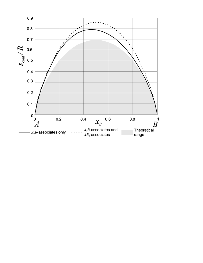
Figure 1: Molar configurational entropy of mixing given by the classical associate model in the limit of ideal solution of $A$-particles and $B$-particles.

As shown in the figure, the curves are outside of the theoretically possible range. Note also that the entropy curve is not symmetric with respect to vertical line with $x_{B}=1/2$ when only $A_{2}B$-associates are considered. To obtain a symmetric entropy curve (which is expected in the limit of ideal solution) one should consider both $A_{2}B$-associates and $AB_{2}$-associates.

Consider the limit when the Gibbs free energy changes on forming all associates approach $+\infty$. In this case, no associates form and the configurational entropy of mixing equals to that of the ideal solution model. In theory, however, the configurational entropy of mixing should be zero for any $x_{B}$.

Now consider the limit of highly ordered solution and assume that the Gibbs free energy change of forming $A_{2}B$-associates approaches $-\infty$. The entropy curve given by the classical associate model in this case is shown in Fig. 2. As shown in this figure, the entire entropy curve is within the theoretically possible range. Note also that the configurational entropy of mixing equals to zero at the composition of maximum ordering, since different spatial arrangements of particles in an $A_{2}B$-associate are not considered in the classical associate model.

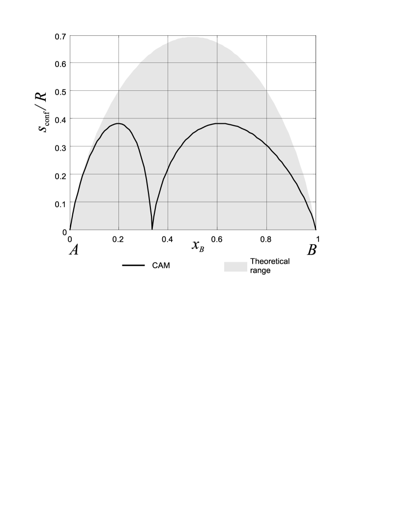
Figure 2: Molar configurational entropy of mixing given by the classical associate model in the limit of the highly ordered solution.

2.2 Associate Species Model

According to the associate species model [3], the configurational entropy of mixing of $x_{A}$ moles of the component $A$ and $x_{B}=1-x_{A}$ moles of the component $B$ is given by

$$s_{\text{conf}}=-\frac{R}{q}\left(\sum\limits_{a+b=1}n_{A_{a\cdot q}B_{b\cdot q}}\ln(x_{A_{a\cdot q}B_{b\cdot q}})\right).$$ (2)

Here, $q$ is the size of species (the number of particles per an associate specie); $n_{A_{a\cdot q}B_{b\cdot q}}$ are the mole numbers and $x_{A_{a\cdot q}B_{b\cdot q}}$ are the molar fractions of the ${A_{a\cdot q}B_{b\cdot q}}$-species. Similar to the classical associate model, the size and compositions of species are determined by a modeller.

Consider the limit of ideal solution, assuming that the solution consists of the associate species $A_{q}$, $B_{q}$, $A_{2q/3}B_{q/3}$ and $A_{q/3}B_{2q/3}$. The Fig. 3 shows the entropy curves given by the associate species model for $q=1$, $q=2$ and $q=3$. In contrast to the classical associate model, one can adjust the configurational entropy of mixing, using the additional parameter $q$. For this particular set of species, the selection of $q=2$ result in the entropy curve which is closed (though located outside the theoretically possible range) to the entropy curve given by the ideal solution model. As shown in Fig.  3, the selection $q=1$ results in substantial overestimation of the configurational entropy of mixing, while the selection $q=3$ gives underestimated values.

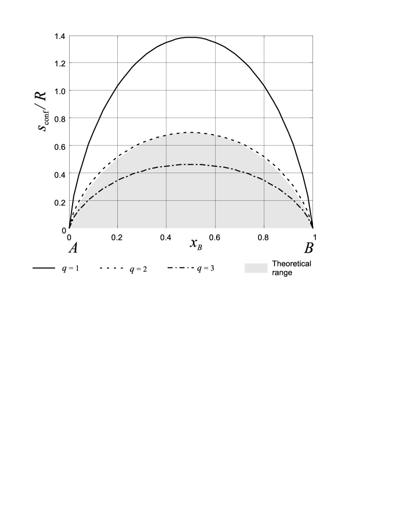
Figure 3: Molar configurational entropy of mixing given by the associate species model with the species $A_{q}$, $B_{q}$, $A_{2q/3}B_{q/3}$ and $A_{q/3}B_{2q/3}$ in the limit of ideal solution.

Consider the limit of immiscible components, that is, the Gibbs free energy changes on forming the species $A_{2q/3}B_{q/3}$ and $A_{q/3}B_{2q/3}$ approach $+\infty$. The entropy curves given by the associate species model in this case are shown in Fig. 4. As shown in this figure, the associate species model overestimate the configurational entropy of mixing in the limit of immiscible components. However, the entropy curve tends to theoretically expected one ($s_{\text{conf}}\equiv 0$), when $q$ increases.

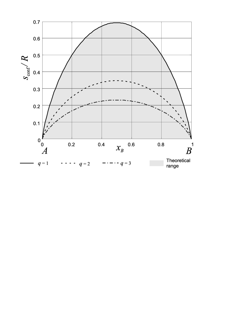
Figure 4: Molar configurational entropy of mixing given by the associate species model in the limit of immiscible components.

Now consider the limit of highly ordered solution. Assume also that the Gibbs free energy change on forming the associate species $A_{2q/3}B_{q/3}$ approaches $-\infty$. Fig. 5 shows the entropy curve given by the associate species model in this case. As seen from Fig. 5, the entropy curve with $q=3$ is entirely located in the theoretically possible range. If $q=2$, however, small part of the entropy curve (approximately, for $0<x_{B}<0.075$) is located outside the theoretically possible range. The selection $q=1$ results in paradoxical values of configurational entropy approximately for $0<x_{B}<0.25$ and $0.6<x_{B}<1$.

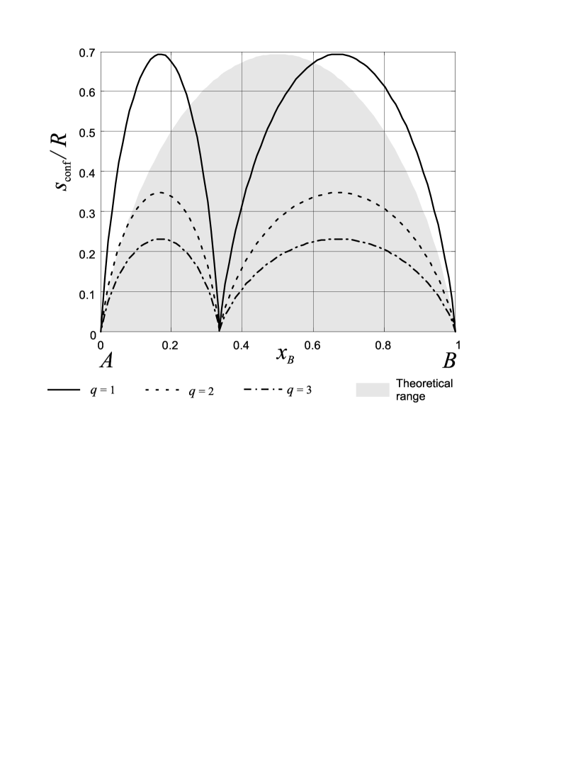
Figure 5: Molar configurational entropy of mixing given by the associate species model in the limit of highly ordered solution.

2.3 Modified Associate Formalism

In the modified associate formalism the configurational entropy of mixing is given by (see Eq. (44) in Ref. [1])

$$s_{\text{conf}}=-R\sum\limits_{{k_{1},\dots,k_{r}}\in{\mathfrak{S}_{m}}}\sum\limits_{j=1}^{J_{k_{1},\dots,k_{r}}}n_{k_{1},\dots,k_{r}}^{[j]}\ln\left(\frac{x_{k_{1},\dots,k_{r}}^{[j]}}{d_{k_{1},\dots,k_{r}}^{[j]}}\right)~{},$$ (3)

where all the notations have the same meaning as in Ref. [1]. In contrast to previous modifications of the associate model, the compositions of associates that have to be considered are defined by the size of associates.

Consider the limit of ideal solution. In this limit, the Gibbs free energies of the reactions of forming different associates equal to zero. As demonstrated in the previous paper [1], the configurational entropy of mixing correctly reduces to that of the ideal solution model for arbitrary size of associates.

Now consider the limit of immiscible components, where the Gibbs free energies of the associate that consist of both $A$-particles and $B$-particles approach $+\infty$. In this case, Eq. (3) reduces to

$$s_{\text{conf}}=-\frac{R}{m}(x_{A}\ln(x_{A})+n_{B}\ln(x_{B})).$$ (4)

where $m$ is the size of associates. The entropy curves for $m=3$ and $m=6$ are shown in Fig. 6. As seen from this figure, the entropy curves are entirely located in the theoretically possible range and tends to the theoretically expected curve ($s_{\text{conf}}\equiv 0$) with increasing the size of associates.

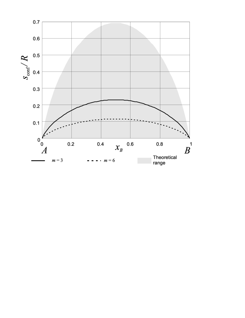
Figure 6: Molar configurational entropy of mixing given by the modified associate formalism in the limit of immiscible components.

Considering the limit of highly ordered solution, we assume also that the Gibbs free energy of associate with the composition $A_{2}B$ and with a particular spatial arrangement of particles approaches $-\infty$. The entropy curves for $m=3$ and $m=6$ given by the modified associate formalism in this case is presented in Fig. 7. In this case, the curves are also entirely located in the theoretically possible range.

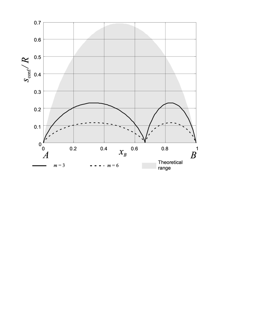
Figure 7: Molar configurational entropy of mixing given by the modified associate formalism in the limit of highly ordered solution.

2.4 Modified Quasichemical Model (1986)

In the modified quasichemical model, the molar configurational entropy of mixing is given by (see Eq. (10) in Ref. [6])

$$\begin{array}[]{l}s_{\text{conf}}=-R(x_{A}\ln(x_{A})+x_{B}\ln(x_{B}))\\ -R\left[n_{AA}\ln\left(\frac{x_{AA}}{y_{A}^{2}}\right)+n_{BB}\ln\left(\frac{x_{BB}}{y_{B}^{2}}\right)+n_{AB}\ln\left(\frac{x_{AB}}{2y_{A}y_{B}}\right)\right].\end{array}$$ (5)

Here, $x_{A}$ and $x_{B}$ are the molar fractions of the components $A$ and $B$; $n_{ij}$ and $x_{ij}$ ($i,j=A,B$) are the mole number and the molar fraction of $(i-j)$-pairs, respecively. The coordination-equivalent fractions $y_{A}$ and $y_{B}$ are defined as (see Eq. (6) in Ref. [6])

$$\begin{array}[]{ll}y_{A}&={Z_{A}n_{A}}/({Z_{A}n_{A}+Z_{B}n_{B}})\\ y_{B}&={Z_{B}n_{B}}/({Z_{A}n_{A}+Z_{B}n_{B}})~{},\end{array}$$ (6)

where $Z_{A}$ and $Z_{B}$ are the coordination numbers of the solution components $A$ and $B$, respectively. As demonstrated by Pelton and Blander [5] for constant coordination numbers and by Pelton et al. [6] for variable coordination numbers, the modified quasichemical model correctly reduces to the ideal solution model, when the Gibbs free energy change on forming $(A-B)$-pairs $\Delta g_{AB}$ equals to zero.

In the framework of MQM(1986) (the modified quasichemical model after Pelton and Blander [5]), the coordination numbers are assumed to be constant and are selected to set the composition of maximum ordering $x_{B}^{*}$ and to satisfy the conditions $s_{\text{conf}}=0$ at $x_{B}^{*}$ when $\Delta g_{AB}\rightarrow-\infty$. This results in (see also Eqs. (30) and (31) in Ref. [5])

$$\begin{array}[]{ll}Z_{B}&=-(x_{B}^{*}\ln(x_{B}^{*})+(1-x_{B}^{*})\ln(1-x_{B}^{*}))/(x_{B}^{*}\ln(2))\\ Z_{A}&=Z_{B}x_{B}^{*}/(1-x_{B}^{*}).\end{array}$$ (7)

Similar to the examples described above, consider one mole of binary solution $A-B$ and assume that $x_{B}^{*}=1/3$. In this case, $Z_{B}=2.75489$ and $Z_{A}=1.37744$. In the limit of immiscible components, $\Delta g_{AB}\rightarrow+\infty$. The molar configurational entropy of mixing given by the curves given by MQM(1986) in this case is presented in Fig. 8. As shown in this figure, MQM(1986) gives paradoxical, negative values of the configurational entropy of mixing for $0<x_{B}<1/3$.

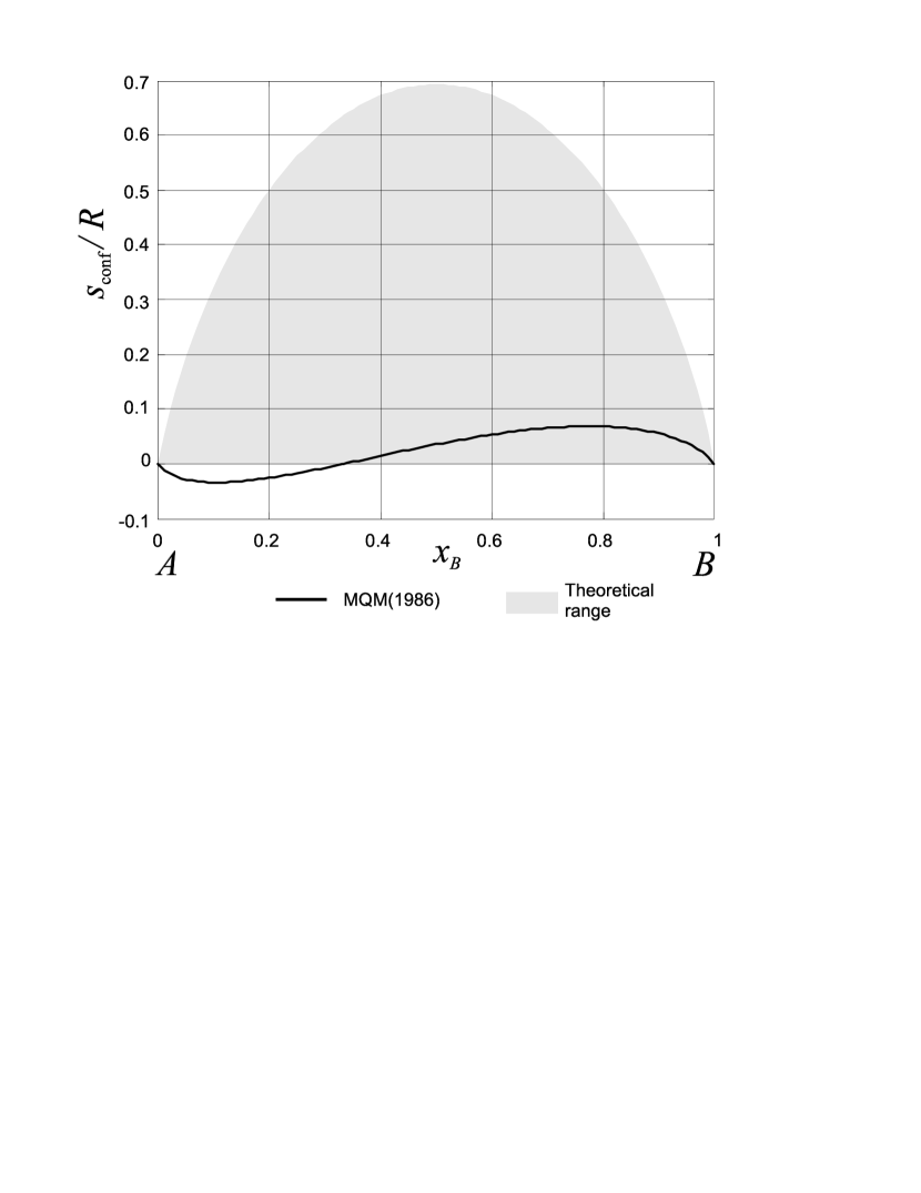
Figure 8: Molar configurational entropy of mixing given by the modified quasichemical model (1986) in the limit of immiscible components.

Now consider the limit of highly ordered liquid, that is, $\Delta g_{AB}\rightarrow-\infty$. Fig. 9 shows the entropy curve given by MQM(1986) in this case. As seen from Fig. 9, the curve is entirely located in the theoretically possible range.

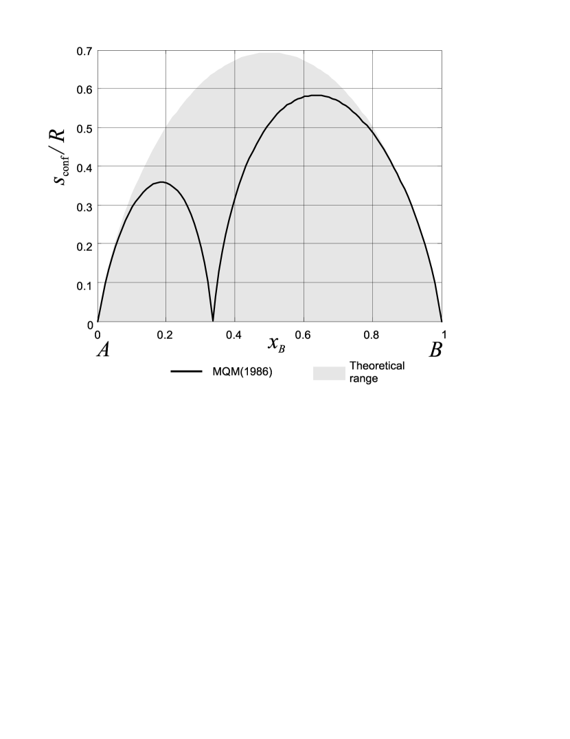
Figure 9: Molar configurational entropy of mixing given by the modified quasichemical model (1986) in the limit of highly ordered solution.

2.5 Modified Quasichemical Model (2000)

In the framework of MQM(2000) (the modified quasichemical model after Pelton et al. [6]), the configurational numbers are assumed to be composition-dependant. The following equations for the coordination numbers have been suggested (see Eqs. (19) and (20) in Ref. [6]):

$$\begin{array}[]{ll}\frac{1}{Z_{A}}&=\frac{1}{Z^{A}_{AA}}\frac{2n_{AA}}{2n_{AA}+n_{AB}}+\frac{1}{Z^{A}_{AB}}\frac{n_{AB}}{2n_{AA}+n_{AB}}\vspace{.2 cm}\\ \frac{1}{Z_{B}}&=\frac{1}{Z^{B}_{BB}}\frac{2n_{BB}}{2n_{BB}+n_{AB}}+\frac{1}{Z^{B}_{BA}}\frac{n_{AB}}{2n_{BB}+n_{AB}}~{}.\end{array}$$ (8)

Consider the limit of immiscible components ($\Delta g_{AB}\rightarrow+\infty$), assuming that the constants $Z^{A}_{AA}$, $Z^{B}_{BB}$, $Z^{A}_{AB}$ and $Z^{B}_{BA}$ are chosen as suggested by Pelton et al. [6], namely:

$$Z^{A}_{AA}=Z^{B}_{BB}=Z^{B}_{BA}=6;~{}~{}Z^{A}_{AB}=3~{}.$$ (9)

Fig. 10 demonstrates that MQM(2000) gives paradoxical values of the configurational entropy of mixing for the entire compositional range in the limit of of immiscible components.

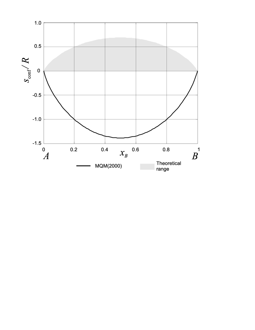
Figure 10: Molar configurational entropy of mixing given by the modified quasichemical model (2000) in the limit of immiscible components.

Now consider the limit of highly ordered solution, that is, $\Delta g_{AB}\rightarrow-\infty$. The entropy curve given by MQM(2000) in this case is presented in Fig. 11. As seen form this figure, MQM(2000) gives negative values of the configurational entropy of mixing in the vicinity of the composition of maximum ordering.

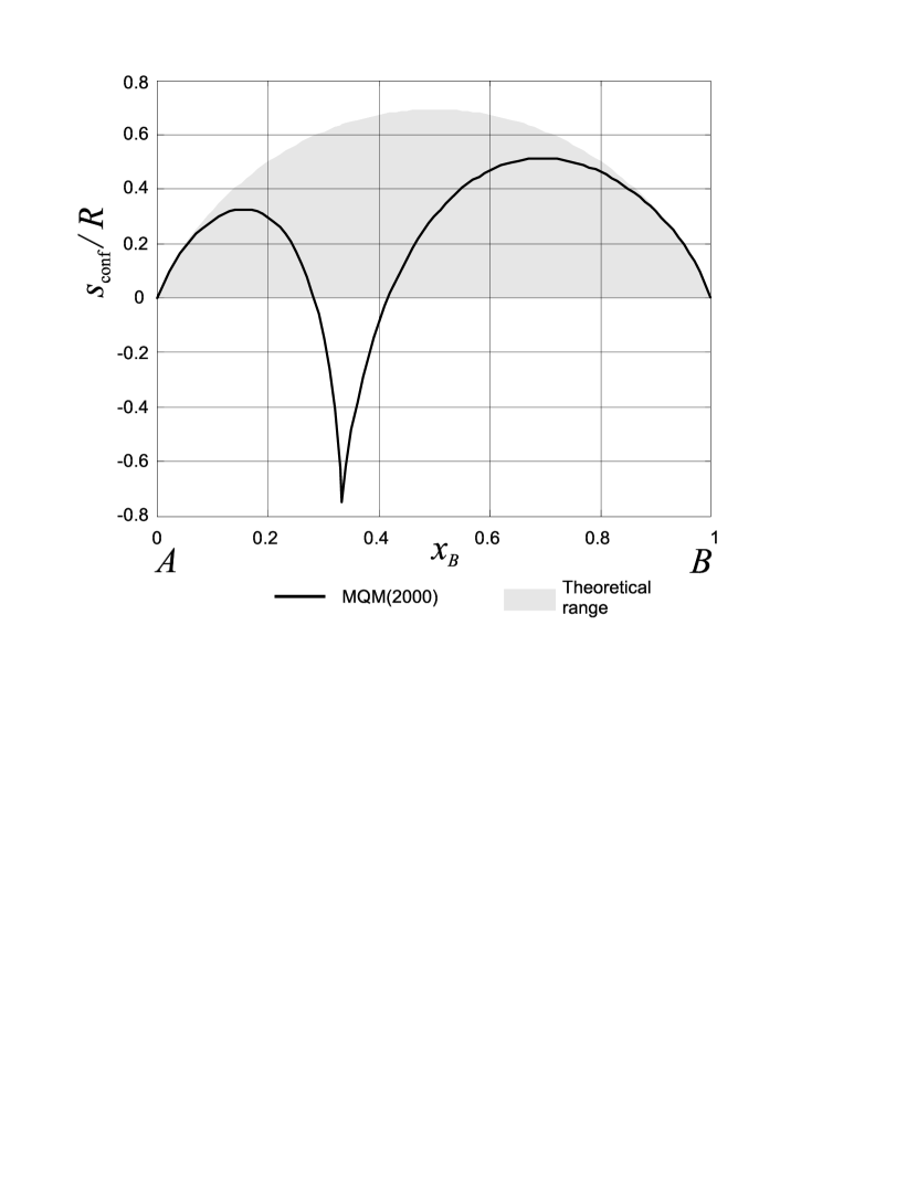
Figure 11: Molar configurational entropy of mixing given by the modified quasichemical model (2000) in the limit of highly ordered solution.

2.6 Classical Quasichemical Model

It is important to note that the classical quasichemical model of Fowler and Guggenheim [4] (with $Z_{A}=Z_{B}=1/2$) correctly reduces to the ideal solution model when $\Delta g_{AB}=0$. In the limit of immiscible components, the configurational entropy of mixing given by this model correctly reduces to the theoretically expected curve ($s_{\text{conf}}\equiv 0$). In all other cases, the classical quasichemical model gives values of the configurational entropy of mixing which are within the theoretically possible range. The applicability of the classical quasichemical model, however, is limited to those chemical solutions, in which maximum ordering occurs at the composition $x_{B}=1/2$.

2.7 Summary

The classical associate model results in paradoxically large values of the configurational entropy in the limit of ideal solution, while giving theoretically possible values of the configurational entropy of mixing in other two limits. The associate species model can give paradoxically large values in the limit of ideal solution and in the limit of highly ordered solution.

The modified quasichemical model after Pelton and Blander [5] results in paradoxically small, negative values of the configurational entropy in the limit of immiscible components. The modified quasichemical model after Pelton et al. [6] gives paradoxically small, negative values in the limit of immiscible components and in the limit of highly ordered solution.

The modified associate formalism [1] and the classical quasichemical model [4] give theoretically possible values of the configurational entropy in all considered limits. The classical quasichemical model also correctly reduces to the theoretically expected curve in the limit of immiscible components. The applicability of the classical quasichemical model, however, is limited.

3 Dilute Solutions

Pelton et al. [6] considered binary solution, in which maximum ordering occurs at the composition $x_{B}=1/3$ in the limit of highly ordered solution (Gibbs free energy change on forming $(A-B)$-pairs approaches $-\infty$). It was demonstrated that, in the framework of the modified quasichemical model, chemical activity $a_{B}$ of the component $B$ in the varies in the vicinity of $x_{A}=0$ as ($1-x_{A}$) even in this limiting case.

Similar solution has also been considered in Ref. [1] in the framework of the modified associate formalism. As demonstrated, chemical activity $a_{B}$ varies as ($1-x_{A}$) only for finite values of $\Delta g_{2,1}$ and $\Delta g_{1,2}$. Here, $\Delta g_{2,1}$ and $\Delta g_{1,2}$ are the molar Gibbs free energy changes on forming $A_{2}B$-associates and $AB_{2}$-associates, respectively. In the limit of highly ordered solution ($\Delta g_{2,1}\rightarrow-\infty$), $a_{B}$ varies as ($1-x_{A}/2$). Note also that the interval in the vicinity of $x_{A}=0$, in which $a_{B}$ can be approximated as ($1-x_{A}$), decreases with the decrease in $\Delta g_{2,1}$. This should be taken into consideration, when the modified associate formalism is used for modelling dilute solutions.

Now consider the solution discussed in in Ref. [1] in the framework of the associate species model. That is, we consider the associate species $A_{q}$, $B_{q}$, $A_{2q/3}B_{q/3}$ and $A_{q/3}B_{2q/3}$ of the size $q$. In this case, chemical activity $a_{B}$ is given by

$$a_{B}=x_{B_{q}}^{1/q}~{},$$ (10)

where $x_{B_{q}}$ is the molar fraction of the species $B_{q}$. Eq. (28) in Ref. [1] reads

$$\frac{da_{B}}{dx_{A}}=\frac{1}{q}x_{B_{q}}^{1/q-1}\left(\frac{dx_{A}}{dx_{B_{q}}}\right)^{-1}~{}.$$ (11)

Using the technique described in Section 6 of the previous paper [1], one verifies that

$$\begin{array}[]{ll}\frac{dx_{A}}{dx_{B_{q}}}&=-1-\frac{4}{9}\epsilon_{2}t-\frac{1}{9}\epsilon_{1}t^{2}\\ &+\frac{2}{9}\frac{\left(\epsilon_{2}+\epsilon_{1}t\right)\left(1+\frac{2}{3}\epsilon_{2}t+\frac{1}{3}\epsilon_{1}t^{2}\right)}{\left(t^{2}+\frac{1}{3}\epsilon_{2}+\frac{2}{3}\epsilon_{1}t\right)}\end{array}$$ (12)

Here, $t\equiv\left({x_{A_{q}}}/{x_{B_{q}}}\right)^{1/3}$, $\epsilon_{1}\equiv\exp\left(-{\Delta g_{A_{2q/3}B_{q/3}}}/{RT}\right)$ and $\epsilon_{2}\equiv$ $\exp\left(-{\Delta g_{A_{q/3}B_{2q/3}}}/{RT}\right)$, while $\Delta g_{A_{2q/3}B_{q/3}}$ and $\Delta g_{A_{q/3}B_{2q/3}}$ are the molar Gibbs free energies of formation of $A_{2q/3}B_{q/3}$-species and $A_{q/3}B_{2q/3}$-species, respecively.

Substituting Eq. (12) into Eq. (11) and taking the limit when $x_{A}\rightarrow 0$, one verifies that

$$\lim\limits_{x_{A}\rightarrow 0}(da_{B}/dx_{A})=-\frac{3}{q}~{}.$$ (13)

This demonstrates that, for any finite values of $\Delta g_{A_{2q/3}B_{q/3}}$ and $\Delta g_{A_{q/3}B_{2q/3}}$, chemical activity $a_{B}$ given by the associate species model varies as ($1-x_{A}$) only when $q=3$. In the limit of highly ordered solution ($\Delta g_{A_{2q/3}B_{q/3}}\rightarrow-\infty$), $a_{B}$ varies as ($1-\frac{3}{2q}x_{A}$) in the vicinity of $x_{A}=0$.

It is also important to note that, in the framework of the associate species model, one can consider the species $A_{q}$, $B_{q}$ and $A_{2q/3}B_{q/3}$ only, since the set of species to be considered is determined by a modeller. Formally setting $\Delta g_{A_{q/3}B_{2q/3}}=+\infty$, Eq. (12) reduces to

$$\frac{dx_{A}}{dx_{B_{q}}}=-1-\frac{1}{9}\epsilon_{1}t^{2}+\frac{2}{9}\frac{\epsilon_{1}t\left(1+\frac{1}{3}\epsilon_{1}t^{2}\right)}{\left(t^{2}+\frac{2}{3}\epsilon_{1}t\right)}~{}.$$ (14)

Substitution of Eq. (14) into Eq. (11) and taking the limit when $x_{A}\rightarrow 0$ gives

$$\lim\limits_{x_{A}\rightarrow 0}(da_{B}/dx_{A})=-\frac{3}{2q}~{}.$$ (15)

In this case, $a_{B}$ varies in the vicinity of $x_{A}=0$ as ($1-\frac{3}{2q}x_{A}$) for any value of $\Delta g_{A_{2q/3}B_{q/3}}$.

The examples presented above indicate that the set of associate species and the size of species should be carefully selected, when the associate species model is applied for dilute solutions.

4 Setting the Composition of Maximum Ordering

Modelling of multicomponent systems requires a provision for setting the composition of maximum ordering so as to comply with the experimental data for each sub-system (binary, ternary, quaternary and so on) individually. Associate-type models allow to do this in a straightforward way by including in each sub-system the associates, which composition coincides with that of maximum ordering in a particular sub-system. In the case of the classical associate model or the associate species model, a modeller can arbitrarily include the required associates or the associate species. In the case of the modified associate formalism, in which the compositions of associates are defined by their size, one should select the adequately large size of associates to include the required compositions.

In contrast to associate-type models, there are no provisions for setting the composition of maximum ordering for each ternary, quaternary and so on sub-systems individually neither in the framework of MQM(1986) nor in the framework of MQM(2000). Furthermore, the composition of maximum ordering can not be set independently even for binary sub-systems in the framework of MQM(1986). To overcome this disadvantage for binary sub-systems, Pelton et al. [6] suggested to use variable coordination numbers given by Eqs. (8). This modification, however, leads to mathematical and thermodynamical inconsistencies of MQM(2000). These inconsistencies are described immediately below.

Consider the case, in which the coordination numbers are given by Eqs. (8) and the constants $Z^{A}_{AA}$, $Z^{B}_{BB}$, $Z^{A}_{AB}$ and $Z^{B}_{BA}$ are given by Eqs. (9). Firstly, as demonstrated in Ref. [8], the total mole number of pairs $n_{\text{tp}}$ depends on the extent of the quasichemical reaction (Eq. (1) in Ref. [6]). More precisely, $n_{\text{tp}}$ decreases by $1/2$ mole per each mole of $(A-B)$ pairs formed. This result contradicts to the equation of the quasichemical reaction (see Eq. (1) in Ref. [6]), which underlies the quasichemical model. According to Eq. (1) in Ref. [6], $n_{\text{tp}}$ does not change in the quasichemical reaction. Secondly, when the coordination numbers $Z_{A}$ and $Z_{B}$ vary with $n_{AB}$, the expression for the Gibbs free energy of the solution given by Eq. (9) in Ref. [6]) is in error. Using Eqs. (1-3,19,20) in Ref. [6], one verifies that the correct expression in this case is

$$G=\frac{Z_{A}}{Z^{A}_{AA}}n_{A}g_{A}^{\circ}+\frac{Z_{B}}{Z^{B}_{BB}}n_{B}g_{B}^{\circ}-T\Delta S^{\text{config}}+\frac{n_{AB}}{2}\Delta g_{AB}~{}.$$ (16)

Here, all the notations have the same meaning as in Ref. [6].

5 Conclusions

The modified associate formalism has been compared with similar models. As demonstrated, the formalism gives theoretically possible values of the configurational entropy in all considered limits. Being an associate-type model, the formalism allows to set the composition of maximum ordering for each sub-system of a multicomponent system individually. The corrected Gibbs free energy equation of the quasichemical model is also presented.

References

- [1] D. N. Saulov, I. G. Vladimirov, A. Y. Klimenko, Modified associate formalism without entropy paradox Part I: Model Description, Submitted to Journal of Alloys and Compounds.
- [2] I. Prigogine, R. Defay, Chemical Thermodynamics, Longmans, Green and Co., 1954.
- [3] T. M. Besmann, K. E. Spear, Thermochemical modeling of oxide glasses, Journal of the American Ceramic Society 85 (12) (2002) 2887–2894.
- [4] R. H. Fowler, E. A. Guggenheim, Statistical Thermodynamics, Cambridge University Press, 1939.
- [5] A. D. Pelton, M. Blander, Thermodynamic analysis of ordered liquid solutions by a modified quasichemical approach - application to silicate slags, Metallurgical Transactions B: Process Metallurgy 17B (1986) 805–815.
- [6] A. D. Pelton, S. A. Degterov, G. Eriksson, C. Robelin, Y. Dessureault, The modified quasichemical model I - Binary solution, Metallurgical and Materials Transactions B: Process Metallurgy and Materials Processing Science 31B (2000) 651–659.
- [7] R. Lück, U. Gerling, B. Predel, An entropy paradox of the association model, Zeitschrift fur Metallkunde 80 (1989) 270–275.
- [8] D. Saulov, Shortcomings of the recent modifications of the quasichemical solution model, Calphad - Computer Coupling of Phase Diagrams and Thermochemistry 31 (2007) 390–395.