Modified Associate Formalism without Entropy Paradox:
Part I. Model Description

Abstract

A Modified Associate Formalism is proposed for thermodynamic modelling of solution phases. The approach is free from the entropy paradox described by Lück et al. (Z. Metallkd. 80 (1989) pp. 270–275). The model is considered in its general form for an arbitrary number of solution components and an arbitrary size of associates. Asymptotic behaviour of chemical activities of solution components in binary dilute solutions is also investigated.

, ,

1 Introduction

The associate model in its various modifications has been successfully used for modelling solution phases of metallurgical and chemical engineering interest [1, 2, 3, 4, 5, 6, 7]. Besmann and Spear [3], for example, utilised the modified associated species model for glasses used in nuclear waste disposal. Recently, Yazhenskikh et al. [5, 6, 7] have successfully applied the associate species model to model melting behaviour of coal ashes which is an important problem in coal gasification technologies. Good agreement between model predictions and available experimental data was reported.

According to the classical associate model described by Prigogine and Defay [8], the strong interactions result in the formation of stable configurations of mixing particles, the so-called association complexes or, briefly, associates. Those particles that are not involved in the formation of associates are called free particles or, interchangeably, monoparticles. The associated solution is then considered to be an ideal solution of monoparticles and different associates. For example, a binary associated solution of components $A$ and $B$, in which only $AB$-associates are formed, is considered to be a ternary ideal solution of the $A$-monoparticles, $B$-monoparticles and $AB$-associates.

The Gibbs free energy $G$ of the associated solution of $n_{A}$ moles of the solution component $A$ and $n_{B}$ moles of $B$ is then given by

$$G=n_{A_{1}}g_{A_{1}}+n_{B_{1}}g_{B_{1}}+n_{AB}g_{AB}-TS_{\text{conf}},$$ (1)

where the configurational entropy of mixing $S_{\text{conf}}$ is expressed as

$$S_{\text{conf}}=-R\left(n_{A_{1}}\ln x_{A_{1}}+n_{B_{1}}\ln x_{B_{1}}+n_{AB}\ln x_{AB}\right).$$ (2)

Here, $n_{A_{1}}$, $n_{B_{1}}$, $n_{AB}$ are the mole numbers and $g_{A_{1}}$, $g_{B_{1}}$, $g_{AB}$ are the molar Gibbs free energies of the $A$-monoparticles, $B$-monoparticles and $AB$-associates, respectively; $T$ is the absolute temperature and $R$ is the universal gas constant. The molar fractions $x_{A_{1}}$, $x_{B_{1}}$ and $x_{AB}$ are defined in a usual way. For example, $x_{A_{1}}=n_{A_{1}}/(n_{A_{1}}+n_{B_{1}}+n_{AB})$. The other molar fractions are defined similarly.

The equilibrium values of the mole numbers $n_{A_{1}}$, $n_{B_{1}}$ and $n_{AB}$ are determined by minimising the Gibbs free energy $G$ given by Eq. (1), subject to the mass balance constraints

$$\begin{array}[]{l}n_{A}=n_{A_{1}}+n_{AB},\\ n_{B}=n_{B_{1}}+n_{AB}.\end{array}$$ (3)

The adjustable parameter of the model is the molar Gibbs free energy $\Delta g_{AB}$ of the reaction

$$A+B\rightleftarrows AB.$$ (4)

Besmann and Spear [3] considered an ideal mixture of associate species (instead of monoparticles and associates). The stoichiometry of the associate species was specified so that all the species contain two non-oxygen atoms per formula unit. In this approach, contributions of different species to the configurational entropy of mixing are equally weighted.

Lück et al. [9] described a remarkable feature of the configurational entropy of mixing given by Eq. (2). This feature was referred to as an entropy paradox and is briefly described in the next section.

2 Entropy paradox

Lück et al. considered the high temperature limit for the associated solution. The temperature $T$ is assumed to be so high that the entropy term plays a dominant role in the Gibbs free energy of the solution and the enthalpy changes on forming different associates can be neglected. The configurational entropy of mixing given by Eq. (2) in the high temperature limit is higher than that used in the regular solution model (the entropy of ideal mixing of the solution components). For example, the configurational entropy of mixing of the associated solution in which only the ${AB}$-associates are formed is compared with the ideal entropy of mixing in Fig. 1.

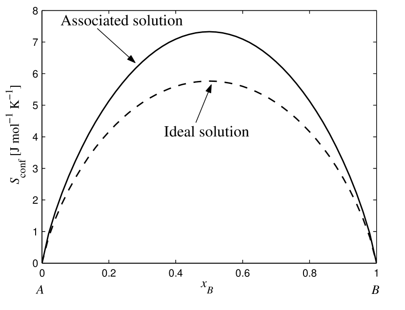
Figure 1: The configurational entropy of mixing for the associated solution, in which only the ${AB}$-associates are formed, in the high temperature limit compared with the ideal entropy of mixing.

At the same time, the formation of associates models short range ordering in the solution. As pointed out by Lück et al. [9], it is a paradoxical result that the configurational entropy, which is a measure of disorder, appears to be higher in a solution with ordering than in a completely disordered solution.

Another interpretation of this entropy paradox was described by Pelton et al. [10]. Consider the binary associated solution where only ${AB}$-associates are formed and assume that there are no Gibbs free energy changes on forming ${AB}$-associates from monoparticles, so that $\Delta g_{AB}=0$. In this case, the configurational entropy of mixing of the solution should be equal to that of an ideal solution, since no interactions between mixing particles are assumed. Eq. (2) however, leads to higher values for the configurational entropy of mixing that reduces to the ideal configurational entropy of mixing only when $\Delta g_{AB}=+\infty$; see also Fig. 1. The overestimation of the configurational entropy can result in either underestimation of the non-configurational entropy or overestimation of the enthalpy of mixing or both. This, in tern, can undermine the predictive capabilities of the model.

As pointed out by Lück et al. [9] and later by Pelton et al. [10], the expression for the configurational entropy of mixing used in the quasichemical model does reduce to the ideal configurational entropy of mixing when $\Delta g_{AB}=0$. In the next section, we propose the Modified Associate Formalism which is free of the entropy paradox. The paradox is resolved by distinguishing between all possible spatial arrangements of particles in an associate that have not been taken into account in previous associate models.

3 Model assumptions

The model proposed in this paper is based on the following assumptions.

1. Similarly to the classical associate model [8], we assume that interactions between mixing particles result in the formation of associates which are in a stable dynamic equilibrium with each other. The associates of the model are understood as a tool for modelling short-range interactions between mixing particles. The associates of the model, however, may represent real associated complexes present in solution phases.

2. We assume that the associates do not interact with each other and are uniformly distributed (ideally mixed) over a lattice. Equivalently, the occupancies of the sites of the associate lattice are stochastically independent and have identical probability distributions.

3. In contrast to the classical model, all pure solution components and the chemical solution of these components are treated in a unified way. More precisely, we assume that the solution and all its components consist of noninteracting associates of the same size, so that the associates are composed of the same number of particles. In this approach, the contributions of different associates to the configurational entropy of mixing are equally weighted.

4. Following the convention (see, for example, Ref. [11] for more details), we also assume that particles of the same type are indistinguishable, while particles of different types and particle sites within an associate are distinguishable.

4 Model description

For simplicity of exposition, we exemplify the model by considering a binary solution $A-B$ where the associates are composed of three particles. Let $n_{A}$ and $n_{B}$ be the mole numbers of $A$ and $B$ particles in the solution. Since, by assumption 4) above, the particle sites within an associate are distinguishable, we also assume that they are numbered. If the 1st and 2nd sites in an associate are both occupied by $A$-particles, while the 3rd one is occupied by a $B$-particle, such an associate is said to be of type $[AAB]$. Other types of associates are defined similarly. Thus, in the solution considered, there are $2^{3}=8$ different types of associates, $[AAA]$, $[BAA]$, $[ABA]$, $[AAB]$, $[BBA]$, $[BAB]$, $[ABB]$, $[BBB]$. It is important to note that all these types should be taken into account in calculating the configurational entropy.

Let $n_{[ijk]}$ be the mole number of $[ijk]$-associates, where the triplet of symbolic indices $i,j,k=A,B$ specify the associate type. Then the mass balance constraints take the form

$$\begin{array}[]{lcl}n_{A}&=&3n_{[AAA]}\\ &+&2(n_{[BAA]}+n_{[ABA]}+n_{[AAB]})\\ &+&n_{[BBA]}+n_{[BAB]}+n_{[ABB]},\\ n_{B}&=&3n_{[BBB]}\\ &+&2(n_{[ABB]}+n_{[BAB]}+n_{[BBA]})\\ &+&n_{[AAB]}+n_{[ABA]}+n_{[BAA]}.\end{array}$$ (5)

By a standard combinatorial argument, the number of available microstates $\Omega$ is

$$\Omega=\frac{\left(N_{\circ}\sum\limits_{i,j,k={A,B}}n_{[ijk]}\right)!}{\prod\limits_{i,j,k={A,B}}\left(N_{\circ}\,n_{[ijk]}\right)!},$$ (6)

where $N_{\circ}$ is the Avogadro number. Under assumption 2) of ideal mixing of associates, the configurational entropy of mixing $S_{\text{conf}}$ is

$$S_{\text{conf}}=k_{\text{B}}\ln\Omega~{},$$ (7)

where $k_{\text{B}}$ is Boltzmann’s constant. Applying the Stirling formula to Eqs. (6) and (7),

$$S_{\text{conf}}=-R\sum\limits_{i,j,k={A,B}}n_{[ijk]}\ln x_{[ijk]},$$ (8)

where

$$x_{[ijk]}=\frac{n_{[ijk]}}{\sum\limits_{i^{\prime},j^{\prime},k^{\prime}=A,B}\ n_{[i^{\prime}j^{\prime}k^{\prime}]}}$$

is the molar fraction of the $[ijk]$-associates. Therefore, the Gibbs free energy of the solution is given by

$$G=\sum\limits_{i,j,k={A,B}}n_{[ijk]}\left(g_{[ijk]}+RT\ln x_{[ijk]}\right),$$ (9)

where $g_{[ijk]}$ is the molar Gibbs free energy of $[ijk]$-associates. In one mole of pure solution component $A$ there are $1/3$ moles of $[AAA]$-associates. Hence, $g_{[AAA]}=3g_{A}$, where $g_{A}$ is the molar Gibbs free energy of the pure solution component $A$. Similarly, $g_{[BBB]}=3g_{B}$, where $g_{B}$ is the molar Gibbs free energy of the pure solution component $B$.

The associates, which consist of both $A$ and $B$ particles, will be referred to as mixed associates. For the binary solution considered, there are $8-2=6$ types of mixed associates. Their molar Gibbs free energies $g_{[ijk]}$, with $[ijk]\neq[AAA],[BBB]$, are adjustable parameters of the model. These parameters can depend on the temperature $T$ as

$$g_{[ijk]}=h_{[ijk]}-Ts_{[ijk]},$$ (10)

where $h_{[ijk]}$ and $s_{[ijk]}$ are the molar enthalpy and entropy of ${[ijk]}$-associates, respectively. Alternatively, as adjustable parameters of the model, one can employ the Gibbs free energies of the reactions of forming mixed associates from pure $[AAA]$ and $[BBB]$-associates. For example, instead of $g_{[AAB]}$, the Gibbs free energy $\Delta g_{[AAB]}$ of the following reaction can be used,

$$\frac{2}{3}[AAA]+\frac{1}{3}[BBB]\rightleftarrows[AAB],$$ (11)

so that

$$\Delta g_{[AAB]}=g_{[AAB]}-\frac{2}{3}g_{[AAA]}-\frac{1}{3}g_{[BBB]}.$$ (12)

The other Gibbs free energies $\Delta g_{[ijk]}$ are defined similarly.

Note that Eqs. (5) define $n_{[AAA]}$ and $n_{[BBB]}$ as linear functions of the mole numbers of the solution components $n_{A}$ and $n_{B}$ and of the mole numbers $n_{[ijk]}$ of the mixed associate types with $[ijk]\neq[AAA],[BBB]$. The mole numbers of the latter associates, which consist of both $A$ and $B$ particles, are the internal variables of the model. These are determined by minimising the Gibbs free energy of the solution at constant $n_{A}$ and $n_{B}$, subject to the mass balance constrains of Eqs. (5). The equilibrium values of $n_{[ijk]}$, with $[ijk]\neq{[AAA],[BBB]}$, are found from

$$\left(\frac{\partial G}{\partial n_{[ijk]}}\right)_{n_{A},\,n_{B},\,n_{[i^{\prime}j^{\prime}k^{\prime}]}}=0,$$ (13)

where the derivative in $n_{[ijk]}$ is calculated for fixed $n_{A}$, $n_{B}$ and fixed five variables $n_{[i^{\prime}j^{\prime}k^{\prime}]}$, with $[i^{\prime}j^{\prime}k^{\prime}]\neq[ijk],[AAA],[BBB]$. By the chain rule, Eq. (13) reads

$$\frac{\partial G}{\partial n_{[AAA]}}\frac{\partial n_{[AAA]}}{\partial n_{[ijk]}}+\frac{\partial G}{\partial n_{[BBB]}}\frac{\partial n_{[BBB]}}{\partial n_{[ijk]}}+\frac{\partial G}{\partial n_{[ijk]}}=0.$$ (14)

Therefore, combining the last equation with Eqs. (5) and (9) gives

$$\frac{n_{[ijk]}}{(n_{[AAA]})^{\alpha_{[ijk]}/3}(n_{[BBB]})^{\beta_{[ijk]}/3}}=\exp\left(-\frac{\Delta g_{[AAB]}}{RT}\right).$$ (15)

Here, $\alpha_{[ijk]}$ and $\beta_{[ijk]}$ stand for the numbers of $A$ and $B$ particles in the $[ijk]$-associate, respectively. For example, $\alpha_{[AAB]}=2$ and $\beta_{[AAB]}=1$.

Recall that Eqs. (5) define $n_{[AAA]}$ as a linear function of $n_{A}$ and $n_{[ijk]}$’s, and $n_{[BBB]}$ as a linear function of $n_{B}$ and $n_{[ijk]}$’s, where $[ijk]\neq[AAA],[BBB]$. The chemical potential $\mu_{A}$ of the solution component $A$ is calculated as follows

$$\begin{array}[]{lll}\mu_{A}&=&\left(\frac{\partial G}{\partial n_{A}}\right)_{n_{B}}\\ &=&\sum\limits_{[ijk]}{\frac{\partial G}{\partial n_{[ijk]}}\frac{\partial n_{[ijk]}}{\partial n_{A}}}\\ &+&\frac{\partial G}{\partial n_{[AAA]}}\left(\frac{\partial n_{[AAA]}}{\partial n_{A}}+\sum\limits_{[ijk]}{\frac{\partial n_{[AAA]}}{\partial n_{[ijk]}}\frac{\partial n_{[ijk]}}{\partial n_{A}}}\right)\\ &+&\frac{\partial G}{\partial n_{[BBB]}}\left(\frac{\partial n_{[BBB]}}{\partial n_{A}}+\sum\limits_{[ijk]}{\frac{\partial n_{[BBB]}}{\partial n_{[ijk]}}\frac{\partial n_{[ijk]}}{\partial n_{A}}}\right)\\ &=&\frac{\partial G}{\partial n_{[AAA]}}\frac{\partial n_{[AAA]}}{\partial n_{A}}+\sum\limits_{[ijk]}\left(\frac{\partial G}{\partial n_{[AAA]}}\frac{\partial n_{[AAA]}}{\partial n_{[ijk]}}\right.\\ &&\left.+\frac{\partial G}{\partial n_{[BBB]}}\frac{\partial n_{[BBB]}}{\partial n_{[ijk]}}+\frac{\partial G}{\partial n_{[ijk]}}\right)\frac{\partial n_{[ijk]}}{\partial n_{A}}.\end{array}$$ (16)

Here, the sums are taken over $i,j,k={A,B}$ such that $[ijk]\neq[AAA],[BBB]$. Using Eqs. (9) and (14), one verifies that

$$\mu_{A}=\frac{\partial G}{\partial n_{[AAA]}}\frac{\partial n_{[AAA]}}{\partial n_{A}}=g_{A}+\frac{1}{3}RT\ln x_{[AAA]}.$$ (17)

The chemical potential $\mu_{B}$ of the solution component $B$ is calculated in a similar way.

Note that $[AAB]$, $[ABA]$ and $[BAA]$ associates differ in the spatial arrangement of the constituent particles, though they have the same “chemical composition” $A_{2}B$. The same distinction holds for $[BBA]$, $[BAB]$ and $[ABB]$ associates of common composition $AB_{2}$. Let us assume, for a moment, that only one spatial arrangement of associates is allowed for each composition, while the other arrangements are prohibited energetically, for example, $g_{[BAA]}=g_{[ABA]}=+\infty$ and $g_{[BAB]}=g_{[ABB]}=+\infty$. In this case, the proposed formalism reduces to the associate species model [3], in which associate species are composed of three particles.

Unlike previous modifications of the associate model, we take into account all possible spatial arrangements of particles in an associate. If two or more associates of different types are spatially symmetric to each other, then their molar Gibbs free energies are considered equal. For example, 2-particle associates $[AB]$ and $[BA]$ are symmetric and therefore are endowed with equal Gibbs energies $g_{[AB]}=g_{[BA]}$.

In more complex cases, however, Gibbs free energy levels are ascribed to associates depending on the spatial arrangement of particles in them, so that both energy splits and multiple levels may occur for associates of common chemical composition. For example, if particle sites in 3-particle associates are arranged linearly as shown in Fig. 2(a), then $g_{[AAB]}=g_{[BAA]}$ while $g_{[ABA]}$ can be different. Alternatively, if the particle sites are arranged as in Fig. 2(b), the three associate types are all symmetric to each other, and hence, $g_{[AAB]}=g_{[ABA]}=g_{[BAA]}$.

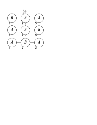
(a) Particle sites are arranged along a (horizontal) line. The associates $[BAA]$ and $[AAB]$ are mirror reflections of each other about axis $a$; they are not symmetric, however, to $[ABA]$.

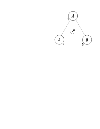
(b) Particle sites are arranged at the vertices of an equilateral triangle. All associates are symmetric to each other by rotation about axis $b$, perpendicular to the plane of the triangle.

Figure 2: Schematic views of different arrangements of particle sites.

Note that no assumptions on spatial arrangements of particle sites within an associate have been made so far in the framework of the proposed model. In general, it is impossible to determine in advance the number of energy levels and their multiplicities for the associates of a particular composition. Furthermore, such associates may have the same Gibbs free energy of formation, even if they are not spatially symmetric. As a reasonable initial approximation, all associates of a given composition can be endowed with the same Gibbs energy of formation. This assumption can be refined subsequently in the process of thermodynamic model optimisation for real chemical systems, if use of several energy levels appears to provide a better fit to experimental data.

For the rest of this section and also in Sections 5 and 6, we assume, for simplicity, that the molar Gibbs free energy of an associate type is completely specified by its chemical composition,

$$\begin{array}[]{l}\Delta g_{[AAB]}=\Delta g_{[ABA]}=\Delta g_{[BAA]}\equiv\Delta g_{2,1},\\ \Delta g_{[BBA]}=\Delta g_{[BAB]}=\Delta g_{[ABB]}\equiv\Delta g_{1,2}.\end{array}$$ (18)

Here, the subscript “2,1” signifies that the associate consists of two $A$-particles and one $B$-particle, with “1,2” and similar indices understood appropriately. More general case is considered in Section 7.

Using Eqs. (15) and (18),

$$\begin{array}[]{l}n_{[AAA]}\equiv n_{3,0},\\ n_{[AAB]}=n_{[ABA]}=n_{[BAA]}\equiv n_{2,1}/3,\\ n_{[BBA]}=n_{[BAB]}=n_{[ABB]}\equiv n_{1,2}/3,\\ n_{[BBB]}\equiv n_{0,3}.\end{array}$$ (19)

In terms of molar fractions, Eqs. (19) read

$$\begin{array}[]{l}x_{[AAA]}\equiv x_{3,0},\\ x_{[AAB]}=x_{[ABA]}=x_{[BAA]}\equiv x_{2,1}/3,\\ x_{[BBA]}=x_{[BAB]}=x_{[ABB]}\equiv x_{1,2}/3,\\ x_{[BBB]}\equiv x_{0,3}~{}.\end{array}$$ (20)

Substitution of Eqs. (19) and (20) into Eq. (9) gives

$$\begin{array}[]{lll}G&=&n_{3,0}g_{3,0}+n_{0,3}g_{0,3}+n_{2,1}g_{2,1}+n_{1,2}g_{1,2}\\ &+&RT\left(n_{3,0}\ln x_{3,0}+n_{0,3}\ln x_{0,3}\right)\\ &+&RT\left(n_{2,1}\ln\left(\frac{x_{2,1}}{3}\right)+n_{1,2}\ln\left(\frac{x_{1,2}}{3}\right)\right).\end{array}$$ (21)

The mass balance constraints of Eqs. (5) reduce to

$$\begin{array}[]{lll}n_{A}&=&3n_{3,0}+2n_{2,1}+n_{1,2},\\ n_{B}&=&3n_{0,3}+2n_{1,2}+n_{2,1}.\end{array}$$ (22)

The equilibrium values of the associate mole numbers are determined by

$$\begin{array}[]{l}\frac{n_{2,1}}{n_{3,0}^{2/3}n_{0,3}^{1/3}}=3\exp\left(-\frac{\Delta g_{2,1}}{RT}\right),\\ \frac{n_{1,2}}{n_{3,0}^{1/3}n_{0,3}^{2/3}}=3\exp\left(-\frac{\Delta g_{1,2}}{RT}\right).\end{array}$$ (23)

5 Case $\Delta g_{2,1}=0$ and $\Delta g_{1,2}=0$

Recalling Eq. (18), consider the situation where there are no Gibbs free energy changes of forming different associates, that is, $\Delta g_{2,1}=0$ and $\Delta g_{1,2}=0$. In this case, the $A$ and $B$ particle species mix ideally. The composition of a randomly selected triplet of particles follows the binomial distribution, well-known in probability theory; see, for example, Ref. [12]. More precisely, the probabilities of choosing an associate of particular compositions, or, equivalently, the molar fractions of appropriate associates, are

$$\begin{array}[]{ll}x_{3,0}&=x_{A}^{3},\\ x_{2,1}&=3x_{A}^{2}x_{B},\\ x_{1,2}&=3x_{A}x_{B}^{2},\\ x_{0,3}&=x_{B}^{3}.\end{array}$$ (24)

Here, $x_{A}$ and $x_{B}$ are the molar fractions of $A$ and $B$ particles. Since the total mole number of associates $n_{\text{tot}}$ is equal to $(n_{A}+n_{B})/3$, then the mole numbers of associates are given by

$$\begin{array}[]{lll}n_{3,0}&=&\frac{n_{A}^{3}}{3(n_{A}+n_{B})^{2}},\\ n_{2,1}&=&\frac{n_{A}^{2}n_{B}}{(n_{A}+n_{B})^{2}},\\ n_{1,2}&=&\frac{n_{A}n_{B}^{2}}{(n_{A}+n_{B})^{2}},\\ n_{0,3}&=&\frac{n_{B}^{3}}{3(n_{A}+n_{B})^{2}}.\end{array}$$ (25)

By direct inspection, the mole numbers given by Eqs. (25) satisfy Eqs. (22) and Eqs. (23) with $\Delta g_{2,1}=0$ and $\Delta g_{1,2}=0$. Since the Gibbs free energy $G$ given by Eq. (21) is a strictly convex function of the mole numbers of associates, then Eq. (23) has no other solution satisfying the mass balance.

Furthermore, if $\Delta g_{2,1}=0$ and $\Delta g_{1,2}=0$, then the molar Gibbs free energies of associates are given by

$$\begin{array}[]{ll}g_{3,0}&=3g_{A},\\ g_{2,1}&=2g_{A}+g_{B},\\ g_{1,2}&=g_{A}+2g_{B},\\ g_{0,3}&=3g_{B}.\end{array}$$ (26)

Finally, substitution of Eqs. (25) and (26) into Eq. (21) yields

$$G=n_{A}g_{A}+n_{B}g_{B}+RT\left(n_{A}\ln x_{A}+n_{B}\ln x_{B}\right).$$ (27)

Thus, the proposed model correctly reduces to the ideal solution model in the case where there are no interactions between mixing particles.

6 Dilute solutions

Pelton et al. [10] pointed out another interesting feature of the associate model that occurs in dilute solutions. They considered the associated solution of monoparticles $A$ and $B$ and associates $A_{2}B$. The highly ordered solution rich in component $B$ consists primarily of $B$-monoparticles and $A_{2}B$-associates. According to the authors, the chemical activity $a_{B}$ of the component $B$ behaves asymptotically as $(1-x_{A}/2)$ rather than $(1-x_{A})$ for small $x_{A}$. Thus, $\lim\limits_{x_{A}\rightarrow 0}(da_{B}/dx_{A})=-1/2$. Note, however, that this behaviour of $a_{B}$ is observed only in the limiting case $\Delta g_{2,1}=-\infty$. For any finite value, $\lim\limits_{x_{A}\rightarrow 0}(da_{B}/dx_{A})=-1$. We present the proof of this result for the model proposed in this paper. Using the presented technique, similar result can be established for the example considered by Pelton et al. [10].

As obtained in Section 4, $a_{B}=x_{0,3}^{1/3}$. The required derivative is then calculated as follows. First,

$$\frac{da_{B}}{dx_{A}}=\frac{1}{3}x_{0,3}^{-2/3}\frac{dx_{0,3}}{dx_{A}}=\frac{1}{3}x_{0,3}^{-2/3}\left(\frac{dx_{A}}{dx_{0,3}}\right)^{-1}.$$ (28)

Secondly, assuming $\Delta g_{2,1}$ and $\Delta g_{1,2}$ finite and denoting the right hand sides of Eqs. (LABEL:eq_equlibrium_conditions1) by

$$\epsilon_{2,1}\equiv 3\exp\left(-\frac{{\Delta g_{2,1}}}{RT}\right),\quad\epsilon_{1,2}\equiv 3\exp\left(-\frac{{\Delta g_{1,2}}}{RT}\right),$$ (29)

we obtain

$$\begin{array}[]{l}x_{2,1}=\epsilon_{2,1}{x_{3,0}^{2/3}x_{0,3}^{1/3}},\\ x_{1,2}=\epsilon_{1,2}{x_{3,0}^{1/3}x_{0,3}^{2/3}}.\end{array}$$ (30)

Substitution of Eqs. (30) into the mass balance constraints of Eqs. (22), with the latter written in terms of molar fractions, gives

$$1=x_{3,0}+x_{0,3}+\epsilon_{2,1}{x_{3,0}^{2/3}x_{0,3}^{1/3}}+\epsilon_{1,2}{x_{3,0}^{1/3}x_{0,3}^{2/3}},$$ (31)

$$1-x_{A}=x_{0,3}+\frac{1}{3}\epsilon_{2,1}{x_{3,0}^{2/3}x_{0,3}^{1/3}}+\frac{2}{3}\epsilon_{1,2}{x_{3,0}^{1/3}x_{0,3}^{2/3}}.$$ (32)

Now, Eq. (31) implicitly defines $x_{0,3}$ as a function of $x_{3,0}$, while Eq. (32) defines $x_{A}$ as a function of $x_{3,0}$ and $x_{0,3}$. Differentiating Eq. (31) gives

$$\frac{dx_{3,0}}{dx_{0,3}}=-\frac{1+\frac{2}{3}\epsilon_{1,2}t+\frac{1}{3}\epsilon_{2,1}t^{2}}{1+\frac{1}{3}\epsilon_{1,2}t^{-1}+\frac{2}{3}\epsilon_{2,1}t^{-2}},$$ (33)

where

$$t\equiv\left(\frac{x_{3,0}}{x_{0,3}}\right)^{1/3}~{}.$$ (34)

Differentiation of Eq. (32) with respect to $x_{0,3}$ and substitution of Eq. (34) into the resultant expression yields

$$\begin{array}[]{ll}\frac{dx_{A}}{dx_{0,3}}&=-1-\frac{4}{9}\epsilon_{1,2}t-\frac{1}{9}\epsilon_{2,1}t^{2}\\ &+\frac{2}{9}\frac{\left(\epsilon_{1,2}t^{-2}+\epsilon_{2,1}t^{-1}\right)\left(1+\frac{2}{3}\epsilon_{1,2}t+\frac{1}{3}\epsilon_{2,1}t^{2}\right)}{\left(1+\frac{1}{3}\epsilon_{1,2}t^{-2}+\frac{2}{3}\epsilon_{2,1}t^{-1}\right)}\\ &=-1-\frac{4}{9}\epsilon_{1,2}t-\frac{1}{9}\epsilon_{2,1}t^{2}\\ &+\frac{2}{9}\frac{\left(\epsilon_{1,2}+\epsilon_{2,1}t\right)\left(1+\frac{2}{3}\epsilon_{1,2}t+\frac{1}{3}\epsilon_{2,1}t^{2}\right)}{\left(t^{2}+\frac{1}{3}\epsilon_{1,2}+\frac{2}{3}\epsilon_{2,1}t\right)}.\end{array}$$ (35)

Note that $x_{0,3}\rightarrow 1$, $x_{3,0}\rightarrow 0$ and $t\rightarrow 0$ as $x_{A}\rightarrow 0$. Therefore, substituting Eq. (35) into Eq. (28) and taking the limit as $x_{A}\rightarrow 0$, one verifies that $\lim\limits_{x_{A}\rightarrow 0}(da_{B}/dx_{A})=-1$ for any finite values of $\Delta g_{2,1}$ and $\Delta g_{1,2}$.

Now consider the limiting case where $\Delta g_{2,1}\rightarrow-\infty$, while $\Delta g_{1,2}$ remains finite. Recalling Eqs. (29) and taking the limit in Eq. (35) give

$$\lim\limits_{\epsilon_{2,1}\rightarrow+\infty}\frac{dx_{A}}{dx_{0,3}}=-\frac{2}{3}-\frac{1}{6}\epsilon_{1,2}t-\frac{1}{6}t^{3}.$$ (36)

Finally, substituting Eq. (36) into Eq. (28) and taking the limit as $x_{A}\rightarrow 0$, we obtain $\lim\limits_{x_{A}\rightarrow 0}(da_{B}/dx_{A})=-1/2$ as $\Delta g_{2,1}\rightarrow-\infty$.

7 Model equations for arbitrary number of solution components and arbitrary size of associates

Consider an $r$-component solution $A_{1}-\ldots-A_{r}$ and assume that the components and the solution itself all consist of $m$-particle associates. There are $r^{m}$ distinguishable types of associates. Some of these types have the same compositions. Now consider an $m$-particle associate that consists of $k_{1},\ldots,k_{r}$ particles of types $A_{1},\ldots,A_{r}$, respectively. Thus, the composition of the associate is specified by the $r$-tuple of nonnegative integers $(k_{1},\dots,k_{r})$ satisfying $k_{1}+\ldots+k_{r}=m$. Omitting the dependence on $r$, the set of such tuplets, which represent all possible compositions of $m$-particle associates in the $r$-component solution, is denoted by ${\mathfrak{S}_{m}}$. Its cardinality, that is, the number ${N_{\text{comp}}}$ of different compositions is computed as

$$N_{\text{comp}}=\frac{(m+r-1)!}{m!(r-1)!}~{}.$$ (37)

Consider a pure solution component $A_{i}$. Its $m$-particle associates all have the composition

$$\sigma_{i}\equiv(\small{\underset{i-1}{\underbrace{0,\dots,0}}},m,\small{\underset{r-i}{\underbrace{0,\dots,0}}}).$$ (38)

The compositions $\sigma_{1},\ldots,\sigma_{r}$ and corresponding associate types are referred to as pure. The complementary set ${\mathfrak{S}_{m}}\setminus\{\sigma_{1},\ldots,\sigma_{r}\}$ of mixed compositions, containing two or more different particle species, is written briefly as $\mathfrak{S}^{\circ}_{m}$. Thus, $\mathfrak{S}^{\circ}_{m}$ is constituted by those $r$-tuples $(k_{1},\ldots,k_{r})$ from ${\mathfrak{S}_{m}}$ with at least two nonzero entries.

In one mole of the solution component $A_{i}$, there are $1/m$ moles of $m$-particle associates of composition $\sigma_{i}$. Thus, their molar Gibbs free energy $g_{\sigma_{i}}$ is

$$g_{\sigma_{i}}=mg_{i},$$ (39)

where $g_{i}$ is the molar Gibbs free energy of the solution component $A_{i}$.

In general, the total number $N_{k_{1},\ldots,k_{r}}$ of distinguishable types of associates which have the same composition ${k_{1},\ldots,k_{r}}$ is described by the multinomial coefficient

$$N_{k_{1},\ldots,k_{r}}=\frac{m!}{\prod\limits_{i=1}^{r}k_{i}!}.$$ (40)

We assume that all distinguishable types of the associates of composition $({k_{1},\ldots,k_{r}})$ are endowed with $J_{k_{1},\ldots,k_{r}}$ different values of the molar Gibbs free energy. Let $d_{k_{1},\ldots,k_{r}}^{[j]}$ be the number of the associate types at the $j$th energy level $g_{k_{1},\ldots,k_{r}}^{[j]}$, that is, the multiplicity of the level, so that

$$\sum\limits_{j=1}^{J_{k_{1},\ldots,k_{r}}}d_{k_{1},\ldots,k_{r}}^{[j]}=N_{k_{1},\ldots,k_{r}}.$$ (41)

All the $d_{k_{1},\ldots,k_{r}}^{[j]}$ associate types have the same molar Gibbs free energy of formation $\Delta g_{k_{1},\ldots,k_{r}}^{[j]}$ according to the reaction

$$\frac{k_{1}}{m}(A_{1})_{m}+\ldots+\frac{k_{r}}{m}(A_{r})_{m}\rightleftarrows\left((A_{1})_{k_{1}}\ldots(A_{r})_{k_{r}}\right)^{[j]}.$$ (42)

More precisely, the Gibbs free energy of the reaction is defined by

$$\Delta g_{k_{1},\ldots,k_{r}}^{[j]}=g_{k_{1},\ldots,k_{r}}^{[j]}-\frac{k_{1}}{m}g_{\sigma_{1}}-\ldots-\frac{k_{r}}{m}g_{\sigma_{r}}.$$ (43)

The molar Gibbs free energies $g_{k_{1},\ldots,k_{r}}^{[j]}$ of mixed associates of composition $({k_{1},\ldots,k_{r}})\in\mathfrak{S}^{\circ}_{m}$, or alternatively, the corresponding formation energies $\Delta g_{k_{1},\ldots,k_{r}}^{[j]}$ from Eq. (43) are adjustable parameters of the model.

Now let $n_{k_{1},\ldots,k_{r}}^{[j]}$ denote the mole number of the associates of composition $({k_{1},\ldots,k_{r}})$ at the $j$th energy level. The mass balance constraints then read

$$n_{i}=\sum\limits_{({k_{1},\ldots,k_{r}})\in{\mathfrak{S}_{m}}}k_{i}\sum\limits_{j=1}^{J_{k_{1},\ldots,k_{r}}}n_{k_{1},\ldots,k_{r}}^{[j]},\qquad i=1,\ldots,r,$$ (44)

where $n_{i}$ is the mole number of $A_{i}$ particles in the solution. One verifies that

$$\sum\limits_{i=1}^{r}n_{i}=m\sum\limits_{({k_{1},\ldots,k_{r}})\in{\mathfrak{S}_{m}}}\sum\limits_{j=1}^{J_{k_{1},\ldots,k_{r}}}n_{k_{1},\ldots,k_{r}}^{[j]}\equiv m\,n_{\text{tot}}.$$ (45)

Note that the total number of associates $n_{\text{tot}}$ is independent of composition of the solution since they are assumed to be of equal size. The Gibbs free energy of the solution is computed as

$$\begin{array}[]{lcl}G&=&\sum\limits_{({k_{1},\ldots,k_{r}})\in{\mathfrak{S}_{m}}}\sum\limits_{j=1}^{J_{k_{1},\ldots,k_{r}}}n_{k_{1},\ldots,k_{r}}^{[j]}g_{k_{1},\ldots,k_{r}}^{[j]}\\ &+&RT\sum\limits_{({k_{1},\ldots,k_{r}})\in{\mathfrak{S}_{m}}}\sum\limits_{j=1}^{J_{k_{1},\ldots,k_{r}}}n_{k_{1},\ldots,k_{r}}^{[j]}\ln\left(\frac{x_{k_{1},\ldots,k_{r}}^{[j]}}{d_{k_{1},\ldots,k_{r}}^{[j]}}\right),\end{array}$$ (46)

where

$$x_{k_{1},\ldots,k_{r}}^{[j]}=\frac{n_{k_{1},\ldots,k_{r}}^{[j]}}{n_{\text{tot}}}$$ (47)

is the molar fraction of an appropriate associate type.

Eqs. (44) define $n_{\sigma_{i}}$ as a linear function of the mole number $n_{i}$ of the solution component $A_{i}$ and of the mole numbers of the mixed associates $n_{k_{1},\ldots,k_{r}}^{[j]}$, where $({k_{1},\ldots,k_{r}})\in\mathfrak{S}^{\circ}_{m}$. The equilibrium values of $n_{k_{1},\ldots,k_{r}}^{[j]}$, which are internal variables of the model, are determined by minimising the Gibbs free energy of the solution at constant $n_{1},\ldots,n_{r}$, subject to the mass balance constraints of Eqs. (44). The minimum is found by setting

$$\left(\frac{\partial G}{\partial n_{k_{1},\ldots,k_{r}}^{[j]}}\right)_{n_{1},\ldots,n_{r}}=0$$ (48)

for all $({k_{1},\ldots,k_{r}})\in\mathfrak{S}^{\circ}_{m}$ and for all ${[j]}=1,\dots,J_{k_{1},\ldots,k_{r}}$. Recalling that $n_{\sigma_{i}}$ are functions of $n_{k_{1},\ldots,k_{r}}^{[j]}$, where $({k_{1},\ldots,k_{r}})\in\mathfrak{S}^{\circ}_{m}$, and using the chain rule,

$$\frac{\partial G}{\partial n_{k_{1},\ldots,k_{r}}^{[j]}}+\sum\limits_{i=1}^{r}\frac{\partial G}{\partial n_{\sigma_{i}}}\frac{\partial n_{\sigma_{i}}}{\partial n_{k_{1},\ldots,k_{r}}^{[j]}}=0.$$ (49)

Substitution of Eqs. (44) and (46) into Eq. (49) gives

$$\frac{n_{k_{1},\ldots,k_{r}}^{[j]}}{\prod\limits_{i=1}^{r}(n_{\sigma_{i}})^{k_{i}/m}}=d_{k_{1},\ldots,k_{r}}^{[j]}\exp\left(-\frac{\Delta g_{k_{1},\ldots,k_{r}}^{[j]}}{RT}\right).$$ (50)

Using Eqs. (44), one verifies that $n_{\sigma_{i}}$ is a function of $n_{i}$ and of $n_{k_{1},\ldots,k_{r}}^{[j]}$, where $({k_{1},\ldots,k_{r}})\in\mathfrak{S}^{\circ}_{m}$. The chemical potential $\mu_{1}$ of the solution component $A_{1}$ can now be calculated as follows:

$$\!\!\begin{array}[]{lcl}\mu_{1}&=&\left(\frac{\partial G}{\partial n_{1}}\right)_{n_{2},\dots,n_{r}}\\ &=&\sum\limits_{({k_{1},\ldots,k_{r}})\in\mathfrak{S}^{\circ}_{m}}\sum\limits_{j=1}^{J_{k_{1},\ldots,k_{r}}}\frac{\partial G}{\partial n_{k_{1},\ldots,k_{r}}^{[j]}}\frac{\partial n_{k_{1},\ldots,k_{r}}^{[j]}}{\partial n_{1}}\\ &+&\sum\limits_{i=1}^{r}\frac{\partial G}{\partial n_{\sigma_{i}}}\left(\frac{\partial n_{\sigma_{i}}}{\partial n_{1}}+\sum\limits_{({k_{1},\ldots,k_{r}})\in\mathfrak{S}^{\circ}_{m}}\sum\limits_{j=1}^{J_{k_{1},\ldots,k_{r}}}\frac{\partial n_{\sigma_{i}}}{\partial n_{k_{1},\ldots,k_{r}}^{[j]}}\frac{\partial n_{k_{1},\ldots,k_{r}}^{[j]}}{\partial n_{1}}\right)\\ &=&\frac{\partial G}{\partial n_{\sigma_{1}}}\frac{\partial n_{\sigma_{1}}}{\partial n_{1}}+\sum\limits_{({k_{1},\ldots,k_{r}})\in\mathfrak{S}^{\circ}_{m}}\sum\limits_{j=1}^{J_{k_{1},\ldots,k_{r}}}\left(\frac{\partial G}{\partial n_{k_{1},\ldots,k_{r}}^{[j]}}\right.\\ &+&\left.\sum\limits_{i=1}^{r}\frac{\partial G}{\partial n_{\sigma_{i}}}\frac{\partial n_{\sigma_{i}}}{\partial n_{k_{1},\ldots,k_{r}}^{[j]}}\right)\frac{\partial n_{k_{1},\ldots,k_{r}}^{[j]}}{\partial n_{1}}\\ &=&\frac{\partial G}{\partial n_{\sigma_{1}}}\frac{\partial n_{\sigma_{1}}}{\partial n_{1}}\end{array}$$ (51)

Here, Eq. (49) have been used. Using Eqs. (39) and (44), one verifies that

$$\mu_{1}=g_{1}+\frac{1}{m}RT\ln x_{\sigma_{1}}.$$ (52)

The chemical potentials of the other components are calculated in a similar way.

Now assume that all the associate types of composition $({k_{1},\ldots,k_{r}})$ have the same Gibbs free energy of formation for any $({k_{1},\ldots,k_{r}})\in{\mathfrak{S}_{m}}$, so that $J_{k_{1},\ldots,k_{r}}=1$ and $d_{k_{1},\ldots,k_{r}}^{1}=m!/\prod\limits_{i=1}^{r}k_{i}!$. This assumption, which can be subsequently refined in thermodynamic model optimisation of real chemical systems, allows substantially reduce the number of adjustable parameters of the model. Since the Gibbs free energies of pure associates are fixed, the number of adjustable parameters is equal to $(N_{\text{comp}}-r)$, where $N_{\text{comp}}$ is given by Eq. (37). Then, omitting the superscript ${[j]}$, Eq. (46) reduces to

$$\begin{array}[]{ll}G&=\sum\limits_{({k_{1},\ldots,k_{r}})\in{\mathfrak{S}_{m}}}n_{k_{1},\ldots,k_{r}}\left(g_{k_{1},\ldots,k_{r}}+RT\ln\left(\frac{x_{k_{1},\ldots,k_{r}}{\prod\limits_{i=1}^{r}k_{i}!}}{m!}\right)\right)\end{array}$$ (53)

Similarly to Section 5, consider the case when all Gibbs free energies $\Delta g_{k_{1},\ldots,k_{r}}$ of formation of associates are equal to zero, so that particles of the solution components are mixed ideally. In this case, the composition of $m$ randomly selected particles follows the multinomial distribution; see Ref. [12] for more details. The molar fraction of the associates with composition $({k_{1},\ldots,k_{r}})\in{\mathfrak{S}_{m}}$ is expressed as

$$x_{k_{1},\ldots,k_{r}}=m!\prod\limits_{i=1}^{r}\frac{x_{i}^{k_{i}}}{k_{i}!}$$ (54)

and hence, their mole number is

$$n_{k_{1},\ldots,k_{r}}=\frac{(m-1)!}{\left(\sum\limits_{i=1}^{r}n_{i}\right)^{m-1}}\prod\limits_{i=1}^{r}\frac{n_{i}^{k_{i}}}{k_{i}!}.$$ (55)

Here, $n_{i}$ and $x_{i}$ are the mole number and the molar fraction of the solution component $A_{i}$. One verifies that the mole numbers given by Eq. (55) describe the solution of Eq. (50) subject to the mass balance constraints of Eqs. (44) in the case $\Delta g_{k_{1},\ldots,k_{r}}=0$. The uniqueness of the solution is ensured by the strict convexity of the Gibbs free energy $G$ given by Eq. (53) in the variables $n_{k_{1},\ldots,k_{r}}$.

From Eqs. (39) and (43), the molar Gibbs free energy of the associates of the composition $({k_{1},\ldots,k_{r}})$ is given by

$$g_{k_{1},\ldots,k_{r}}=\sum\limits_{i=1}^{r}{k_{i}}g_{i}~{},$$ (56)

where, $g_{i}$ is the molar Gibbs free energy of the solution component $A_{i}$. Substitution of Eqs. (54)-(56) into Eq. (53) and a straightforward, though lengthy, verification shows that the proposed model correctly reduces to the $r$-component ideal solution model in this case. That is,

$$G=\sum\limits_{i=1}^{r}n_{i}\left(g_{i}+RT\ln x_{i}\right).$$ (57)

From this reduction, it is immediately follows that the model with associates of size $r$ can be reproduced by the models with associates of size $2r$, $3r$ and so on. For example, consider the model with associates of size $2r$. Any $2r$-associate is a combination of two $r$-associate. Now assume that there is no Gibbs free energy change on forming any $2r$-associate from corresponding two $r$-associates. As demonstrated above, the model with $2r$-associate reduces to the ideal mixture of $r$-associates. Thus, the model with $2r$-associates is more general and include the model with $r$-associates as a particular case.

8 Effective adjustable parameters of the model

The adjustable parameters of the model related to associates of the composition $({k_{1},\ldots,k_{r}})$ are $\Delta g_{k_{1},\ldots,k_{r}}^{[j]}$, where ${[j]}=1,\dots,J_{k_{1},\ldots,k_{r}}$. One should also take into account the multiplicity of the energy levels $d_{k_{1},\ldots,k_{r}}^{[j]}$. In general, the number of adjustable parameters of the model increases exponentially with the increase in size of associates $m$. However, the number of adjustable parameters can be substantially reduced without loss of generality of the model as described below.

Consider associates with the composition $({k_{1},\ldots,k_{r}})$. In general, $J_{k_{1},\ldots,k_{r}}$ energy levels are possible for these associates. The mole number $n_{k_{1},\ldots,k_{r}}$ of all associates with the composition $({k_{1},\ldots,k_{r}})$ is given by

$$n_{k_{1},\ldots,k_{r}}=\sum\limits_{j=1}^{J_{k_{1},\ldots,k_{r}}}n_{k_{1},\ldots,k_{r}}^{[j]}.$$ (58)

The mass balance constraints of Eqs. (44) take the form

$$n_{i}=\sum\limits_{({k_{1},\ldots,k_{r}})\in{\mathfrak{S}_{m}}}k_{i}n_{k_{1},\ldots,k_{r}},\qquad i=1,\ldots,r.$$ (59)

Summing up over ${[j]}$ in Eq. (50), one verifies that the equilibrium value of $n_{k_{1},\ldots,k_{r}}$ is calculated as

$$\frac{n_{k_{1},\ldots,k_{r}}}{\prod\limits_{i=1}^{r}(n_{\sigma_{i}})^{k_{i}/m}}=Z_{k_{1},\ldots,k_{r}}$$ (60)

where

$$Z_{k_{1},\ldots,k_{r}}\equiv\sum\limits_{j=1}^{J_{k_{1},\ldots,k_{r}}}d_{k_{1},\ldots,k_{r}}^{[j]}\exp\left(-\frac{\Delta g_{k_{1},\ldots,k_{r}}^{[j]}}{RT}\right).$$ (61)

The function $Z_{k_{1},\ldots,k_{r}}$ defined by Eq. (61) plays a role of the partition function which describes the distribution of associates of the composition $({k_{1},\ldots,k_{r}})$ over energy levels. That is,

$$\frac{n_{k_{1},\ldots,k_{r}}^{[j]}}{n_{k_{1},\ldots,k_{r}}}=\frac{x_{k_{1},\ldots,k_{r}}^{[j]}}{x_{k_{1},\ldots,k_{r}}}=\frac{d_{k_{1},\ldots,k_{r}}^{[j]}}{Z_{k_{1},\ldots,k_{r}}}\exp\left(-\frac{\Delta g_{k_{1},\ldots,k_{r}}^{[j]}}{RT}\right)$$ (62)

In fact, $Z_{k_{1},\ldots,k_{r}}$ is a single effective adjustable parameter related to associates of the composition $({k_{1},\ldots,k_{r}})$. The other thermodynamic parameters of the model can be expressed in terms of $Z_{k_{1},\ldots,k_{r}}$, where ${k_{1},\ldots,k_{r}}\in{\mathfrak{S}_{m}}$, and their derivatives. Indeed, using Eqs. (39), (43), (59) and (62), one verifies that the Gibbs free energy of the solution given by Eq.(46) takes the form

$$G=\sum\limits_{i=1}^{r}n_{i}g_{i}+RT\sum\limits_{({k_{1},\ldots,k_{r}})\in{\mathfrak{S}_{m}}}n_{k_{1},\ldots,k_{r}}\ln\left(\frac{x_{k_{1},\ldots,k_{r}}}{Z_{k_{1},\ldots,k_{r}}}\right).$$ (63)

According to Eq. (61), ${Z_{k_{1},\ldots,k_{r}}}$ varies from zero to infinity. When the associates of the composition $({k_{1},\ldots,k_{r}})$ are prohibited energetically, that is $(\Delta g_{k_{1},\ldots,k_{r}}^{[j]}\rightarrow+\infty)$ for all ${[j]}$, ${Z_{k_{1},\ldots,k_{r}}}$ approaches zero. If the associates of the composition $({k_{1},\ldots,k_{r}})$ is highly preferable, ${Z_{k_{1},\ldots,k_{r}}}$ approaches infinity. Similar to the Gibbs free energies of associates, the optimal values of the effective adjustable parameters ${Z_{k_{1},\ldots,k_{r}}}$ can be determined by the trial-and-error procedure which is conventionally used in thermodynamic model optimisation of real chemical systems.

9 Excess Gibbs energy terms

Similarly to the modified associate species model [4], regular or, in general, polynomial, excess Gibbs free energy terms can be included into the proposed formalism. These terms take into account interactions between associates. A probabilistic interpretation of the polynomial excess Gibbs free energy terms is presented in Ref. [13]. In fact, this interpretation provides a theoretical justification for such terms. Treating the associates as particles, the results of Ref. [13] are applicable to the model presented in this paper.

Note that it is desirable to use the excess terms only for “fine tuning” of the model, while the main adjustable parameters are the molar Gibbs free energies of associates. The following two conditions on the absolute value of the interaction parameters should be satisfied; see, for example, the monograph by Prigogine and Defay [8] for more details.

1. The absolute values of the interaction parameters should be small compared with the molar Gibbs free energies of the associates. As pointed out by Prigogine and Defay [8], if the interaction between associates, say “C1” and “C2”, is sufficiently strong to alter the vibrational and rotational states of the associates, then the associate “C1C2” is included into the set of associates by the definition of the classical associate model. In the framework of the proposed formalism, one should consider the associates of larger size.

2. The values should also be small in comparison with $RT$. Otherwise, the assumption of ideal mixing of associates is less justified. Again, larger associates should be taken into account.

Note, however, that the second condition is sometimes relaxed in order to fit the experimental data available for real solutions. This is the case, for example, for the solutions with immiscibility, which is the result of relatively weak, compared with the Gibbs free energies of associates, repulsive interactions between the associates.

10 Discussion on applicability of the model

The suggested modified associate formalism belongs to associate-type models. As a result, the range of applicability of the formalism is at least the same as that of the classical associate model or the associate species model. There are, however, some distinctions in using the suggested formalism and the previous modifications of the associate model. These distinctions are discussed below. Since the present study is intended as a theoretical introduction to the modified associate formalism, the results on its application to real chemical systems will be reported elsewhere.

In contrast to the previous modifications, where associates of arbitrary compositions can be included into the set of associates, the compositions of associates are defined by their size in the framework of the modified associate formalism. Therefore, a modeller should pay special attention to selection of the size of associates. If experimental information about compositions of associates that present in the solution phase is available, this information should clearly be taken into account. The size of associates should be large enough to incorporate those compositions.

When the suggested formalism is applied for thermodynamic description of multicomponent solution phases, the size of associate should be large enough to incorporate the associates of the compositions, which coincide with those of maximum ordering in all binding binary systems. For example, consider the ternary system $A-B-C$ and assume that in the binary system $B-C$ the composition of maximum ordering is that of the associate $B_{2}C$, while in the systems $A-B$ and $A-C$ maximum ordering occurs at the compositions of the associates $AB$ and $AC$, respectively. To incorporate the required composition, the size of associates should be divisible by 2 and by 3. Therefore, the size of associates for the ternary system $A-B-C$ should be at least 6.

It is desirable to use 6-particle associates for thermodynamic model optimisation for all the binary systems. There is, however, no need to use 6-particle associates from the beginning. Let us assume that the systems A-B and A-C are initially optimised with 2-particle associate, while the system B-C is optimised with 3-particle associate. As discussed in the end of Section 7, the model with associates of size $r$ can be reproduced by the models with associates of size $2r$, $3r$ and so on. Using this property of the proposed formalism, the descriptions of the binary systems with 2- and 3-particle associates can be replaced by the equivalent descriptions with 6-particle associates in a straightforward way. Then, the binary systems can be combined into the ternary one.

As a demonstrational example, consider the system $A-B$. When the system is optimised with 2-particle associates the Gibbs free energies of the associates $g_{[AA]}$, $g_{[BB]}$, $g_{[AB]}$ and $g_{[BA]}$ are known. Due to spatial symmetry, $g_{[AB]}=g_{[BA]}$. In the equivalent description of the system $A-B$, 6-particle associates are formed from three 2-particle associates with no Gibbs free energy changes on such formations. The associate of the composition $A_{6}$ is formed from three $[AA]$-associates with $g_{A_{6}}=3g_{[AA]}$. The associate of the composition $A_{5}B$ is formed ether from two $[AA]$-associates and $[AB]$-associates or from two $[AA]$-associates and $[BA]$-associates. Then, recalling that $g_{[AB]}=g_{[BA]}$, $A_{5}B$-associates have only one energy level $g_{A_{5}B}=2g_{[AA]}+g_{[AB]}$ with multiplicity 6. The $A_{4}B_{2}$-associate can be formed from two $[AA]$-associates and one $[BB]$-associate with the energy level $g^{[1]}_{A_{4}B_{2}}=2g_{[AA]}+g_{[BB]}$ and the multiplicity $d^{[1]}_{A_{4}B_{2}}=3$. Alternatively, $A_{4}B_{2}$-associate can be form from one $[AA]$-associate and either two $[AB]$-associates or two $[BA]$-associates or one $[AB]$-associate and one $[BA]$-associate. In this case, the energy level is $g^{[2]}_{A_{4}B_{2}}=g_{[AA]}+2g_{[AB]}$, and its multiplicity is $d^{[2]}_{A_{4}B_{2}}=12$. In a similar way, one verifies that $A_{3}B_{3}$-associates have two energy levels: $g^{[1]}_{A_{3}B_{3}}=g_{[AA]}+g_{[BB]}+g_{[AB]}$ with the multiplicity $d^{[1]}_{A_{3}B_{3}}=12$ and $g^{[2]}_{A_{3}B_{3}}=3g_{[AB]}$ with the multiplicity $d^{[2]}_{A_{3}B_{3}}=8$. $A_{2}B_{4}$-associate also have two energy levels: $g^{[1]}_{A_{2}B_{4}}=g_{[AA]}+2g_{[BB]}$ with the multiplicity $d^{[1]}_{A_{2}B_{4}}=3$ and $g^{[2]}_{A_{2}B_{4}}=g_{[BB]}+2g_{[AB]}$ with the multiplicity $d^{[2]}_{A_{2}B_{4}}=12$, while $AB_{5}$-associates have only one energy level $g_{AB_{5}}=2g_{[BB]}+g_{[AB]}$ with the multiplicity equals to 6. $B_{6}$-associates also have only one energy level $g_{B_{6}}=3g_{[BB]}$ with the multiplicity equals to 1. The binary systems $A-C$ and $B-C$ are treated similarly.

Previous modifications of the associate model allow more flexibility in fitting experimental data compared with the suggested approach, since stoichiometry of associates can be arbitrarily altered to improve the fit. This additional flexibility can be helpful for modelling a binary system with high degree of ordering, where the described paradox is of relatively low practical importance. However, when such a binary system is combined with other binaries to form multicomponent model, arbitrary selection of associate stoichiometry can result in the negative consequences of the entropy paradox.

Similar to the previous modifications, a miscibility gap can not be reproduced without excess Gibbs free energy terms in the proposed formalism. However, as demonstrated by Besmann et el. [4] for the associate species model, immiscibility, which is the result of repulsive interactions between associate (or associate species), can be accurately represented by the associate-type models with the polynomial excess Gibbs free energy. Treating associates (or associate species) as particles and using the results of Ref. [13], one verifies that the coefficients of the polynomial excess Gibbs free energy explicitly relate to energies of interactions between associates. It is important to note that, in the case of the modified quasichemical model [10], immiscibility is described by empirical polynomial expansions of the Gibbs free energy of the quasichemical reaction. In contrast to associate-type models, physical meaning of the coefficients of such expansions is not clear.

Another distinction of the proposed formalism from the previous modifications is related to multicomponent associates, that is, the associates which consist of particles of three or more types. In the previous modifications, no multicomponent associates are initially considered. This implies that all multicomponent associates are assumed to have infinite positive Gibbs free energy. Multicomponent associates are usually included into the model, when such associates are required to fit available experimental data in multicomponent systems. In contrast, the compositions of multicomponent associates are prescribed by the selected size of associate in the proposed formalism. It would be beneficial to develop a method for estimating the Gibbs free energies of the multicomponent associates from those of binary associates. The development of such a method, however, is the topic for separate study. As an initial approximation, the Gibbs free energies of formation of the multicomponent associates from pure associates can be set to zero. If experimental data are available in multicomponent systems, the Gibbs free energies of the multicomponent associates can be adjusted in a conventional trial-and-error procedure.

A possibility to select compositions of multicomponent associates arbitrarily, which exists in the previous modifications, could provide more flexibility in data fitting compared with the fixed set of compositions. It could be the case, that arbitrarily selected additional multicomponent associates provide better fitting to particular experimental data. One should recognise, however, that the price for the possibility to select the compositions of associates arbitrarily is the entropy paradox, which undermines the fundamental predictive capabilities of the model. In our opinion, the necessity of additional multicomponent associates for fitting the available experimental data indicates that the size of associates should be increased to incorporate the required compositions.

11 Conclusion

In this paper, the Modified Associate Formalism has been proposed for thermodynamic modelling of solutions. The presented approach is free from the entropy paradox and correctly reduces to the ideal solution model, where there are no Gibbs free energy changes on forming associates of different types.

Asymptotic behaviour of chemical activities of solution components in binary dilute solutions has been investigated. It has been demonstrated that the derivative of the chemical activity of a solution component in its molar fraction at terminal composition has the expected value for any finite value of the Gibbs free energies of formation of associates.

References

• [1] F. Sommer, Association model for the description of the thermodynamic fuctrions of liquid alloys II Numerical treatment and results, Zeitschrift fur Metallkunde 73 (1982) 77–86.
• [2] J. W. Hastie, D. W. Bonnell, A predictive phase equilibrium model for muticomponent oxide mixtures Part II. Oxides of Na-K-Ca-Mg-Al-Si, High Temperature Science 19 (1985) 275–306.
• [3] T. M. Besmann, K. E. Spear, Thermochemical modeling of oxide glasses, Journal of the American Ceramic Society 85 (12) (2002) 2887–2894.
• [4] T. M. Besmann, N. S. Kulkarni, K. E. Spear, Thermodynamical analysis and modeling of the Al2O3-Cr2O3, Cr2O3-SiO2 and Al2O3-Cr2O3-SiO2 systems relevant to refractories, Journal of the American Ceramic Society 89 (2) (2006) 638–644.
• [5] E. Yazhenskikh, K. Hack, M. Muller, Critical thermodynamic evaluation of oxide systems relevant to fuel ashes and slags. Part 1: Alkali oxide - silica systems, Calphad - Computer Coupling of Phase Diagrams and Thermochemistry 30 (2006) 270–276.
• [6] E. Yazhenskikh, K. Hack, M. Muller, Critical thermodynamic evaluation of oxide systems relevant to fuel ashes and slags. Part 2: Alkali oxide - alumina systems, Calphad - Computer Coupling of Phase Diagrams and Thermochemistry 30 (2006) 397–404.
• [7] E. Yazhenskikh, K. Hack, M. Muller, Critical thermodynamic evaluation of oxide systems relevant to fuel ashes and slags. Part 3: Silica alumina system, Calphad - Computer Coupling of Phase Diagrams and Thermochemistry In press.
• [8] I. Prigogine, R. Defay, Chemical Thermodynamics, Longmans, Green and Co., 1954.
• [9] R. Lück, U. Gerling, B. Predel, An entropy paradox of the association model, Zeitschrift fur Metallkunde 80 (1989) 270–275.
• [10] A. D. Pelton, S. A. Degterov, G. Eriksson, C. Robelin, Y. Dessureault, The modified quasichemical model I - Binary solution, Metallurgical and Materials Transactions B: Process Metallurgy and Materials Processing Science 31B (2000) 651–659.
• [11] L. D. Landau, E. M. Lifshitz, Satistical Physics Part 1, Vol. 5 of Course of Theoretical Physics, Pergamon Press, 1980.
• [12] W. Feller, An Introduction to Probability Theory and Its Applications, Vol. 1, John Wiley & Sons, 1971.
• [13] D. Saulov, On the multicomponent polynomial solution models, Calphad - Computer Coupling of Phase Diagrams and Thermochemistry 30 (2006) 405–414.