Adaptive Finite Element Methods for Elliptic
Problems with Discontinuous Coefficients

Abstract

Elliptic partial differential equations (PDEs) with discontinuous diffusion coefficients occur in application domains such as diffusions through porous media, electro-magnetic field propagation on heterogeneous media, and diffusion processes on rough surfaces. The standard approach to numerically treating such problems using finite element methods is to assume that the discontinuities lie on the boundaries of the cells in the initial triangulation. However, this does not match applications where discontinuities occur on curves, surfaces, or manifolds, and could even be unknown beforehand. One of the obstacles to treating such discontinuity problems is that the usual perturbation theory for elliptic PDEs assumes bounds for the distortion of the coefficients in the $L_{\infty}$ norm and this in turn requires that the discontinuities are matched exactly when the coefficients are approximated. We present a new approach based on distortion of the coefficients in an $L_{q}$ norm with $q<\infty$ which therefore does not require the exact matching of the discontinuities. We then use this new distortion theory to formulate new adaptive finite element methods (AFEMs) for such discontinuity problems. We show that such AFEMs are optimal in the sense of distortion versus number of computations, and report insightful numerical results supporting our analysis.

1 Introduction

We consider elliptic partial differential equations of the following form

$$-{\rm div}(A\nabla u) =f,\quad{\rm on}\ \Omega$$ (1.1)

$$u =0,\quad{\rm on}\ \partial\Omega.$$

where $\Omega$ is a polyhedral domain in $\mathbb{R}^{d}$, $d\geq 1$ integer, and $A=(a_{ij})_{i,j=1}^{d}$ is a $d\times d$ positive definite matrix of $L_{\infty}(\Omega)$ functions.

We let $|\cdot|$ denote the Euclidean norm on $\mathbb{R}^{d}$ and when $w:\Omega\to\mathbb{R}^{d}$ is a vector valued function defined on $\Omega$ then we set

$$\|w\|_{L_{p}(\Omega)}:=\|~{}|w|~{}\|_{L_{p}(\Omega)},$$ (1.2)

for each $0<p\leq\infty$. Similarly, if $B$ is any $d\times d$ matrix, then $\|B\|$ denotes its spectral norm (its norm as an operator from $\ell_{2}(\mathbb{R}^{d})$ to itself). If $B$ is a matrix valued function on $\Omega$ then we define the norms

$$\|B\|_{L_{p}(\Omega)}:=\|~{}\|B\|~{}\|_{L_{p}(\Omega)}.$$ (1.3)

By redefining the $a_{ij}$ on a set of measure zero, we may assume that each $a_{ij}$ is defined everywhere on $\Omega$ and

$$\|A(x)\|\leq\|A\|_{L_{\infty}(\Omega)},\quad x\in\Omega.$$ (1.4)

As usual, we interpret (1.1) in the weak sense and use the Lax-Milgram theory for existence and uniqueness. Accordingly, we let $H_{0}^{1}(\Omega)$ be the Sobolev space of real valued functions on $\Omega$ which vanish on the boundary of $\Omega$ equipped with the norm

$$\|v\|_{H_{0}^{1}(\Omega)}:=\|\nabla v\|_{L_{2}(\Omega)}$$ (1.5)

and we define the quadratic form

$$a(u,v):=\intop\limits_{\Omega}(A\nabla u)\cdot\nabla v,\quad u,v\in H_{0}^{1}(\Omega).$$ (1.6)

Throughout, we shall use $a\cdot b$ to denote the inner product of vectors $a$ and $b$.

To ensure uniform ellipticity, we assume that $A$ is symmetric and uniformly positive definite a.e. on $\Omega$. Again, without loss of generality, we can redefine $A$ on a set of measure zero so that $A(x)$ is uniformly positive definite everywhere on $\Omega$. Given a positive definite, symmetric matrix $B$, we denote by $\lambda_{\min}(B)$ its smallest eigenvalue and by $\lambda_{\max}(B)$ its largest eigenvalue. In the case that $B$ is a function of $x\in\Omega$, we define

$$\lambda_{\min}(B):=\inf_{x\in\Omega}\lambda_{\min}(B(x)),$$

and

$$\lambda_{\max}(B):=\sup_{x\in\Omega}\lambda_{\max}(B(x))=\|\lambda_{\max}(B(\cdot))\|_{L_{\infty}(\Omega)}=\|B\|_{L_{\infty}(\Omega)}.$$

It follows that

$$\lambda_{\min}(A)|y|^{2}\leq y^{t}A(x)y\leq\lambda_{\max}(A)|y|^{2},\quad\forall x\in\Omega,\ y\in\mathbb{R}^{d}.$$ (1.7)

Let us also note that (1.7) implies

$$\lambda_{\min}(A)\|v\|^{2}_{H_{0}^{1}(\Omega)}\leq a(v,v)\leq\lambda_{\max}(A)\|v\|^{2}_{H_{0}^{1}(\Omega)},$$ (1.8)

for all $v\in H_{0}^{1}(\Omega)$. That is, the energy norm induced by $a(\cdot,\cdot)$ is equivalent to the $H_{0}^{1}$ norm.

Given $f\in H^{-1}(\Omega):=H_{0}^{1}(\Omega)^{*}$ (the dual space of $H_{0}^{1}(\Omega)$), the Lax-Milgram theory implies the existence of a unique $u=u_{f}\in H_{0}^{1}(\Omega)$ such that

$$a(u,v)=\langle f,v\rangle,\quad v\in H_{0}^{1}(\Omega),$$ (1.9)

where $\langle f,v\rangle$ is the $H^{-1}-H_{0}^{1}$ dual pairing.

Practical numerical algorithms for solving (1.9), i.e. finding an approximation to $u$ in $H_{0}^{1}(\Omega)$ to any prescribed accuracy $\varepsilon$, begin by approximating $f$ by an $\hat{f}$ and $A$ by an $\hat{A}$; this is the case, for example, when quadrature rules are applied. To analyze the performance of such an algorithm therefore requires an estimate for the effect of such a replacement. The usual form of such a perturbation result is the following (see e.g. [17]). Suppose that both $A,\hat{A}$ are symmetric, positive definite and satisfy

$$r\leq\lambda_{\min}(A),\lambda_{\max}(A)\leq M,\qquad\hat{r}\leq\lambda_{\min}(\hat{A}),\lambda_{\max}(\hat{A})\leq\hat{M},$$ (1.10)

for some $0<r\leq M<\infty$ and $0<\hat{r}\leq\hat{M}<\infty$. Then,

$$\|u-\hat{u}\|_{H_{0}^{1}(\Omega)}\leq\hat{r}^{-1}\Big{(}\|f-\hat{f}\|_{H^{-1}(\Omega)}+r^{-1}\|A-\hat{A}\|_{L_{\infty}(\Omega)}\|f\|_{H^{-1}(\Omega)}\Big{)},$$ (1.11)

where $\hat{u}\in H^{1}_{0}(\Omega)$ is the solution of (1.9) with diffusion matrix $\hat{A}$ and right hand side $\hat{f}$. If $A$ has discontinuities, then for (1.11) to be useful, the approximation $\hat{A}$ would have to match these discontinuities in order for the right side to be small. In many applications, the discontinuities of $A$ are either unknown or lie along curves and surfaces which cannot be captured exactly. This precludes the direct use of (1.11) in the construction and analysis of numerical methods for (1.1).

The first goal of the present paper is to describe a perturbation theory, given in Theorem 1 of §1, which replaces (1.11) by the bound

$$\|u-\hat{u}\|_{H_{0}^{1}(\Omega)}\leq\hat{r}^{-1}\Big{(}\|f-\hat{f}\|_{H^{-1}(\Omega)}+\|\nabla u\|_{L_{p}(\Omega)}\|A-\hat{A}\|_{L_{q}(\Omega)}\Big{)},\quad q:=\frac{2p}{p-2}$$ (1.12)

provided $\nabla u\in L_{p}(\Omega)$ for some $p\geq 2$. Notice that when $p=2$ this estimate is of the same form as (1.11) because $\|\nabla u\|_{L_{2}(\Omega)}\leq r^{-1}\|f\|_{H^{-1}(\Omega)}$. The advantage of (1.12) over (1.11) is that we do not have to match the discontinuities of $A$ exactly for the right side to be small. Note however that we still require bounds on the eigenvalues of $A$ and in particular $A\in L^{\infty}(\Omega)$.

However, estimate (1.12) exhibits an asymmetry in the dependency of the eigenvalues of $A$ and $\hat{A}$ and requires additional assumptions on the right side $f$ to guarantee that $\nabla u\in L_{p}(\Omega)$. This issue is discussed in §2.2. It turns out that there is a range of $p>2$, depending only on $\Omega$ and the constants $r,M$ such that $f\in W^{-1}(L_{p}(\Omega))$ (the dual of $W^{1}_{{\color[rgb]{0,0,0}{0}}}(L_{\frac{p}{p-1}}(\Omega))$) implies $\nabla u\in L_{p}(\Omega)$ and so the estimate (1.12) can be applied for such $f$. The restriction that $f\in W^{-1}(L_{p}(\Omega))$, for some $p>2$, is quite mild and is met by all applications that we envisage.

The second goal of this paper, is to develop an adaptive finite element method (AFEM) applicable to (1.9) primarily when $A$ possesses discontinuities not aligned with the meshes and thus not resolved by the finite element approximation in $L_{\infty}$. Although piecewise polynomial approximation of $A$ beyond piecewise constant is unnecessary for the foremost example of discontinuous diffusion coefficients across a Lipschitz co-dimension one manifold, we emphasize that our theory and algorithm apply to any polynomial degree. Higher order approximations of $A$ may indeed be relevant in dealing with $A$’s with point discontinuities (see Section 5 in [18]) or $A$’s which are piecewise smooth.

We develop AFEM based on newest vertex bisection in §3 and prove that our method has a certain optimality in terms of rates of convergence. We note that it is convenient to restrict our discussion to newest vertex subdivision and the case $d=2$ for notational reasons. However, all of our results hold for more general $d\geq 2$ and other refinement procedures such as those discussed in [7].

The adaptive algorithm that we propose and analyze is based on three subroutines RHS, COEFF, and PDE. The first of these gives an approximation to $f$ using piecewise polynomials. This type of approximation of $f$ is quite standard in AFEMs. The subroutine COEFF produces an approximation $\hat{A}$ to $A$ in $L_{q}$. We need, however, that $\hat{A}$ is uniformly positive definite with bounds on the eigenvalues of $\hat{A}$ comparable to the bounds assumed on $A$, a restriction that seems on the surface to be in conflict with approximation in $L_{q}$. The only exception is piecewise constant $\hat{A}$’s because then $\hat{A}$ can be taken to be the meanvalue of $A$ elementwise for all $q\geq 2$; see §6. We show in §5 that on a theoretical level the restriction of positive definiteness of $\hat{A}$ does not effect the approximation order in $L_{q}$. However, the derivation of numerically implementable algorithms which ensure positive definiteness and perform optimally in terms of $L_{q}(\Omega)$ approximation is a more subtle issue because there is a need to clarify in what sense $A$ is provided to us. We leave this aspect as an open area for further study. Finally, we denote by PDE the standard AFEM method [20], but based on the approximate right hand side $\hat{f}$ and diffusion coefficient $\hat{A}$ provided by RHS and COEFF.

We end this paper by providing two insightful numerical experiments on the performance of the new algorithm along with the key fact that (1.12) can be applied locally.

2 Perturbation Argument

In this section, we prove a perturbation theorem which allows for the approximation of $A$ to take place in a norm weaker than $L_{\infty}$. As we shall see, this in turn requires $\nabla u\in L_{p}(\Omega)$ for some $p>2$. Validity of such bounds is discussed in §2.2.

2.1 The Perturbation Theorem

Let $A,\hat{A}\in[L_{\infty}(\Omega)]^{d\times d}$ be symmetric, positive definite matrices satisfying (1.10), for some $r,\hat{r}>0$ and some $M,\hat{M}<\infty$, and let $f,\hat{f}\in H^{-1}(\Omega)$. Let $u,\hat{u}\in H^{1}_{0}(\Omega)$ be the solution of (1.9) and of the perturbed problem

$$\intop\limits_{\Omega}(\hat{A}\nabla\hat{u})\cdot\nabla v=\langle\hat{f},v\rangle,\qquad\forall v\in H^{1}_{0}(\Omega).$$ (2.1)

We now prove that the map $A\mapsto u$ is Lipschitz continuous from $L_{q}(\Omega)$ to $H^{1}_{0}(\Omega)$. This map is shown to be continuous in [13, §8, Theorem 3.1].

Theorem 1 (perturbation theorem).

For any $p\geq 2$, the functions $u$ and $\hat{u}$ satisfy

$$\|u-\hat{u}\|_{H_{0}^{1}(\Omega)}\leq\hat{r}^{-1}\|f-\hat{f}\|_{H^{-1}(\Omega)}+{\hat{r}}^{-1}\|\nabla u\|_{L_{p}(\Omega)}\|A-\hat{A}\|_{L_{q}(\Omega)},\quad q:=\frac{2p}{p-2}\in[2,\infty]$$ (2.2)

provided $\nabla u\in L_{p}(\Omega)$.

Proof.

Let $\bar{u}$ be the solution to (1.1) with diffusion matrix $\hat{A}$ and right side $f$. Then, from the perturbation estimate (1.11), we have

$$\|\hat{u}-\bar{u}\|_{H_{0}^{1}(\Omega)}\leq\hat{r}^{-1}\|f-\hat{f}\|_{H^{-1}(\Omega)}.$$ (2.3)

We are therefore left with bounding $\|u-\bar{u}\|_{H_{0}^{1}(\Omega)}$. From the definition of $u$ and $\bar{u}$, we have

$$\intop\limits_{\Omega}(A\nabla u)\cdot\nabla v=\intop\limits_{\Omega}(\hat{A}\nabla\bar{u})\cdot\nabla v,$$

for all $v\in H_{0}^{1}(\Omega)$. This gives

$$\intop\limits_{\Omega}[\hat{A}\nabla(u-\bar{u})]\cdot\nabla v=\intop\limits_{\Omega}[(\hat{A}-A)\nabla u]\cdot\nabla v,$$

for all $v\in H_{0}^{1}(\Omega)$. Taking $v=u-\bar{u}$, we obtain

$$\intop\limits_{\Omega}[\hat{A}\nabla(u-\bar{u})]\cdot\nabla(u-\bar{u})=\intop\limits_{\Omega}[(\hat{A}-A)\nabla u]\cdot\nabla(u-\bar{u})\leq{\color[rgb]{0,0,0}{\|(\hat{A}-A)\nabla u\|_{L_{2}(\Omega)}\|\nabla(u-\bar{u})\|_{L_{2}(\Omega)}.}}$$

If we use the coercivity estimate (1.8) with $A$ replaced by $\hat{A}$, then we deduce

$$\hat{r}\|u-\bar{u}\|_{H_{0}^{1}(\Omega)}\leq\|(A-\hat{A})\nabla u\|_{L_{2}(\Omega)}.$$

Applying Hölder inequality to the right side with $p\geq 2$ and $q=2p/(p-2)$ we arrive at

$$\|u-\bar{u}\|_{H_{0}^{1}(\Omega)}\leq{\hat{r}}^{-1}\|\nabla u\|_{L_{p}(\Omega)}\|A-\hat{A}\|_{L_{q}(\Omega)}.$$ (2.4)

Combining this with (2.3), we infer that

$$\|u-\hat{u}\|_{H_{0}^{1}(\Omega)} \leq \|u-\bar{u}\|_{H_{0}^{1}(\Omega)}+\|\bar{u}-\hat{u}\|_{H_{0}^{1}(\Omega)}$$

$$\leq \hat{r}^{-1}\|\nabla u\|_{L_{p}(\Omega)}\|A-\hat{A}\|_{L_{q}(\Omega)}+\hat{r}^{-1}\|f-\hat{f}\|_{H^{-1}(\Omega)},$$

as desired. ∎

Remark 1 (local perturbation estimates).

We point out that the choice of $p$ in the perturbation estimate (2.2) could be different from one subdomain of $\Omega$ to another. To fix ideas, assume that $\Omega$ is decomposed into two subdomains $\Omega_{1}$ and $\Omega_{2}$. Similar arguments as provided in the previous lemma yield

$$\|u-\hat{u}\|_{H^{1}_{0}(\Omega)}\leq\hat{r}^{-1}\|f-\hat{f}\|_{H^{-1}(\Omega)}+\hat{r}^{-1}\|A-\hat{A}\|_{L_{q_{1}}(\Omega_{1})}\|\nabla u\|_{L_{p_{1}}(\Omega_{1})}+\hat{r}^{-1}\|A-\hat{A}\|_{L_{q_{2}}(\Omega_{2})}\|\nabla u\|_{L_{p_{2}}(\Omega_{2})},$$

where $p_{i}\in[2,\infty]$ and $q_{i}=2p_{i}/(p_{i}-2)$, $i=1,2$. As we shall see in §6, this turns out to be critical when the jump in the coefficients takes place in a subdomain $\Omega_{i}$ with the solution $u\in W^{1}_{\infty}(\Omega_{i})$, thereby allowing to take $p_{i}=\infty$.

2.2 Sufficient conditions for $\nabla u$ to be in $L_{p}$

In order for Theorem 1 to be relevant we need that $\nabla u$ is in $L_{p}$ for some $p>2$. It is therefore of interest to know of sufficient conditions on $A$ and the right side $f$ for this to be the case. In this section, we shall recall some known results in this direction.

From the Lax-Milgram theory, we know that the solution operator boundedly maps $H^{-1}(\Omega)$ into $H^{1}_{0}(\Omega)$. It is natural to ask whether this mapping property extends to $p>2$, that is, whether we have
Condition ${\bf p}$ : For each $f\in W^{-1}(L_{p}(\Omega))$, the solution $u=u_{f}$ satisfies

$$|u|_{W^{1}(L_{p}(\Omega))}:=||\nabla u||_{L_{p}(\Omega)}\leq C_{p}\|f\|_{W^{-1}(L_{p}(\Omega))},$$ (2.5)

with the constant $C_{p}$ independent of $f$.

Remark 2 (local Condition ${\bf p}$ ).

As already noted in Remark 1, it is not necessary for the $p$ to be uniform over $\Omega$. In particular, one could decompose $\Omega$ on subdomains on which Condition ${\bf p}$ is valid for different $p$’s. This is used in §6 for the numerical illustration of the method.

When $A=I$ (the case of Laplace’s equation), the validity of Condition ${\bf p}$ is a well studied problem in Harmonic Analysis. It is known that for each Lipschitz domain $\Omega$, there is a $P>2$ which depends on $\Omega$ such that Condition ${\bf p}$ holds for all $2\leq p\leq P$ (see for example Jerison and Kenig [15]). In fact, one have in this setting $P>4$ when $d=2$ and $P>3$ when $d=3$. For later use when $A=I$, we denote by $K$ the constant depending only on $\Omega$ and $P$ for which

$$||\nabla u||_{L_{P}(\Omega)}\leq K||f||_{W^{-1}(L_{P}(\Omega))}.$$ (2.6)

For more general $A$, Condition ${\bf p}$ can be shown to hold by using a perturbation argument given by Meyers [18](see also Brenner and Scott [8]). We shall describe Meyers’ result only in the case $p>2$. We let

$$\eta(p):=\frac{1/2-1/p}{1/2-1/P},$$ (2.7)

and note that $\eta(p)$ increases from the value zero at $p=2$ to the value one at $p=P$. For any $t\in(0,1)$, we define

$$p^{*}(t):=\arg\max\{K^{-\eta(p)}>1-t:2<p<P\}.$$ (2.8)

With these definitions in hand, we have the following result for general $A$. Although this result is known (see Meyers [18]), we provide the following simple proof for completeness of this section.

Proposition 1 (membership in $W^{1}(L_{p}(\Omega)$).

Assume that $f$ and $\Omega$ are such that for some $P>2$ and some constant $K$, the solution $u\in H^{1}_{0}(\Omega)$ of problem (1.9) for Laplace’s equation satisfies (2.6) whenever $f\in W^{-1}(L_{P}(\Omega))$. If (1.10) is valid for $A$, then the solution $u\in H^{1}_{0}(\Omega)$ of (1.9) satisfies

$$||\nabla u||_{L_{p}(\Omega)}\leq C\|f\|_{W^{-1}(L_{p}(\Omega))},$$

provided $2\leq p<p^{*}(r/M)$ and $C:=\frac{1}{M}\frac{K^{\eta(p)}}{1-K^{\eta(p)}(1-\frac{r}{M})}$.

Proof.

The main idea of the proof is to write $A$ as a perturbation of the identity and deduce the $L^{p}$-bound on $\nabla u$ from the $L^{p}$-bound for the solution of the Poisson problem.

The operator $T:=-\Delta$ is invertible from $H^{-1}(\Omega)$ to $H^{1}_{0}(\Omega)$, and its inverse $T^{-1}$ is bounded with norm one. From (2.6), it is also bounded with norm $K$ as a mapping from $W^{-1}(L_{P}(\Omega))$ to $W^{1}_{0}(L_{P}(\Omega))$, where we define the norm on $W^{1}_{0}(L_{P}(\Omega))$ by its semi-norm. For the real method of interpolation, we have for $2<p<P$, $W_{0}^{1}(L_{p}(\Omega))=[H^{1}_{0}(\Omega),W^{1}_{0}(L_{P}(\Omega))]_{\eta(p),p}$, where $\eta(p)$ is defined in (2.7). It follows by interpolation that $T^{-1}$ is a bounded mapping from $W^{-1}(L_{p}(\Omega))$ to $W_{0}^{1}(L_{p}(\Omega))$ and

$$||\nabla T^{-1}f||_{L^{p}(\Omega)}\leq K^{\eta(p)}||f||_{W^{-1}(L_{p}(\Omega))}.$$

Let $S:W_{0}^{1}(L_{p}(\Omega))\rightarrow W^{-1}(L_{p}(\Omega))$ denote the operator satisfying $Sv:=-\mbox{ div }\big{(}\frac{1}{M}A\nabla v\big{)}.$ For convenience, we also define the perturbation operator $Q:=T-S$. Then, $S$ and $Q$ are bounded operators from $W_{0}^{1}(L_{p}(\Omega))$ to $W^{-1}(L_{p}(\Omega))$ with norms

$$\|S\|\leq 1\qquad\text{and}\qquad\|Q\|\leq 1-\frac{r}{M}.$$

It follows that as a mapping from $W_{0}^{1}(L_{p}(\Omega))$ to $W_{0}^{1}(L_{p}(\Omega))$

$$\|T^{-1}Q\|\leq\|T^{-1}\|\|Q\|\leq K^{\eta(p)}(1-\frac{r}{M}).$$

Hence, $S=T(I-T^{-1}Q)$ is invertible provided $K^{\eta(p)}(1-\frac{r}{M})<1$, that is, provided $2\leq p<p^{*}(r/M)$. Moreover, as a mapping from $W^{-1}(L_{p}(\Omega))$ to $W_{0}^{1}(L_{p}(\Omega))$

$$\|S^{-1}\|\leq\frac{\|T^{-1}\|}{1-K^{\eta(p)}(1-\frac{r}{M})}\leq\frac{K^{\eta(p)}}{1-K^{\eta(p)}(1-\frac{r}{M})},$$

which yields the desired bound. ∎

3 Adaptive Finite Element Methods

There is by now a considerable literature which constructs and analyzes AFEMs. Our new algorithm differs from those existing in the literature in the assumptions we make on the diffusion matrix $A$. Typically, it is assumed that each entry in this matrix is a piecewise polynomial on the initial partition ${\cal T}_{0}$ or at a minimum that it is piecewise smooth on the partition ${\cal T}_{0}$. Our algorithm does not require the assumption that the discontinuities of $A$ are compatible with ${\cal T}_{0}$ or even known to us a priori, except for the knowledge of the Lebesgue exponent $p$ of $\|\nabla u\|_{L_{p}(\Omega)}$ or equivalently $q=2p/(p-2)$. However, the universal choice $q=2$ is valid for the practically significant case of piecewise constant $A$ over subdomains separated by a Lipschitz manifold of co-dimension one; see §6. Our algorithms use subroutines that appear in the standard AFEMs and can be seen as an extension of [21, 11] where the approximation of $f$ is discussed. Therefore, we shall review the existing algorithms in this section. We refer the reader to Nochetto et al. [20] for an up to date survey of the current theory of AFEMs for elliptic problems. Unless noted otherwise, the proofs of all the results quoted here can be found in [20].

3.1 Partitions and Finite Element Spaces

Underlying any AFEM is a method for adaptively partitioning the domain into polyhedral cells. Since there are, by now, several papers which give a complete presentation of refinement rules used in AFEMs, for example [7], we assume the reader is familiar with these methods of partitioning. In the discussion that follows, we will consider the two dimensional case (triangles) and the method of newest vertex bisection, but the results we present hold for $d\geq 2$ and more general refinement rules satisfying Conditions 3, 4 and 6 in [7]. In particular, they hold for successive bisections, quad-refinement, and red-refinement all with hanging nodes. It is simply for notational convenience that we limit our discussion to newest vertex bisection.

The starting point for newest vertex partitioning is to assume that $\Omega$ is a polygonal domain and ${\cal T}_{0}$ is an initial partition of $\Omega$ into a finite number of triangles each with a newest vertex label. It is assumed that the initial labeling of vertices of ${\cal T}_{0}$ is compatible; see [2, 22]. If a cell is to be refined, it is divided into two cells by bisecting the edge opposite to the newest vertex and labeling the newly created vertex for the two children cells. This bisection rule gives a unique refinement procedure and an ensuing forest ${\mathfrak{T}}$ emanating from the root ${\cal T}_{0}$.

We say a partition ${\cal T}\in{\mathfrak{T}}$ is admissible if it can be obtained from ${\cal T}_{0}$ by a finite number of newest vertex bisections. The complexity of ${\cal T}$ can be measured by the number $n({\cal T})$ of bisections that need to be performed to obtain ${\cal T}$ from ${\cal T}_{0}$: in fact, $\#{\cal T}=\#{\cal T}_{0}+n({\cal T})$. We denote by ${\mathfrak{T}}_{n}$, $n\geq 1$, the set of all partitions ${\cal T}$ that can be obtained from ${\cal T}_{0}$ by $n$ newest vertex bisections.

A general triangulation ${\cal T}\in{\mathfrak{T}}_{n}$ may be non-conforming, i.e., contain hanging nodes. If ${\cal T}$ is non-conforming, then it is known [2, 22, 7] that it can be refined to a conforming partition $\overline{{\cal T}}$ by applying a number of newest vertex bisections controlled by $n({\cal T})$, namely,

$$\#\overline{{\cal T}}-\#{\cal T}_{0}\leq C_{0}n({\cal T}),$$ (3.1)

with $C_{0}$ an absolute constant depending only on the initial partition ${\cal T}_{0}$ and its labeling. We denote by

$$\textsf{CONF}({\cal T})$$

the smallest conforming admissible partition which contains ${\cal T}$.

Given a conforming partition ${\cal T}\in{\mathfrak{T}}_{n}$ and a polynomial degree $m_{u}\geq 1$, we define $\mathbb{V}({\cal T})$ to be the finite element space of continuous piecewise polynomials of degree at most $m_{u}$ subordinate to ${\cal T}$. Given a positive definite diffusion matrix $A\in L_{\infty}(\Omega)$, and a right side $f\in L_{2}(\Omega)$, the Galerkin approximation $U:=U({\cal T},A,f):=\textsf{GAL}({\cal T},A,f)$ of (1.9) is by definition the unique solution of the discrete problem

$$U\in\mathbb{V}({\cal T}):\qquad\intop\limits_{\Omega}(A\nabla U)\cdot\nabla V=\intop\limits_{\Omega}f\ V,\qquad\forall V\in\mathbb{V}({\cal T}).$$ (3.2)

Notice that given ${\cal T}$, the function $U$ is the best approximation to $u$ from $\mathbb{V}({\cal T})$ in the energy norm induced by $A$ which is in turn equivalent to the $H_{0}^{1}(\Omega)$ norm.

3.2 The structure of AFEM

Standard AFEMs for approximating $u$ generate a sequence of nested admissible, conforming partitions $\{{\cal T}_{k}\}_{k\geq 0}$ of $\Omega$ starting from ${\cal T}_{0}$. The partition ${\cal T}_{k+1}$ is obtained from ${\cal T}_{k}$, $k\geq 0$, by using an adaptive strategy. Given any partition ${\cal T}$ and finite element function $V\in\mathbb{V}({\cal T})$, the residual estimator is defined as

$$\eta_{\cal T}(V,A,f;{\cal T}) :=\left(\sum_{T\in{\cal T}}\eta_{\cal T}(V,A,f;T)^{2}\right)^{1/2},$$

$$\eta_{\cal T}(V,A,f;T) :=\text{diam}(T)\|f+\text{div}(A\nabla V)\|_{L_{2}(T)}+\left(\sum_{F\in\Sigma(T)}\mathop{\rm diam}(F)\|[A\nabla V]\|_{L_{2}(F)}^{2}\right)^{1/2},$$

where $\Sigma(T)$ is the set of edges (d=2) or faces (d=3) constituting the boundary of $T$ and $[\cdot]$ denotes the normal jump across $F$. The accuracy of the Galerkin solution $U_{k}=\textsf{GAL}({\cal T}_{k},A,f)\in\mathbb{V}({\cal T}_{k})$ is asserted by examining $\eta_{{\cal T}_{k}}(U_{k},A,f;T)$ and marking certain cells in ${\cal T}_{k}$ for refinement via a Dörfler marking [14]. After performing these refinements (and possibly additional refinements to remove hanging nodes), we obtain a new conforming partition. This process is repeated until the residual estimator is below a prescribed tolerance $\varepsilon_{k}$. The corresponding subdivision is declared to be ${\cal T}_{k+1}$ and its associated Galerkin solution $U_{k+1}\in\mathbb{V}({\cal T}_{k+1})$. In the case where $A$ and $f$ are piecewise polynomials subordinate to ${\cal T}_{k+1}$, we recall that the residual estimator is equivalent to the energy error, i.e. there exists constants $C_{L}\leq C_{U}$ only depending on the shape regularity of the forest ${\mathfrak{T}}$ and on the eigenvalues of $A$ such that

$$C_{L}\eta_{{\cal T}_{k+1}}(U_{k+1},A,f;{\cal T}_{k+1})\leq\|u-U_{k+1}\|_{H^{1}_{0}(\Omega)}\leq C_{U}\eta_{{\cal T}_{k+1}}(U_{k+1},A,f;{\cal T}_{k+1}).$$ (3.3)

Instrumental to our arguments is the absence of so-called oscillation terms [19, 9, 20] in the above relation, which follows from considering piecewise polynomial $A$ and $f$; we refer to [20, 21].

We denote this procedure by PDE and formally write

$$[{\cal T}_{k+1},U_{k+1}]=\textsf{PDE}({\cal T}_{k},A,f,\varepsilon_{k}),\qquad\eta_{{\cal T}_{k+1}}(U_{k+1},{\color[rgb]{0,0,0}{A,f,}}{\cal T}_{k+1})\leq\varepsilon_{k}.$$

In other words the input to PDE is the partition ${\cal T}_{k}$, the matrix $A$, the right side $f$ and the target error $\varepsilon_{k}$. The output is the partition ${\cal T}_{k+1}$ and the new Galerkin solution $U_{k+1}$ which satisfies the error bound

$$\|u-U_{k+1}\|_{H^{1}_{0}(\Omega)}\leq C_{U}\varepsilon_{k}.$$ (3.4)

Each loop within PDE is a contraction for the energy error with a constant $\alpha<1$ depending on $C_{L},C_{U}$ and the marking parameter [20]. Therefore, if $\hat{\varepsilon}_{k}:=\eta_{{\cal T}_{k}}(U_{k},A,f;{\cal T}_{k})$ is the level of error before the call to PDE, then the number of iterations $i_{k}$ within PDE to reduce such an error to $\varepsilon_{k}$ is bounded by

$$i_{k}\leq\frac{\log\left(\frac{C_{U}M^{1/2}}{C_{L}r^{1/2}}\right)+\log\left(\frac{\hat{\varepsilon}_{k}}{\varepsilon_{k}}\right)}{\log\alpha^{-1}}+1.$$ (3.5)

This idealized algorithm does not carefully handle the error incurred in the formulation and solution of (3.2), namely in the procedure $\textsf{GAL}({\cal T},A,f)$ [20]. This step requires the computation of integrals that are products of $f$ or $A$ with functions from the finite element space. In performance analysis of such algorithms, it is typically assumed that these integrals are computed exactly, while in fact they are computed by quadrature rules. The effect of quadrature is not assessed in a pure a posteriori context. One alternative, advocated in [2, 21] for the Laplace operator, is to approximate $f$ by a suitable piecewise polynomial $f_{k}$ over ${\cal T}_{k}$. Of course, one still needs to understand in what sense $f$ and $A$ are given to us, a critical issue not addressed here.

Our AFEM differs from PDE in that we use approximations to both $f$ and $A$, the latter being crucial to the method. Given a current partition ${\cal T}_{k}$ and a target tolerance $\varepsilon_{k}$, the AFEM will first find an admissible conforming partition ${\cal T}_{k}^{\prime}$, which is a refinement of ${\cal T}_{k}$, on which we can approximate $f$ by a piecewise polynomial $f_{k}$ and likewise $A$ by a piecewise polynomial $A_{k}$ such that

$$\|f-f_{k}\|_{H^{-1}(\Omega)}\leq\varepsilon_{k}^{\prime},\quad\|A-A_{k}\|_{L_{q}(\Omega)}\leq\varepsilon_{k}^{\prime},$$ (3.6)

with $q=2p/(p-2)\in[2,\infty]$ (the existing algorithms in the literature always take $q=\infty$ [20]). The tolerance $\varepsilon_{k}^{\prime}$ is chosen as a multiple of $\varepsilon_{k}$, for example $\varepsilon_{k}^{\prime}=\omega\varepsilon_{k}$ with $\omega>0$ yet to be determined. We next apply $[{\cal T}_{k+1},U_{k+1}]=\textsf{PDE}({\cal T}_{k}^{\prime},A_{k},f_{k},\varepsilon_{k}/2)$ to find the new admissible conforming partition ${\cal T}_{k+1}$, which is a refinement of ${\cal T}_{k}^{\prime}$, and so of ${\cal T}_{k}$, and Galerkin solution $U_{k+1}\in\mathbb{V}({\cal T}_{k+1})$ satisfying

$$\|u_{k}-U_{k+1}\|_{H_{0}^{1}(\Omega)}\leq{\color[rgb]{0,0,0}{C_{U}\eta_{{\cal T}_{k+1}}(U_{k+1},A_{k},f_{k};{\cal T}_{k+1})\leq\frac{C_{U}}{2}\varepsilon_{k},}}$$

where $u_{k}$ is the solution to (1.9) with diffusion matrix $A_{k}$ and right side $f_{k}$. From the perturbation estimate (2.2), with $\hat{r}>0$ a bound for the minimum eigenvalue of $A_{k}$, we obtain

$$\|u-U_{k+1}\|_{H_{0}^{1}(\Omega)} \leq\|u-u_{k}\|_{H_{0}^{1}(\Omega)}+\|u_{k}-U_{k+1}\|_{H_{0}^{1}(\Omega)}$$

$$\leq\hat{r}^{-1}\|f-f_{k}\|_{H^{-1}(\Omega)}+\hat{r}^{-1}\|\nabla u\|_{L_{p}(\Omega)}\|A-A_{k}\|_{L_{q}(\Omega)}+{\color[rgb]{0,0,0}{\frac{C_{U}}{2}\varepsilon_{k}.}}$$

Therefore, invoking (2.5) and choosing $\varepsilon_{k}^{\prime}$ (or $\omega$) sufficiently small, we get the desired bound

$$\|u-U_{k+1}\|_{H_{0}^{1}(\Omega)}\leq\hat{r}^{-1}\big{(}1+C_{p}\|f\|_{W^{-1}(L_{p}\Omega))}\big{)}\varepsilon_{k}^{\prime}+{\color[rgb]{0,0,0}{\frac{C_{U}}{2}\varepsilon_{k}\leq C_{U}\varepsilon_{k}.}}$$ (3.7)

We see that such an AFEM has three basic subroutines. At iteration $k$, the first one is an algorithm RHS which provides the approximation $f_{k}$ to $f$, the second one is an algorithm COEFF which provides the approximation $A_{k}$ to $A$, and the third one is PDE which does the marking and further refinement ${\cal T}_{k+1}$ to drive down the error of the Galerkin approximation $U_{k+1}$ to $u$. We discuss each of these in somewhat more detail now.

We denote by RHS the algorithm which generates the approximation to $f$. It takes as input a function $f\in H^{-1}(\Omega)$, a conforming partition ${\cal T}$, and a tolerance $\varepsilon$. The algorithm then outputs

$$[\hat{\cal T},\hat{f}]={\textsf{RHS}}(f,{\cal T},\varepsilon)$$

where $\hat{\cal T}$ is a conforming partition which is a refinement of ${\cal T}$ and $\hat{f}$ is a piecewise polynomial of degree at most $m_{f}$ subordinate to ${\cal T}$ such that

$$\|f-\hat{f}\|_{H^{-1}(\Omega)}\leq\varepsilon.$$ (3.8)

Notice that we do not assume any regularity for $\hat{f}$. In theory, one could construct such RHS, but in practice one needs more information on $f$ to realize such algorithm as we now discuss.

By far, the majority of AFEMs assume that $f\in L_{2}(\Omega)$ but recent work [21, 11] treats the case of certain more general right sides $f\in H^{-1}(\Omega)$. If $f\in L_{2}(\Omega)$, then one can bound the error in approximating $f$ by piecewise polynomials of degree at most $m_{f}$ by

$$\|f-\hat{f}\|_{H^{-1}(\Omega)}\leq\textrm{osc}(f,{\cal T}):=\Bigl{(}\sum_{T\in{\cal T}}h_{T}^{2}\|f-a_{T}(f)\|_{L^{2}(T)}^{2}\Bigr{)}^{\frac{1}{2}},$$ (3.9)

where $a_{T}(f)$ is the $L^{2}(T)$ orthogonal projection of $f$ onto $\mathbb{P}_{m_{f}}(T)$, the space of polynomials of total degree $\leq m_{f}$ over $T$, and $\hat{f}|_{T}:=a_{T}(f)$ for $T\in{\cal T}$. The right side of (3.9) is called the oscillation of $f$ on ${\cal T}$ [19, 20]. For any concrete realization of RHS, one needs a model for what information is available about $f$. We refer to [11] for further discussions in this direction.

Similarly, one needs to approximate $A$ in the AFEM. Given a positive definite and bounded diffusion matrix $A$, a conforming partition ${\cal T}$ and a tolerance $\varepsilon$, the procedure

$$[\hat{\cal T},\hat{A}]=\textsf{COEFF}(A,{\cal T},\varepsilon)$$

outputs a conforming partition $\hat{\cal T}$, which is a refinement of ${\cal T}$, and a diffusion matrix $\hat{A}$, which has piecewise polynomial components of degree at most $m_{A}$ subordinate to $\hat{\cal T}$ and satisfies

$$\|A-\hat{A}\|_{L_{q}(\Omega)}\leq\varepsilon,$$ (3.10)

for $q=2p/(p-2)\in[2,\infty]$. In addition, in order to guarantee the positive definiteness of $\hat{A}$, we require that there is a known constant $C_{2}$ for which we have

$$C_{2}^{-1}\gamma_{\min}(A)\leq\gamma_{\min}(\hat{A})\leq\gamma_{\max}(\hat{A})\leq C_{2}\gamma_{\max}(A).$$ (3.11)

In §5 we discuss constructions of COEFF (and briefly mention constructions for RHS) that have the above properties and in addition are optimal in the sense of §3.3.

If $A$ is a piecewise polynomial matrix of degree $\leq m_{A}$ on the initial partition ${\cal T}_{0}$, then one would have an exact representation of $A$ as a polynomial on each cell $T$ of any partition ${\cal T}$ and there is no need to approximate $A$. For more general $A$, the standard approach is to approximate $A$ in the $L_{\infty}(\Omega)$ norm by piecewise polynomials. This requires that $A$ is piecewise smooth on the initial partition ${\cal T}_{0}$ in order to guarantee that this $L_{\infty}$ error can be made arbitrarily small; thus $q=\infty$. The new perturbation theory we have given allows one to circumvent this restrictive assumption on $A$ required by standard AFEM. Namely, it is enough to assume that Condition ${\bf p}$ holds for some $p>2$ since then $q<\infty$.

3.3 Measuring the performance of AFEM

The ultimate goal of an AFEM is to produce a quasi-best approximation $U$ to $u$ with error measured in $\|\cdot\|_{H_{0}^{1}(\Omega)}$. The performance of the AFEM is measured by the size of $\|u-U\|_{H_{0}^{1}(\Omega)}$ relative to the size of the partition ${\cal T}$. The size of ${\cal T}$ usually reflects the total computational cost of implementing the algorithm. As a benchmark, it is useful to compare the performance of the AFEM with the best approximation of $u,f$ and $A$ provided we have full knowledge of them.

Approximating $u$. For each $n\geq 1$, we define $\Sigma_{n}^{{\color[rgb]{0,0,0}{m_{u}}}}$ to be the union of all the finite element spaces $\mathbb{V}({\cal T})\subset H^{1}_{0}(\Omega)$ with ${\cal T}\in{\mathfrak{T}}_{n}$ (the set of non-conforming partitions obtained from ${\cal T}_{0}$ by at most $n$ refinements). Notice that $\Sigma_{n}^{{\color[rgb]{0,0,0}{m_{u}}}}$ is a nonlinear class of functions. Given any function $v\in H_{0}^{1}(\Omega)$, we denote by

$${\color[rgb]{0,0,0}{\sigma_{n}(v)_{H_{0}^{1}(\Omega)}:=\sigma_{n}^{m_{u}}(v)_{H_{0}^{1}(\Omega)}}}:=\inf_{{\color[rgb]{0,0,0}{V\in\Sigma_{n}^{\color[rgb]{0,0,0}{m_{u}}}}}}\|v-V\|_{H_{0}^{1}(\Omega)},\quad n\geq 1,$$

the error of the best approximation of $v$ by elements of $\Sigma_{n}^{\color[rgb]{0,0,0}{m_{u}}}$. Using $\sigma_{n}$, we can stratify the space $H_{0}^{1}(\Omega)$ into approximation classes: for any $s>0$, we define ${\cal A}^{s}:={\cal A}^{s}({\cal T}_{0},H_{0}^{1}(\Omega))$ as the set of all $v\in H_{0}^{1}(\Omega)$ for which

$$|v|_{{\cal A}^{s}}:=\sup_{n\geq 1}\Big{(}n^{s}\sigma_{n}(v)_{H_{0}^{1}(\Omega)}\Big{)}<\infty;$$ (3.12)

the quantity $|v|_{{\cal A}^{s}}$ is a quasi-semi-norm. Notice that as $s$ increases the cost of membership to be in ${\cal A}^{s}$ increases. For example, we have ${\cal A}^{s_{1}}\subset{\cal A}^{s_{2}}$ whenever $s_{2}\leq s_{1}$. One can only expect (3.12) for a certain range of $s$, namely $0<s\leq S$, where $S=m_{u}/d$ is the natural bound on the order of approximation imposed by the polynomial degree $m_{u}$ being used.

Since the output of AFEMs are conforming partitions, it is important to understand whether the imposition that the partitions are conforming has any serious effect on the approximation classes. In view of (3.1), we have that for any $v\in{\cal A}^{s}$, there exist $S_{n}\in\Sigma_{n}^{\color[rgb]{0,0,0}{m_{u}}}$ subordinate to a conforming partition for which

$$\|v-S_{n}\|_{H_{0}^{1}(\Omega)}\leq C_{0}^{s}|v|_{{\cal A}^{s}}n^{-s},\quad n\geq 1,$$ (3.13)

with $C_{0}$ the constant in (3.1). Thus, if we had defined the approximation classes ${\cal A}^{s}$ with the additional requirement that the underlying partitions are conforming, then we would get the same approximation class and an equivalent quasi-norm.

As mentioned above, the input to routine PDE includes polynomial approximations $\hat{f}$ and $\hat{A}$ to $f$ and $A$ and then the algorithm produces an approximation to the solution $\hat{u}$ of (1.9) with diffusion coefficient $\hat{A}$ and right hand side $\hat{f}$. However, $u\in{\cal A}^{s}$ does not guarantee that $\hat{u}\in{\cal A}^{s}$, which motivates us to introduce the following definition.

Definition 2 ($\varepsilon-$approximation of order $s$).

Given $u\in{\cal A}^{s}$ and $\varepsilon>0$, a function $v$ is said to be an $\varepsilon-$approximation of order $s$ to $u$ if $\|u-v\|_{H^{1}_{0}(\Omega)}\leq\varepsilon$ and there exists a constant $C$ independent of $\varepsilon$, $u$, and $v$, such that for all $\delta\geq\varepsilon$ there exists $n\in\mathbb{N}$ with

$$\sigma_{n}(v)_{H_{0}^{1}(\Omega)}\leq\delta,\quad n\leq C|u|_{{\cal A}^{s}}^{1/s}\delta^{-1/s}.$$ (3.14)

We remark that if $\varepsilon_{1}<\varepsilon_{2}$ and $v$ is an $\varepsilon_{1}-$approximation of order $s$ to $u$, then $v$ is an $\varepsilon_{2}-$approximation of order $s$ to $u$ as well. We now provide a lemma characterizing such functions.

Lemma 3 ($\varepsilon-$approximations of order $s$).

Let $u\in{\cal A}^{s}({\cal T}_{0},H^{1}_{0}(\Omega))$ and $v\in H^{1}_{0}(\Omega)$ satisfy $\|u-v\|_{H^{1}_{0}(\Omega)}\leq\varepsilon$ for some $\varepsilon>0$. Then $v$ is a $2\varepsilon$-approximation of order $s$ to $u$.

Proof.

Let $\delta\geq 2\varepsilon$. It suffices to invoke a triangle inequality to realize that

$$\sigma_{n}(v)_{H_{0}^{1}(\Omega)}\leq\|u-v\|_{H_{0}^{1}(\Omega))}+\sigma_{n}(u)_{H_{0}^{1}(\Omega)}\leq\delta/2+\sigma_{n}(u)_{H_{0}^{1}(\Omega)}.$$ (3.15)

Since $u\in{\cal A}^{s}({\cal T}_{0},H^{1}_{0}(\Omega))$ we deduce that there exists $n\leq|u|_{{\cal A}^{s}}^{1/s}(\delta/2)^{-1/s}$ such that $\sigma_{n}(u)_{H_{0}^{1}(\Omega)}\leq\delta/2$. Estimate (3.14) thus follows with $C=2^{1/s}$. ∎

In view of this discussion, we make the assumption that the call $[\hat{\cal T},\hat{U}]=\textsf{PDE}({\cal T},\hat{A},\hat{f},\varepsilon)$ deals with approximate data $\hat{A}$ and $\hat{f}$ exactly and creates no further errors. We say that PDE is of class optimal performance in ${\cal A}^{s}$ if there is an absolute constant $C_{3}$ such that the number of elements $N(\hat{u})$ marked for refinement on ${\cal T}$ to achieve the error $\|\hat{u}-\hat{U}\|_{H^{1}_{0}(\Omega)}\leq\varepsilon$ satisfies

$$N(\hat{u})\leq C_{3}|\hat{u}|^{1/s}_{{\cal A}^{s}}\varepsilon^{-1/s},$$ (3.16)

whenever the solution $\hat{u}$ to (1.9) with data $\hat{A}$ and $\hat{f}$ is in ${\cal A}^{s}({\cal T}_{0},H^{1}_{0}(\Omega))$. This is a slight abuse of terminology because this algorithm is just near class optimal due to the presence of $C_{3}$. We drop the word ’near’ in what follows for this and other algorithms. Moreover, notice that we distinguish between the elements selected for refinement by the algorithm and those chosen to ensure conforming meshes. Estimate (3.16) only concerns the former since the latter may not satisfy (3.16) in general; see for instance [2, 20].

Approximating $f$. We can measure the performance of the approximation of $f$ in a similar way. We let $\Sigma_{n}^{m_{f}}$ be the space of all piecewise polynomials $S$ of degree at most $m_{f}\geq 0$ subordinate to a partition ${\cal T}\in{\mathfrak{T}}_{n}$, and then define

$$\sigma_{n}(f)_{H^{-1}(\Omega)}:=\sigma^{m_{f}}_{n}(f)_{H^{-1}(\Omega)}:=\inf_{S\in\Sigma_{n}^{m_{f}}}\|f-S\|_{H^{-1}(\Omega)},\quad n\geq 1.$$

In analogy with the class ${\cal A}^{s}$, we let the class ${\cal B}^{s}:={\cal B}^{s}({\cal T}_{0},H^{-1}(\Omega))$, $s\geq 0$, consist of all functions $f\in H^{-1}(\Omega)$ for which

$$|f|_{{\cal B}^{s}}:=\sup_{n\geq 1}\Big{(}n^{s}\sigma_{n}(f)_{H^{-1}(\Omega)}\Big{)}<\infty.$$ (3.17)

We will also need to consider the approximation of functions in other norms. If $0<q\leq\infty$ and $g\in L_{q}(\Omega)$ ($g\in C(\overline{\Omega})$ in the case $q=\infty$), we define

$$\sigma_{n}(f)_{L_{q}(\Omega)}:=\sigma^{m_{f}}_{n}(f)_{L_{q}(\Omega)}:=\inf_{S\in\Sigma_{n}^{m_{f}}}\|f-S\|_{L_{q}(\Omega)},\quad n\geq 1,$$

and the corresponding approximation classes ${\cal B}^{s}(L_{q}(\Omega)):={\cal B}^{s}({\cal T}_{0},L_{q}(\Omega))$, $s\geq 0$, consisting of all functions $L_{q}(\Omega)$ for which

$$|f|_{{\cal B}^{s}(L_{q}(\Omega))}:=\sup_{n\geq 1}\Big{(}n^{s}\sigma_{n}(f)_{L_{q}(\Omega)}\Big{)}<\infty.$$ (3.18)

Let us now see what performance we can expect of the algorithm RHS. If $f\in{\cal B}^{s}({\cal T}_{0},H^{-1}(\Omega))$, then there are partitions ${\cal T}^{*}$ with $\#{\cal T}^{*}-\#{\cal T}_{0}\leq|f|^{1/s}_{{\cal B}^{s}}\varepsilon^{-1/s}$ on which we can find a piecewise polynomial $S$ such that $\|f-S\|_{H^{-1}(\Omega)}\leq\varepsilon$. Given any ${\cal T}$ obtained as a refinement of ${\cal T}_{0}$, the overlay ${\cal T}^{*}\oplus{\cal T}$ of ${\cal T}^{*}$ with ${\cal T}$ has cardinality obeying [20]

$$\#({\cal T}^{*}\oplus{\cal T})-\#{\cal T}\leq\#{\cal T}^{*}-\#{\cal T}_{0}\leq|f|^{1/s}_{{\cal B}^{s}}\varepsilon^{-1/s}.$$ (3.19)

Notice that at this stage the partitions might not be conforming. This motivates us to say that the algorithm RHS has class optimal performance on ${\cal B}^{s}$ if the number $N(f)$ of elements chosen to be refined by the algorithm to achieve a tolerance $\varepsilon$ starting from ${\cal T}$, always satisfies

$$N(f)\leq C_{3}|f|^{1/s}_{{\cal B}^{s}}\varepsilon^{-1/s},$$ (3.20)

with $C_{3}$ an absolute constant. We refer to §5 for the construction of such algorithms.

Approximating $A$. With slight abuse of notation, we denote again by $\Sigma_{n}^{m_{A}}$ the class of piecewise polynomial matrices of degree $\leq m_{A}$ subordinate to a partition ${\cal T}\in{\mathfrak{T}}_{n}$. The best approximation error of $A$ within $\Sigma_{n}^{m_{A}}$ is given by

$$\sigma_{n}(A)_{L_{q}(\Omega)}:=\sigma_{n}^{m_{A}}(A)_{L_{q}(\Omega)}:=\inf_{S\in\Sigma_{n}^{m_{A}}}\|A-S\|_{L_{q}(\Omega)}.$$

We denote by ${\cal M}^{s}:={\cal M}^{s}({\cal T}_{0},L_{q}(\Omega))$ the class of all matrices such that

$$|A|_{{\cal M}^{s}}:=\sup_{n\geq 1}\Big{(}n^{s}\sigma_{n}(A)_{L_{q}(\Omega)}\Big{)}<\infty.$$ (3.21)

This accounts for $L_{q}$ approximability. But in our application of the algorithm COEFF, we need that the matrix $\hat{A}$ is also positive definite to make use of the perturbation estimate (2.2). We show later in §5.2.1 that if we know the bounds (1.10) for the eigenvalues of $A$, then there is a constant $C_{4}$ and a piecewise polynomial matrix $\hat{A}$ of degree $\leq m_{A}$ such that

$$\|A-\hat{A}\|_{L_{q}(\Omega)}\leq C_{4}\sigma_{n}(A)_{L_{q}(\Omega)}$$ (3.22)

where the eigenvalues of $\hat{A}$ satisfy (1.10) for some $\hat{r}$ and $\hat{M}$ comparable to $r$ and $M$ respectively; the constant $C_{4}$ is independent of $r,M$ and $n$. This issue arises of course for $m_{A}\geq 1$ since the best piecewise constant approximation of $A$ in $L_{q}(\Omega)$ preserves both bounds $r$ and $M$.

In analogy to PDE and RHS, we say that the algorithm COEFF has class optimal performance on ${\cal M}^{s}$ if the number $N(A)$ of elements marked for refinement to achieve the tolerance $\varepsilon$ starting from a partition ${\cal T}$ always satisfies

$$N(A)\leq C_{3}|A|^{1/s}_{{\cal M}^{s}}\varepsilon^{-1/s},$$ (3.23)

with $C_{3}$ an absolute constant. Again, we refer to §5 for the construction of such algorithms.

As with the approximation class ${\cal A}^{s}$ earlier, we get exactly the same approximation classes ${\cal B}^{s}={\cal B}^{s}({\cal T}_{0},H^{-1}(\Omega))$ and ${\cal M}^{s}={\cal M}^{s}({\cal T}_{0},L_{q}(\Omega))$ if we require in addition that the partitions are conforming.

Performance of AFEM. Given the approximation classes ${\cal A}^{s},{\cal B}^{s},{\cal M}^{s}$, a goal for performance of an AFEM would be that whenever $u\in{\cal A}^{s},f\in{\cal B}^{s},A\in{\cal M}^{s}$, the AFEM produces a sequence $\{{\cal T}_{k}\}_{k\geq 0}$ of nested triangulations (${\cal T}_{k+1}\geq{\cal T}_{k}$ for each $k\geq 0$) such that for $k\geq 1$

$$\|u-U_{k}\|_{H_{0}^{1}(\Omega)}\leq C\big{(}|u|_{{\cal A}^{s}}+|f|_{{\cal B}^{s}}+|A|_{{\cal M}^{s}}\big{)}(\#{\cal T}_{k}-\#{\cal T}_{0})^{-s},$$ (3.24)

with $C$ a constant depending only on $s$. The bound (3.24) is in the spirit of Binev et al [2], Stevenson [21], and Cascón et al [9] in that the regularity of the triple $(u,f,A)$ enters. It was recently shown in [11] that in the case $A=a\ I$, where $a$ is a piecewise constant function and $I$ the identity matrix, $u\in{\cal A}^{s}$ implies $f\in{\cal B}^{s}$, provided $s<S$. No such a result exists for $A$, which entails a nonlinear (multiplicative) relation with $u$.

3.4 $\varepsilon$ – approximation and class optimal performance

As already noted in §3.3, the context on which we invoke PDE is unusual in the sense that the diffusion coefficient and the right hand sides may change between iterations. Therefore, to justify (3.16) in our current setting, we will need some observations about how it is proved for instance in [2, 22, 9]; see also [20].

Let $\hat{u}\in H^{1}_{0}(\Omega)$ be the solution of (1.9) with data $\hat{A}$ and $\hat{f}$. Let $\hat{U}=\textsf{GAL}({\cal T},\hat{A},\hat{f})\in\mathbb{V}({\cal T})$ be the Galerkin solution subordinate to the input subdivision ${\cal T}$ and let $\hat{\varepsilon}:=\|\hat{u}-\hat{U}\|_{H^{1}_{0}(\Omega)}$ be the error achieved by the Galerkin solution on ${\cal T}$. The control on how many cells are selected by PDE is done by comparing with the smallest partition ${\cal T}^{*}$ which achieves accuracy $\mu\hat{\varepsilon}$ for some $0<\mu\leq 1$ depending on the Dörfler marking parameter and the scaling constants in the upper and lower a posteriori error estimates [21, 9, 20]. That is, if ${\cal M}$ denotes the set of selected (marked) cells for refinement, one compares $\#{\cal M}$ with $\#({\cal T}^{*}\oplus{\cal T})-\#{\cal T}_{0}$ to obtain

$$\#{\cal M}\leq\tilde{C}_{3}|\hat{u}|_{{\cal A}^{s}}^{1/s}(\mu\hat{\varepsilon})^{-1/s},$$ (3.25)

whenever $\hat{u}\in{\cal A}^{s}$ and where $\tilde{C}_{3}$ is an absolute constant (depending on $s$).

First, it is important to realize that the argument leading to (3.25) does not require the full regularity $\hat{u}\in{\cal A}^{s}$ but only that $\hat{u}$ is an $\mu\hat{\varepsilon}$-approximation of order $s$ to some $v\in{\cal A}^{s}$; see §3.3.

Second, we note that several sub-iterations within $\textsf{PDE}({\cal T},\hat{A},\hat{f},\varepsilon)$ might be required to achieve the tolerance $\varepsilon$. However, each sub-iteration selects a number of cells satisfying (3.25), with $\varepsilon$ instead of $\hat{\varepsilon}$, and the number of sub-iterations is dictated by the ratio $\hat{\varepsilon}/\varepsilon$; see (3.5). Our new AFEM algorithm will keep this ratio bounded thereby ensuring that the number of sub-iterations within PDE remains uniformly bounded.

In conclusion, combining Lemma 3 with (3.25), we realize that $N=N(\hat{u})$, the number of cells marked for refinement by $\textsf{PDE}({\cal T},\hat{A},\hat{f},\varepsilon)$ to achieve the desired tolerance $\varepsilon$, satisfies

$$N\leq C_{3}|u|_{{\cal A}^{s}}^{1/s}\varepsilon^{-1/s}$$ (3.26)

provided that $\hat{u}$ is an $\mu\hat{\varepsilon}$–approximation of order $s$ to $u\in{\cal A}^{s}({\cal T}_{0},H^{1}_{0}(\Omega))$ and that each call of PDE corresponds to a ratio $\hat{\varepsilon}/\varepsilon$ uniformly bounded. This proportionality constant is absorbed into $C_{3}$. We will use this fact in the analysis of our new AFEM algorithm.

4 AFEM for Discontinuous Diffusion Matrices: DISC

We are now in the position to formulate our new AFEM which will be denoted by DISC. It will consist of three main modules RHS, COEFF and PDE. While the algorithms RHS and PDE are standard, we recall that COEFF requires an approximation of $A$ in $L_{q}(\Omega)$ instead of $L_{\infty}(\Omega)$ for some $q=2p/(p-2)$ where $p$ is such that Condition ${\bf p}$ holds.

We assume that the three algorithms RHS, COEFF, and PDE are known to be class optimal for all $0<s\leq S$ with $S>0$. The algorithm DISC inputs an initial conforming subdivision $\mathcal{T}_{0}$, an initial tolerance $\varepsilon_{1}$, the matrix $A$ and the right side $f$ for which we know the solution $u$ of (1.9) satisfies $\|\nabla u\|_{L_{p}(\Omega)}\leq C_{p}\|f\|_{W^{-1}(L_{p})}$, see Condition ${\bf p}$ in §2.2. We now fix constants $0<\omega,\beta<1$ such that

$$\omega\leq\frac{r\mu{\color[rgb]{0,0,0}{C_{L}}}}{{\color[rgb]{0,0,0}{2}}C_{2}(1+C_{p}\|f\|_{W^{-1}(L_{p}(\Omega))})},$$ (4.1)

where $\mu\leq 1$ is the constant of §3.4, $C_{2}$ appears in the uniform bound (3.11) on the eigenvalues and $C_{L}$ is the lower bound constant in (3.3).

Given an initial mesh ${\cal T}_{0}$ and parameters $\varepsilon_{0},\omega,\beta$, the algorithm DISC sets $k:=0$ and iterates:

$[{\cal T}_{k}(f),f_{k}]=\textsf{RHS}({\cal T}_{k},f,\omega\varepsilon_{k})$

$[{\cal T}_{k}(A),A_{k}]=\textsf{COEFF}({\cal T}_{k}(f),A,\omega\varepsilon_{k})$

$[{\cal T}_{k+1},U_{k+1}]=\textsf{PDE}({\cal T}_{k}(A),A_{k},f_{k},\varepsilon_{k}/2)$

$\varepsilon_{k+1}=\beta\varepsilon_{k}$; $k\leftarrow k+1$.

The following theorem shows the optimality of DISC.

Theorem 4 (optimality of DISC).

Assume that the three algorithms RHS, COEFF and PDE are of class optimal for all $0<s\leq S$ for some $S>0$. In addition, assume that the right side $f$ is in ${\cal B}^{s_{f}}(H^{-1}(\Omega))$ with $0<s_{f}\leq S$, that Condition ${\bf p}$ holds for some $p>2$ and that the diffusion matrix $A$ is positive definite, in $L_{\infty}(\Omega)$ and in ${\cal M}^{s_{A}}(L_{q}(\Omega))$ for $q:=\frac{2p}{p-2}$ and $0<s_{A}\leq S$. Let ${\cal T}_{0}$ be the initial subdivision and $U_{k}\in\mathbb{V}({\cal T}_{k})$ be the Galerkin solution obtained at the $k$th iteration of the algorithm DISC. Then, whenever $u\in{\cal A}^{s_{u}}(H^{1}_{0}(\Omega))$ for $0<s_{u}\leq S$, we have for $k\geq 1$

$$\|u-U_{k}\|_{H_{0}^{1}(\Omega)}\leq{\color[rgb]{0,0,0}{C_{U}}}\varepsilon_{k-1},$$ (4.2)

where $C_{U}$ is the upper bound constant in (3.3) and

$$\#{\cal T}_{k}-\#{\cal T}_{0}\leq C_{4}\Big{(}|u|_{{\cal A}^{s}(H_{0}^{1}(\Omega))}^{1/s}+|A|_{{\cal M}^{s}(L_{q}(\Omega))}^{1/s}+|f|_{{\cal B}^{s}(H^{-1}(\Omega))}^{1/s}\Big{)}\varepsilon_{k-1}^{-1/s},$$ (4.3)

with $C_{4}:=\frac{C_{0}C_{3}\omega^{-1/s}}{1-\beta^{1/s}}$ and $s=\min(s_{u},s_{A},s_{f})$.

Proof.

Let us first prove (4.2). We denote by $u_{k}$ the solution to (1.9) for the diffusion matrix $A_{k}$ and right side $f_{k}$. From (2.2) and since Condition ${\bf p}$ holds, we have

$$\|u-u_{k}\|_{H_{0}^{1}(\Omega)}\leq\hat{r}^{-1}\|f-f_{k}\|_{H^{-1}(\Omega)}+\hat{r}^{-1}\|\nabla u\|_{L_{p}(\Omega)}\|A-A_{k}\|_{L_{q}(\Omega)}.$$

In addition, the restriction (4.1) on $\omega$ and the bound (3.11) on the eigenvalues of $A_{k}$ lead to

$$\|u-u_{k}\|_{H_{0}^{1}(\Omega)}\leq C_{2}r^{-1}(1+C_{p}\|f\|_{W^{-1}(L_{p})})\omega\varepsilon_{k}\leq{\color[rgb]{0,0,0}{\frac{\mu\varepsilon_{k}C_{L}}{2}}}.$$ (4.4)

In view of (3.3) and (3.4), $U_{k+1}$ satisfies $\|u_{k}-U_{k+1}\|_{H_{0}^{1}(\Omega)}\leq C_{U}\eta_{{\cal T}_{k+1}}(U_{k+1},{\color[rgb]{0,0,0}{A_{k},f_{k},}}{\cal T}_{k+1})\leq C_{U}\varepsilon_{k}/2$. Moreover, we have $C_{L}\leq C_{U}$ and $\mu\leq 1$ so that the triangle inequality yields (4.2)

$$\|u-U_{k+1}\|_{H_{0}^{1}(\Omega)}\leq C_{U}\varepsilon_{k},\qquad\forall k\geq 0.$$

Next, we prove (4.3). At each step $j$ of the algorithm, the new partition ${\cal T}_{j}$ is generated from ${\cal T}_{j-1}$ by selecting cells for refinement and possibly others to ensure the conformity of ${\cal T}_{j}$. We denote by $N_{j}(f)$, $N_{j}(A)$, and $N_{j}(u)$ the number of cells selected for refinement by the routines RHS, COEFF, and PDE respectively. The bound (3.1) accounts for the extra refinements to create conforming subdivisions, namely

$$\#{\cal T}_{k}-\#{\cal T}_{0}\leq C_{0}\sum_{j=0}^{k-1}\big{(}N_{j}(f)+N_{j}(A)+{\color[rgb]{0,0,0}{N_{j}(u)}}\big{)}.$$

The class optimality assumptions of RHS and COEFF directly imply that

$$N_{j}(f)\leq C_{3}{\color[rgb]{0,0,0}{|f|^{1/{s}}_{{\cal B}^{s}(H^{-1}(\Omega))}\big{(}\omega\varepsilon_{j}\big{)}^{-1/s}}},\quad\text{and}\quad N_{j}(A)\leq C_{3}{\color[rgb]{0,0,0}{|A|^{1/{s}}_{{\cal M}^{s}(L_{q}(\Omega))}\big{(}\omega\varepsilon_{j}\big{)}^{-1/s},}}$$

because $s\leq s_{f},s_{A}$. We cannot directly use that $u\in{\cal A}^{s}$ to bound $N_{j}:=N_{j}(u)$, because $N_{j}$ is dictated by the inherent scales of $u_{j}$, the solution of (1.9) with diffusion coefficient $A_{j}$ and right hand side $f_{j}$. Let $U_{j}(A)=\textsf{GAL}({\cal T}_{j}(A),A_{j},f_{j})$, set $\hat{\varepsilon}_{j}:=\eta_{{\cal T}_{j}(A)}(U_{j}(A),A_{j},f_{j};{\cal T}_{j}(A))$ so that from (3.3) we have $\|u_{j}-U_{j}(A)\|_{H^{1}_{0}(\Omega)}\geq C_{L}\hat{\varepsilon}_{j}$, and assume that $\hat{\varepsilon}_{j}>\varepsilon_{j}/2$ for otherwise the call $\textsf{PDE}({\cal T}_{j}(A),A_{j},f_{j},\varepsilon_{j}/2)$ is skipped and $N_{j}=0$.

In view of (3.5) and the discussion of §3.4, estimate (3.26) is valid upon proving that the ratio $\hat{\varepsilon}_{j}/\varepsilon_{j}$ is uniformly bounded with respect to the iteration counter $j$ and that $u_{j}$ is an $\mu{\color[rgb]{0,0,0}{C_{L}\varepsilon_{j}}}$-approximation of order $s$ to $u$. The latter is direct consequence of the estimate $\|u-u_{j}\|_{H^{1}_{0}(\Omega)}\leq\mu\varepsilon_{j}{\color[rgb]{0,0,0}{C_{L}}}/2$ given in (4.4) and Lemma 3, so that only the uniform bound on $\hat{\varepsilon}_{j}/\varepsilon_{j}$ remains to be proved.

We recall the Galerkin projection property

$$\|A_{j}^{1/2}\nabla(u_{j}-U_{j}(A))\|_{L_{2}(\Omega)}\leq\|A_{j}^{1/2}\nabla(u_{j}-V)\|_{L_{2}(\Omega)}$$

holds for any $V\in\mathbb{V}({\cal T}_{j}(A))$ and in particular for $U_{j}\in\mathbb{V}({\cal T}_{j})\subset\mathbb{V}({\cal T}_{j}(A))$ because ${\cal T}_{j}(A)$ is a refinement of ${\cal T}_{j}$. If $r_{j}=\gamma_{\min}(A_{j})$ and $M_{j}=\gamma_{\max}(A_{j})$ denote the minimal and maximal eigenvalues of $A_{j}$, then the above Galerkin projection property, the lower bound in (3.3), and (3.11) yield

$$\hat{\varepsilon}_{j} \leq{\color[rgb]{0,0,0}{C_{L}^{-1}}}\|u_{j}-U_{j}(A)\|_{H^{1}_{0}(\Omega)}\leq{\color[rgb]{0,0,0}{C_{L}^{-1}}}(M_{j}/r_{j})^{1/2}\|u_{j}-U_{j}\|_{H^{1}_{0}(\Omega)}$$

$$\leq{\color[rgb]{0,0,0}{C_{L}^{-1}C_{2}(M/r)^{1/2}}}\left(\|u-U_{j}\|_{H^{1}_{0}(\Omega)}+\|u-u_{j}\|_{H^{1}_{0}(\Omega)}\right).$$

Combining (4.2) and $\varepsilon_{j}=\beta\varepsilon_{j-1}$, together with (4.4), implies the desired bound

$$\hat{\varepsilon}_{j}/\varepsilon_{j}\leq{\color[rgb]{0,0,0}{C_{L}^{-1}C_{2}(M/r)^{1/2}\big{(}C_{U}/\beta+\mu C_{L}/2\big{)}.}}$$

The argument given in §3.4 guarantees the bound (3.26), namely

$$N_{j}\leq C_{3}|u|_{{\cal A}^{s_{u}}(H^{1}_{0}(\Omega))}^{1/2}\varepsilon_{j}^{-1/s}.$$

Gathering the bounds on $N_{j}(f)$, $N_{j}(A)$ and $N_{j}(u):=N_{j}$, and using that $\omega<1$, we deduce

$$\#{\cal T}_{k}-\#{\cal T}_{0}\leq C_{0}C_{3}{\color[rgb]{0,0,0}{\omega^{-1/s}}}\Big{(}|A|_{{\cal M}^{s}(L_{q}(\Omega))}^{1/s}+|f|_{{\cal B}^{s}(H^{-1}(\Omega))}^{1/s}+|u|_{{\cal A}^{s}(H_{0}^{1}(\Omega))}^{1/s}\Big{)}\sum_{j=0}^{k-1}\varepsilon_{j}^{-1/s}.$$

The desired estimate (4.3) is obtained after writing $\varepsilon_{j}=\beta^{k-j}\varepsilon_{k}$ and recalling that $0<\beta<1$ so that $\sum_{j=0}^{k-1}\beta^{j/s}\leq(1-\beta^{1/s})^{-1}$. ∎

Note that, we could as well state the conclusion of Theorem 4 as

$$\|u-U_{k}\|_{H_{0}^{1}(\Omega))}\leq C\Big{(}|u|_{{\cal A}^{s}(H_{0}^{1}(\Omega))}+|f|_{{\cal B}^{s}(H^{-1}(\Omega))}+|A|_{{\cal M}^{s}(L_{q}(\Omega))}\Big{)}(\#{\cal T}_{k}-\#{\cal T}_{0})^{-s},$$

for a constant $C$ independent of $k$, whence DISC has optimal performance according to (3.24).

Remark 3 (the case $s<s_{u}$).

We briefly discuss why the decay rate $s=\min(s_{u},s_{f},s_{A})$ cannot be improved in (4.3) to $s_{u}$ (the optimal rate for the approximation of $u\in{\cal A}^{s_{u}}$) by any algorithm using approximations $\hat{A}$ of $A$ and $\hat{f}$ of $f$. We focus on the effect of the diffusion coefficient $A$, assuming the right hand side $f$ is exactly captured by the initial triangulation ${\cal T}_{0}$, since a somewhat simpler argument holds for the approximation of $f$.

The approximation of $u$ by $\hat{U}$, the Galerkin solution with diffusion coefficient $\hat{A}$, cannot be better than that of $A$ by $\hat{A}$. Indeed, there are two constants $c$ and $C$ such that for any $\delta>0$

$$c\delta\leq\sup_{A_{1},A_{2}\in B(A,\delta)}||u_{A_{1}}-u_{A_{2}}||_{H^{1}_{0}(\Omega)}\leq C\delta,$$ (4.5)

where $u_{A_{i}}\in H^{1}_{0}(\Omega)$, $i=1,2$, are the weak solutions of $-\text{div}(A_{i}\nabla u_{A_{i}})=f$ and for $\delta>0$

$$B(A,\delta):=\left\{d\times d\ \text{positive matrices}\ B\ |\ ||A-B||_{L_{q}(\Omega)}\leq\delta\right\}.$$

While the right inequality is a direct consequence of the perturbation theorem (Theorem 1), the left inequality is obtained by the particular choice $A_{1}=A$ and $A_{2}=\big{(}1+\frac{\delta}{||A||_{L_{q}(\Omega)}}\big{)}^{-1}A$. In fact, this choice implies that $A_{1},A_{2}\in B(A,\delta)$ and $u_{A_{2}}=\big{(}1+\frac{\delta}{||A||_{L_{q}(\Omega)}}\big{)}u_{A_{1}}.$ Therefore

$$||u_{A_{1}}-u_{A_{2}}||_{H^{1}_{0}(\Omega)} =\frac{\delta}{||A||_{L_{q}(\Omega)}}||u_{A_{1}}||_{H^{1}_{0}(\Omega)}$$

$$\geq\frac{\delta}{M^{1/2}\|A\|_{L_{q}(\Omega)}}||A^{1/2}\nabla u_{A_{1}}||_{L_{2}(\Omega)}\geq\frac{r^{1/2}||f||_{H^{-1}(\Omega)}}{M^{1/2}||A||_{L_{q}(\Omega)}}~{}\delta,$$

where $0<r<M<\infty$ are the lower and upper bounds for the eigenvalues of $A$.

5 Algorithms RHS and COEFF

We have proven the optimality of DISC in Theorem 4 provided the subroutines RHS and COEFF are themselves optimal. In this section, we discuss what is known about the construction of optimal algorithms for RHS and COEFF. Recall that RHS constructs an approximation of $f$ in $H^{-1}$ while COEFF an approximation of $A$ in $L_{q}$. A construction of algorithms of this type can be made at two levels. The first, which we shall call the theoretical level, addresses this problem by assuming we have complete knowledge of $f$ or $A$ and anything we need about them can be computed free of cost. This would be the case for example if $f$ and $A$ were known piecewise smooth functions on some fixed known partition (which could be unrelated to the initial partition). The second level, which we call the practical level, realizes that in most applications of AFEMs, we do not precisely know $f$ or $A$ but what we can do, for example, is compute for any chosen query point $x$ the value of these functions to high precision. It is obviously easier to construct theoretical algorithms and we shall primarily discuss this issue.

5.1 Optimal algorithms for adaptive approximation of a function

The study and construction of algorithms like RHS is a central subject not only in adaptive finite element methods but also in approximation theory. These algorithms are needed in all AFEMs. The present paper is not intended to advance this particular subject. Rather, we want only to give an overview of what is known about such algorithms both at the theoretical and practical level. We begin by discussing $L_{q}$ approximation.

Two adaptive algorithms were introduced in [4] for approximating functions and were proven to be optimal in several settings. These algorithms are built on local error estimators. Given $g\in L_{q}(\Omega)$, we define the local $L_{q}$ error in a polyhedral cell $T$ by

$$E(T):=E(g,T)_{L_{q}(T)}:=\inf_{P\in\mathbb{P}_{m}(T)}\|g-P\|_{L_{q}(T)},$$ (5.1)

where $\mathbb{P}_{m}(T)$ is the space of polynomials of degree $\leq m$ over $T$. Given a partition ${\cal T}$, the best approximation to $g$ by piecewise polynomials of degree $\leq m$ is obtained by taking the best polynomial approximation $P_{T}$ to $g$ on $T$ for each $T\in{\cal T}$ and then

$$S_{\cal T}:=\sum_{T\in{\cal T}}P_{T}\chi_{T},$$ (5.2)

where $\chi_{T}$ is the characteristic function of $T$. Its global error is

$${\cal E}(g,{\cal T}):=\|g-S_{\cal T}\|_{L_{q}(\Omega)}=\Big{(}\sum_{T\in{\cal T}}E(g,T)_{L_{q}(T)}^{q}\Big{)}^{1/q}.$$ (5.3)

So finding good approximations to $g$ reduces to finding good partitions ${\cal T}$ with small cardinality.

The algorithms in [4] adaptively build partitions by examining the local errors $E(g,T)_{L_{q}(\Omega)}$ for $T$ in the current partition and then refining some of these cells based not only on the size of this error but also the past history. The procedure penalizes cells which arise from previous refinements that did not significantly reduce the error. The main result of [4] is that for $0<q<\infty$, these two algorithms start from ${\cal T}_{0}$ and construct partitions ${\cal T}_{n}$, $n=1,2,\dots$, such that ${\cal T}_{n}\in{\mathfrak{T}}_{cn}$ and

$${\cal E}(g,{\cal T}_{n})\leq C\ \sigma_{n}(g)_{L_{q}(\Omega)},\quad n=1,2,\dots,$$ (5.4)

where $c>1$ and $C>1$ are fixed constants. In view of (3.19), it follows that these algorithms are both optimal for $L_{q}$ approximation, $1\leq q<\infty$, for all $s>0$.

While the above algorithms are optimal for $L_{q}$ approximation, they are often replaced by the simpler strategy of marking and refining only the cells with largest local error. We describe and discuss one of these strategies known as the greedy algorithm. Given any refinement ${\cal T}$ of the initial mesh ${\cal T}_{0}$, the procedure ${\cal T}^{\prime}={\cal T}^{\prime}(\varepsilon)=\textsf{GREEDY}({\cal T},g,\varepsilon)$ constructs a conforming refinement ${\cal T}^{\prime}$ of ${\cal T}$ such that ${\cal E}(g,{\cal T}^{\prime})\leq\varepsilon$.

To describe the algorithm, we first recall that the bisection rules of §3.1 define a unique forest ${\mathfrak{T}}$ emanating from ${\cal T}_{0}$. The elements in this forest can be given a unique lexicographic ordering. The algorithm reads:

${\cal T}(\varepsilon)=\textsf{GREEDY}({\cal T},g,\varepsilon)$
${\cal T}^{\prime}={\cal T}$;
while ${\cal E}(g,{\cal T}^{\prime})>\varepsilon$
	$T:=\mathop{\rm argmax}\big{\{}E(g,T)\,:\,T\in{\cal T}^{\prime}\big{\}}$;
	${\cal T}^{\prime}:={\textsf{REFINE}}({\cal T}^{\prime},T)$;
end while
${\cal T}(\varepsilon)=\textsf{CONF}({\cal T}^{\prime})$

The procedure ${\cal T}^{\prime}=\textsf{REFINE}({\cal T},T)$ replaces $T$ by its two children. The selection of $T$ is done by choosing the smallest lexicographic $T$ to break ties. Therefore, we see that GREEDY chooses an element $T\in{\cal T}$ with largest error $E(g,T)$ and replaces $T$ by its two children to produce the next non-conforming refinement ${\cal T}^{\prime}$ until the error ${\cal E}(g,{\cal T}^{\prime})$ is below the prescribed tolerance $\varepsilon$. Upon exiting the while loop, additional refinements are made on ${\cal T}^{\prime}$ by CONF to obtain the smallest conforming partition ${\cal T}(\varepsilon)$ which contains ${\cal T}^{\prime}$.

An important property of the local error $E(T)$ is its monotonicity

$$E(T_{1})^{q}+E(T_{2})^{q}\leq E(T)^{q}\qquad\forall T\in{\cal T},$$ (5.5)

where $T_{1},T_{2}$ are the two children of $T$. This leads to a global monotonicity property

$${\cal E}(g,{\cal T}^{\prime})\leq{\cal E}(g,{\cal T})$$ (5.6)

for all refinements ${\cal T}^{\prime}$ of ${\cal T}$ whether conforming or not.

While the greedy algorithm is not proven to be optimal in the sense of giving the rate $O(n^{-s})$ for the entire class ${\cal B}^{s}(L_{q}(\Omega))$, it is known to be optimal on subclasses of ${\cal B}^{s}$. For example, it is known that any finite ball in the Besov space $B^{s}_{\infty}(L_{\tau}(\Omega))$ with $s/d>1/\tau-1/q$ and $0<s\leq m+1$ is contained in ${\cal B}^{s/d}(L_{q}(\Omega))$. The following proposition shows that the greedy algorithm is optimal on these Besov balls.

Proposition 2 (performance of GREEDY).

If $g\in B^{s}_{\infty}(L_{\tau}(\Omega))$ with $s/d>1/\tau-1/q$ and $0<s\leq m+1$, then GREEDY terminates in a finite number of steps and marks a total number of elements $N(g):=\#{\cal T}^{\prime}-\#{\cal T}$ satisfying

$$N(g)\leq C_{3}|g|_{B_{\infty}^{s}(L_{\tau}(\Omega))}^{d/s}\,\varepsilon^{-d/s}$$ (5.7)

with a constant $C_{3}$ depending only on ${\cal T}_{0},|\Omega|,\tau,s$ and $q$. Therefore, $g\in{\cal B}^{s/d}({\cal T}_{0},L_{q}(\Omega))$ with $|g|_{{\cal B}^{s/d}({\cal T}_{0},L_{q}(\Omega))}\lesssim|g|_{B_{\infty}^{s}(L_{\tau}(\Omega))}$.

Results of this type have a long history beginning with the famous theorems of Birman and Solomyak [5] for Sobolev spaces, [3] for Besov spaces, and [10] for the analogous wavelet tree approximation; see also the expositions in [6, 11, 20]. If $s/d=1/\tau-1/q$, it turns out that there are functions in $B_{\infty}^{s}(L_{\tau}(\Omega))$ which are not in ${\cal B}^{s/d}({\cal T}_{0},L_{q}(\Omega))$ [3]. Therefore, the assumption $s/d>1/\tau-1/q$ of Proposition 2 is sharp in the Besov scale of spaces to obtain $B^{s}_{\infty}(L_{\tau}(\Omega))\subset{\cal B}^{s/d}({\cal T}_{0},L_{q}(\Omega))$. We may thus say that GREEDY has near class optimal performance in ${\cal B}^{s/d}({\cal T}_{0},L_{q}(\Omega))$.

Proposition 2 differs from these previous results in the marking of only one cell at each iteration. However, its proof follows the same reasoning as that given in [3] (see also [11, 20]) except for the following important point. The proofs in the literature assume that the greedy algorithm begins with the initial partition ${\cal T}_{0}$ and not a general partition ${\cal T}$ as stated in the proposition. This is an important distinction since our algorithm DISC is applied to general ${\cal T}$. We now give a simple argument that shows that the number of elements $N(g)=N({\cal T},g)$ marked by $\textsf{GREEDY}({\cal T},g,\varepsilon)$ starting from ${\cal T}$ satisfies

$$N(g)\leq N=N({\cal T}_{0},g)$$ (5.8)

and thus (5.7). We first recall that the bisection rules of §3.1 define a unique forest ${\mathfrak{T}}$ emanating from ${\cal T}_{0}$ and a unique sequence of elements $\{T_{i}\}_{i=1}^{N}\subset{\mathfrak{T}}$ created by $\textsf{GREEDY}({\cal T}_{0},\varepsilon)$. Let ${\cal T}^{\prime}_{i+1}=\textsf{REFINE}({\cal T}^{\prime}_{i},T_{i})$ be the intermediate subdivisions obtained within $\textsf{GREEDY}({\cal T}_{0},\varepsilon)$ to refine $T_{i},1\leq i\leq N$. Let $\Lambda$ be the set of indices $j\in\{1,\dots,N\}$ such that $T_{j}$ is never refined in the process to create ${\cal T}$, i.e $T_{j}$ is either an element of ${\cal T}$ or a successor of an element of ${\cal T}$. If $\Lambda=\emptyset$, then ${\cal T}$ is a refinement of ${\cal T}^{\prime}_{N+1}$, whence $N(g)=0$ and we have nothing to prove. If $\Lambda\neq\emptyset$, we let $j$ be the smallest index in $\Lambda$ and note that $T_{j}\in{\cal T}^{\prime}_{j-1}$ with ${\cal T}^{\prime}_{0}={\cal T}_{0}$. The definition of $\Lambda$ in conjunction with the minimality of ${\cal T}^{\prime}_{j-1}$ implies that ${\cal T}$ is a refinement of ${\cal T}^{\prime}_{j-1}$. Since $T_{j}$ cannot be a successor of an element of ${\cal T}$, because of the definition of $T_{j}$ and the monotonicity property (5.5), we thus infer that $T_{j}$ is an element of ${\cal T}$. This ensures that $T_{j}$ is the element with largest local error (with lexicographic criteria to break ties) among the elements of ${\cal T}$, and is thus the element selected by $\textsf{GREEDY}({\cal T},\varepsilon)$. Therefore, $\textsf{GREEDY}({\cal T},\varepsilon)$ chooses in order the elements $T_{i}$, $i\in\Lambda$, and stops when it exhausts $\Lambda$ if not before, thereby leading to (5.8).

Finally, let us note that a similar analysis can be given for the construction of optimal algorithms for approximating the right hand side $f$ in the $H^{-1}(\Omega)$ norm, except that $H^{-1}(\Omega)$ is not a local norm. Since this is reported on in detail in [11] we do not discuss this further here.

5.2 Optimal algorithms for COEFF

Given an integer $m$, we recall the space $\Sigma_{n}:=\Sigma_{n}^{m}$ of matrix valued piecewise polynomial functions of degree $\leq m$, the error $\sigma_{n}(A)_{L_{q}(\Omega)}$, and the approximation classes ${\cal M}^{s}(L_{q}(\Omega))$ that were introduced in §3.3. Assume that $A\in L_{\infty}(\Omega)$ is a positive definite matrix valued function whose eigenvalues satisfy

$$r\leq\lambda_{\min}(A)\leq\lambda_{\max}(A)\leq M.$$ (5.9)

This is equivalent to

$$r\leq\sum_{i,j=1}^{d}a_{ij}(x)z_{i}z_{j}=z^{t}A(x)z\leq M,\quad|z|=1.$$ (5.10)

The construction of an algorithm COEFF to approximate $A$ by elements $B\in\Sigma_{n}^{m}$ has two components. The first one is to find good approximants $B\in L_{q}(\Omega)$ for $q<\infty$. The second issue is to ensure that $B$ is also positive definite. We study the latter in §5.2.1 and the former in §5.2.2.

5.2.1 Enforcing positive definiteness

High order approximations $B\in\Sigma_{n}^{m}$ of $A$, namely $m>0$, may not be positive definite. We now show how to adjust $B$ to make it positive definite without degrading its approximation to $A$.

Proposition 3 (enforcing positive definiteness locally).

Let $A$ be a symmetric positive definite matrix valued function in $L_{q}(\Omega)$ whose eigenvalues are in $[r,M]$ with $M\geq 1$. Let $T\subset\Omega$ be any polyhedral cell which may arise from newest vertex bisection applied to ${\cal T}_{0}$. If there is a matrix valued function $B$ which is a polynomial of degree $\leq m$ on $T$ and satisfies

$$\|A-B\|_{L_{q}(T)}\leq\varepsilon,$$

then there is a positive definite matrix $\widetilde{B}$ whose entries are also polynomials of degree $\leq m$ such that the eigenvalues of $\widetilde{B}$ satisfy

$$r/2\leq\lambda_{\min}(\widetilde{B})\leq\Lambda_{\max}(\widetilde{B})\leq CM$$ (5.11)

and

$$\|A-\widetilde{B}\|_{L_{q}(T)}\leq\widetilde{C}\varepsilon,$$

where $C$ depends only on $d,m$ and the initial partition ${\cal T}_{0}$ and $\widetilde{C}$ depends additionally on $M/r$.

Proof.

Let us begin with an inverse (or Bernstein) inequality: there is a constant $C_{1}$, depending on $m,d$ and ${\cal T}_{0}$, such that for any polynomial $P$ of degree $\leq m$ in $d$ variables and any polyhedron $T$ which arises from newest vertex bisection, we have [8]

$$\|\nabla P\|_{L_{\infty}(T)}\leq C_{1}\|P\|_{L_{\infty}(T)}|T|^{-1/d}.$$ (5.12)

Now, given $A$ and the approximation $B$, let

$$M_{0}:=\sup_{x\in T}\sup_{|y|=1}y^{t}B(x)y.$$

We first show that the statement is true for $M_{0}>CM$, for a suitable constant $C$. We leave the value of $C\geq 1$ open at this stage and derive restrictions on $C$ as we proceed. If $M_{0}>CM$, then there is a $y$ with $|y|=1$ and an $x_{0}\in T$ such that $y^{t}B(x_{0})y=M_{0}>CM$. We fix this $y$ and consider the function $a(x):=y^{t}A(x)y$ and the polynomial $P(x):=y^{t}B(x)y$ of degree $m$. Notice that $\|P\|_{L_{\infty}(T)}=M_{0}$ and

$$\|a-P\|_{L_{q}(T)}\leq\|A-B\|_{L_{q}(T)}\leq\varepsilon.$$ (5.13)

In view of (5.12), we have

$$|P(x)-P(x_{0})|\leq C_{1}M_{0}|T|^{-1/d}|x-x_{0}|\leq M_{0}/2,\quad|x-x_{0}|\leq|T|^{1/d}/(2C_{1}).$$

Let $T_{0}$ be the set of $x\in T$ such that $|x-x_{0}|\leq|T|^{1/d}/(2C_{1})$. Then $P(x)\geq M_{0}/2$ on $T_{0}$ and hence $|a(x)-P(x)|\geq M_{0}/4$ on $T_{0}$ provided $C\geq 4$ because $0<a(x)\leq M<M_{0}/C$. Since $T_{0}$ has measure $\geq c|T|$, with $c<1$ depending only on $d$ and ${\cal T}_{0}$, we obtain

$$M_{0}(c|T|)^{1/q}\leq 4\|a-P\|_{L_{q}(T)}\leq 4\varepsilon.$$ (5.14)

If we define $\widetilde{B}:=rI$ on $T$, with $I$ the identity, then using (5.14) we obtain

$$\|A-\widetilde{B}\|_{L_{q}(T)}\leq\big{(}M+r\big{)}|T|^{1/q}\leq 2M|T|^{1/q}\leq\big{(}2M_{0}/C\big{)}|T|^{1/q}\leq(M_{0}/4)(c|T|)^{1/q}\leq\varepsilon,$$ (5.15)

provided $C$ is chosen large enough so that $C^{-1}c^{-1/q}\leq 1/8$. This implies $C\geq 4$ and fixes the value of $C$. Thus, we have satisfied the lemma in the case $M_{0}>CM$.

We now discuss the case $M_{0}\leq CM$ and consider

$$\mu:=\inf_{x\in T}\inf_{|y|=1}y^{t}B(x)y.$$ (5.16)

If $\mu\geq r/2$, we have nothing to prove. So, we assume that $\mu<r/2$ and fix $y_{0}$ with $|y_{0}|=1$ and $x_{0}\in T$ such that $P(x):=y_{0}^{t}B(x)y_{0}$ assumes the value $\mu$ at $x_{0}$. We then have from (5.12)

$$|P(x)-P(x_{0})|\leq C_{1}M_{0}|T|^{-1/d}|x-x_{0}|\leq C_{1}CM|T|^{-1/d}|x-x_{0}|,\quad x\in T.$$ (5.17)

Let $T_{0}$ be the set of $x\in T$ such that $|x-x_{0}|\leq r|T|^{1/d}/(4C_{1}CM)$. Notice that $|T_{0}|\geq cr^{d}C_{1}^{-d}C^{-d}M^{-d}|T|$ for some constant $c$ only depending on $d$ and ${\cal T}_{0}$, and $|P(x)-P(x_{0})|\leq r/4$. It follows that $P(x)\leq\mu+r/4$ on the subset $T_{0}$. Thus, for $a(x):=y_{0}^{t}A(x)y_{0}\geq r$, this gives that $a(x)-P(x)\geq\frac{3r}{4}-\mu$, $x\in T_{0}$ and therefore

$$|T_{0}|^{1/q}\Big{(}\frac{3r}{4}-\mu\Big{)}\leq\|a-P\|_{L_{q}(T)}\leq\varepsilon.$$ (5.18)

We now define $\widetilde{B}=B+(\frac{3}{4}r-\mu)I$, so that

$$\bar{y}^{t}\bar{B}(x)y\geq\frac{3}{4}r,\quad|y|=1,\ x\in T,$$

and

$$\|A-\widetilde{B}\|_{L_{q}(T)}\leq\|A-B\|_{L_{q}(T)}+\Big{(}\frac{3}{4}r-\mu\Big{)}|T|^{1/q}\leq\varepsilon+\Big{(}\frac{3}{4}r-\mu\Big{)}|T_{0}|^{1/q}\big{(}|T||T_{0}|^{-1}\big{)}^{1/q}\leq\widetilde{C}\varepsilon,$$

where we have used (5.18) and the value of the measure of $T_{0}$. ∎

Remark 4 (form of $\widetilde{B}$).

In the setting of Proposition 3, the matrix $\widetilde{B}$ takes one of three forms: (i) $\widetilde{B}=B$, (ii) $\widetilde{B}=rI$, (iii) $\widetilde{B}=B+\alpha I$, for some $\alpha>0$. To convert this recipe into a numerical procedure we need first the approximation $B$ of $A$. We construct $B$ in §5.2.2.

We can now prove the following theorem which shows that there is no essential loss of global accuracy by requiring that the approximation $B$ to $A$ be uniformly positive definite.

Theorem 5 (enforcing positive definiteness globally).

Let $A$ be a positive definite matrix valued function in $L_{q}(\Omega)$ whose eigenvalues are all in $[r,M]$, for each $x\in\Omega$, with $M\geq 1$. If $B\in\Sigma_{n}^{m}$ satisfies

$$\|A-B\|_{L_{q}(\Omega)}\leq\varepsilon,$$

then there is an $\widetilde{B}\in\Sigma_{n}^{m}$ whose eigenvalues are in $[r/2,CM]$ for all $x\in\Omega$ and satisfies

$$\|A-\widetilde{B}\|_{L_{q}(\Omega)}\leq\widetilde{C}\varepsilon,$$ (5.19)

where $C,\tilde{C}$ are the constants of Proposition 3.

Proof.

Let $B=\sum_{T\in{\cal T}}B_{T}\chi_{T}$ where each of the matrices $B_{T}$ have polynomial entries of degree $\leq m$ and $\chi_{T}$ is the characteristic function of $T$. If $\widetilde{B}_{T}$ is the matrix from Proposition (3) applied to $A$ and $B_{T}$ on $T$, then $\widetilde{B}(x):=\sum_{T\in{\cal T}}\widetilde{B}_{T}(x)\chi_{T}(x)$ has its eigenvalues in $[r/2,CM]$ for each $x\in\Omega$. The error estimate (5.19) follows from $\|A-\widetilde{B}_{T}\|_{L_{q}(T)}\leq\widetilde{C}\|A-B_{T}\|_{L_{q}(T)}$ for each $T\in{\cal T}$. ∎

If we define $\widetilde{\sigma}_{n}(A)_{L_{q}(\Omega)}$ in the same way as $\sigma_{n}$, except that we require that the approximating matrices are positive definite, then Theorem 5 implies $\tilde{\sigma}_{n}(A)_{L_{q}(\Omega)}\leq\tilde{C}\sigma_{n}(A)_{L_{q}(\Omega)}$ for all $n\geq 1$.

5.2.2 Algorithms for approximating $A$

In view of Theorem 5, we now concentrate on approximating $A$ in $L_{q}(\Omega)$ without preserving positive definiteness. Let us first observe that approximating $A$ by elements from $\Sigma_{n}^{m}$ is simply a matter of approximating its entries. For any $d\times d$ matrix $B=(b_{i,j})$, we have that its spectral norm does not exceed $\sum_{i,j}|b_{i,j}|$ and for any $i,j$ it is at least as large as $|b_{i,j}|$. Hence,

$$\max_{i,j}\|b_{i,j}\|_{L_{q}(\Omega)}\leq\|B\|_{L_{q}(\Omega)}\leq\sum_{i,j}\|b_{i,j}\|_{L_{q}(\Omega)}\leq d^{2}\max_{i,j}\|b_{i,j}\|_{L_{q}(\Omega)}.$$ (5.20)

It follows that approximating $A$ in $L_{q}(\Omega)$ by elements of $\Sigma_{n}^{m}$ is equivalent to approximating its entries $a_{i,j}$ in $L_{q}(\Omega)$ by piecewise polynomials of degree $\leq m$. Moreover, note that $A\in{\cal M}^{s}({\cal T}_{0},L_{q}(\Omega))$ is equivalent to each of the entries $a_{i,j}$ being in ${\cal B}^{s}({\cal T}_{0},L_{q}(\Omega))$.

The analysis given above means that the construction of optimal algorithms for COEFF follow from the construction of optimal algorithms for functions in $L_{q}$ as discussed in §5.1. If we are able to compute the local error $E(a_{ij},T)_{L_{q}}$ for each coefficient $a_{ij}$ and each element $T$, then we can construct a (near) class optimal algorithm COEFF for ${\cal M}^{s}({\cal T}_{0},L_{q}(\Omega))$. Moreover, COEFF guarantees that the approximations are positive definite and satisfy (3.11); see Proposition 3 and Remark 4.

6 Numerical Experiments

We present two numerical experiments, computed with bilinear elements within deal.II [1], that explore the applicability and limitations of our theory. We use the quad-refinement strategy, as studied in [7, Section 6], instead of newest vertex bisections. The initial partition ${\cal T}_{0}$ of $\Omega$ is thus made of quadrilaterals for dimension $d=2$ and refinements of ${\cal T}_{0}$ are performed using the quad-refinement strategy imposing at most one hanging node per edge, as implemented in deal.II [1]. We recall that our theory is valid as well for quadrilateral or hexahedral subdivisions with limited amount of hanging nodes per edge. We refer to [7, Section 6] for details about refinement rules and computational complexity.

Before starting with the experiments we comment on the choice of the Lebesgue exponent $q=\frac{2p}{p-2}$ needed for the approximation of $A$; see Section 5.2. Since we do not know $p$ in general, the question arises how to determine $q$ in practice. We exploit the fact that both $A$ and its piecewise polynomial approximation $\hat{A}$ are uniformly bounded in $L_{\infty}(\Omega)$, say by a constant $C_{A}$, to simply select $\hat{A}$ as the best approximation in $L_{2}(\Omega)$, computed elementwise, and employ the interpolation estimate

$$\|A-\hat{A}\|_{L_{q}(\Omega)}\leq(2C_{A})^{2/p}\|A-\hat{A}\|_{L_{2}(\Omega)}^{2/q},\qquad 2\leq q\leq\infty.$$ (6.1)

The perturbation estimate (2.2) thus reduces to

$$\|u-\hat{u}\|_{H_{0}^{1}(\Omega)}\leq\hat{r}^{-1}\|f-\hat{f}\|_{H^{-1}(\Omega)}+\frac{(2C_{A})^{2/p}}{\hat{r}}\|\nabla u\|_{L_{p}(\Omega)}\|A-\hat{A}\|_{L_{2}(\Omega)}^{2/q},$$

thereby justifying a universal choice of $\hat{A}$ regardless of the values of $p$ and $q$. Notice, however, that we would need the sufficient condition $A\in\mathcal{M}^{\frac{qs_{A}}{2}}(L_{2}(\Omega))$ for $A\in\mathcal{M}^{s_{A}}(L_{q}(\Omega))$ and $2\leq q<\infty$; therefore this choice may not always preserve the decay rate of $\|A-\hat{A}\|_{L_{q}(\Omega)}$. A practically important exception occurs when $A$ is piecewise constant over a finite number of pieces with jumps across a Lipschitz curve, since then

$$\|A-\hat{A}\|_{L_{q}(\Omega)}\approx\big{|}\{x\in\Omega:\ A(x)\neq\hat{A}(x)\}\big{|}^{1/q}\qquad\Rightarrow\qquad\|A-\hat{A}\|_{L_{q}(\Omega)}\approx\|A-\hat{A}\|_{L_{2}(\Omega)}^{2/q}.$$

This in turn guarantees no loss in the convergence rate for $A$. In the subsequent numerical experiments, $A$ is piecewise constant and we thus utilize piecewise constant aproximation for both the diffusion matrix $A$ and the right hand side $f$ by their meanvalues $\bar{A}$ and $\bar{f}$, which is consistent with bilinears for $u$. We point out that both $A$ and $\bar{A}$ share the same spectral bounds.

6.1 Test 1: L-shaped Domain

We first examine DISC with the best possible choice $q=2$. We consider the L-shaped domain $\Omega=[-5,5]\times[-5,5]\setminus[0,5]\times[0,5]$. We use $(\rho,\delta)$ to denote the polar coordinate from the origin $(0,0)$. The diffusion tensor is taken to be $A=a\ I$, where $I$ is the $2\times 2$ identity matrix,

$$a(\rho)=\left\{\begin{array}[]{ll}1&\text{if}\qquad\rho\leq\rho_{0},\\ \mu&\text{otherwise},\end{array}\right.$$

and $\rho_{0}=2\sqrt{2}$, $\mu=5$. Define $v(\rho,\delta):=\rho^{2/3}\sin(2\delta/3)$ to be the standard solution on the L-shaped. The exact solution engineered to illustrate the performance of DISC is the standard singular solution for the L-shaped domain when $\rho\leq\rho_{0}$ and a linear extension in the radial direction when $\rho>\rho_{0}$, namely,

$$u(\rho,\delta)=\left\{\begin{array}[]{ll}v(\rho,\delta)&\text{if}\qquad\rho\leq\rho_{0},\\ v(\rho_{0},\delta)+\frac{2}{3\mu}\rho_{0}^{1/3}\sin(2\delta/3)(\rho-\rho_{0})&\text{otherwise}.\end{array}\right.$$

Notice that $f:=-\text{div}(A\nabla u)\in L^{2}(\Omega)$ and the spectral bounds of $A$ and $\bar{A}$ are $r=1,M=5$, by construction.

We emphasize that the discontinuity of $A$ is never matched by the partitions. Figure 6.1 depicts the sequence of the partitions generated by the algorithm DISC implemented within deal.II.

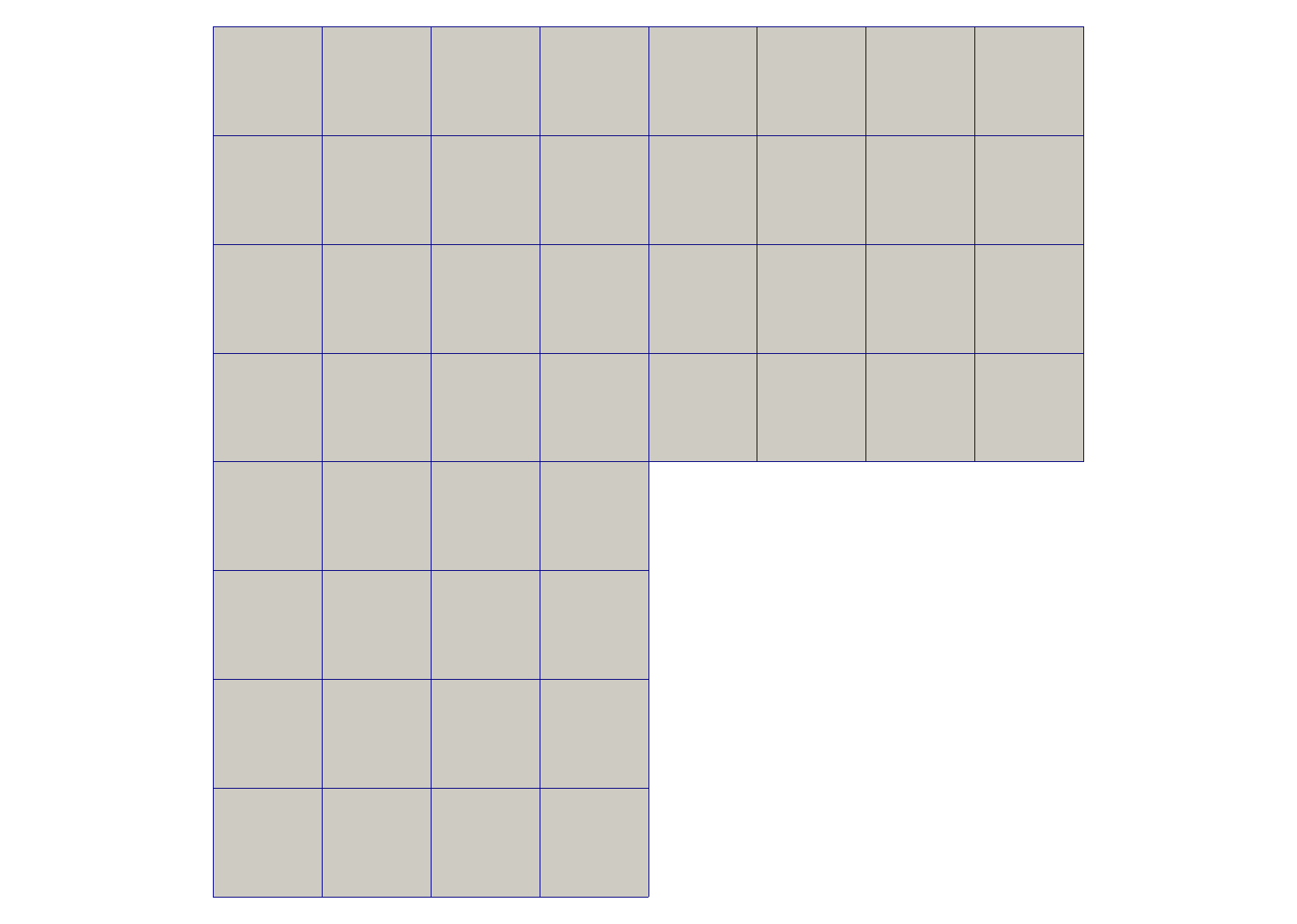
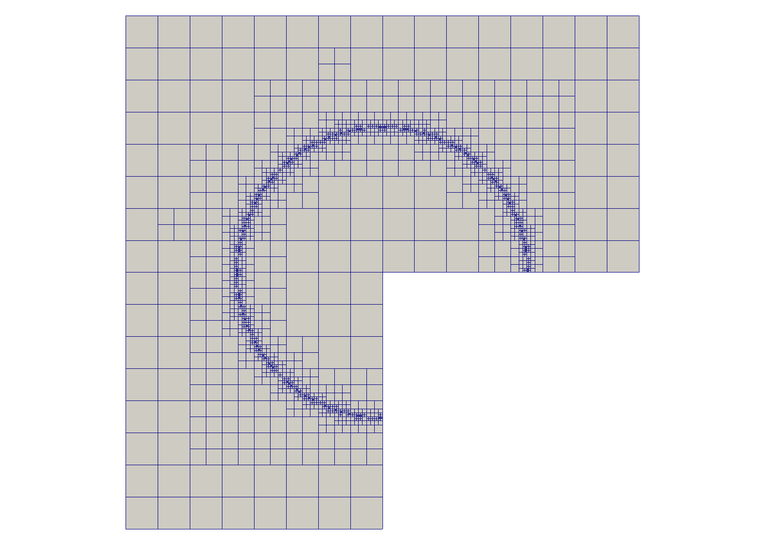
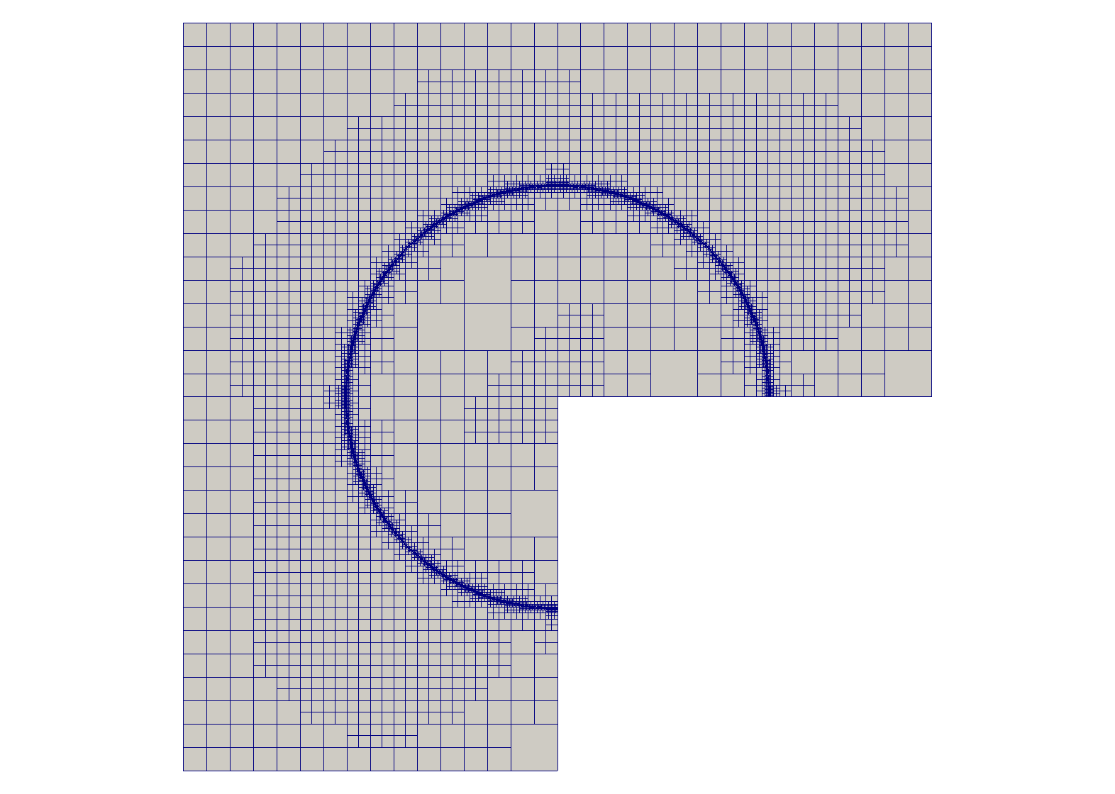
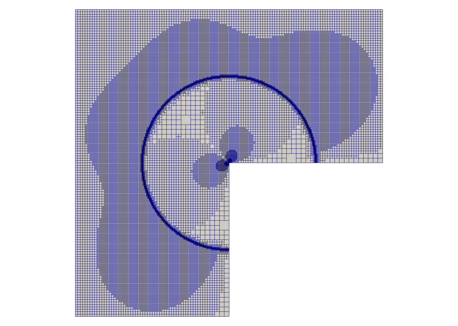
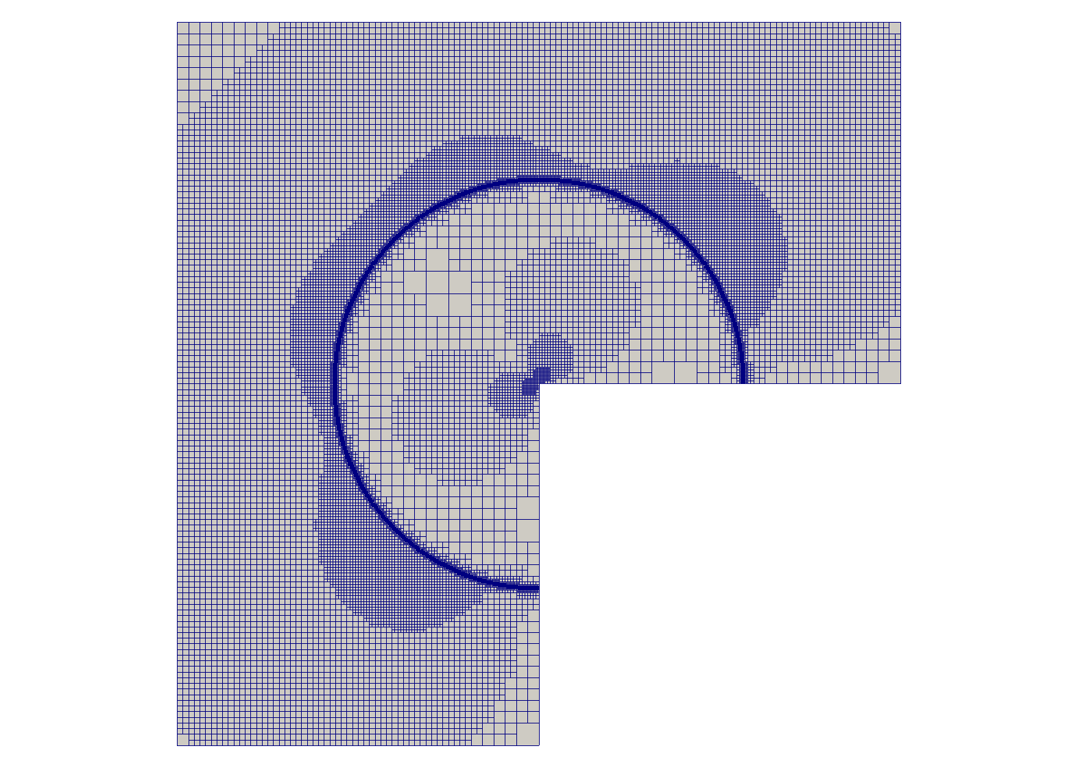
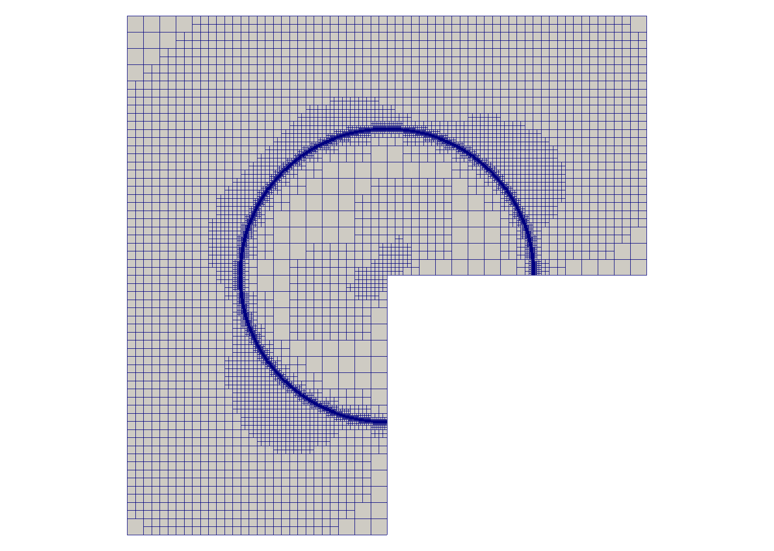
Fig. 6.1: Test 1 (L-shaped domain): Sequence of partitions (clockwise) generated by the algorithm DISC with integrability index $q=2$ for $A$, and parameters $\beta=0.7,\omega=0.8,\varepsilon_{0}=2$. The initial partition (top left) is made of uniform quadrilaterals without hanging nodes and all the subsequent partitions have at most one hanging node per side. The algorithm DISC refines at early stages only to capture the jump in the diffusion. The refinements caused by the singular behavior of the solution at the origin appear later in the adaptive process.

The parameters are chosen to be $\beta=0.7$, $\omega=0.8$ and $\varepsilon_{0}=2$. The standard AFEM loop in PDE is driven by error residual estimators together with a Dörfler marking strategy [14] with parameter $\theta=0.3$, which is rather conservative.

We now discuss the choice of $p$ for which Condition ${\bf p}$ is valid in view of Remark 1. Let $\Omega=\Omega_{1}\cup\Omega_{2}$ where $\Omega_{1}:=\{(\rho,\delta)\in\Omega:\rho\leq\rho_{0}/2\}$ and $\Omega_{2}:=\Omega\backslash\Omega_{1}$. The solution $u\in W^{1}(L_{p}(\Omega_{1}))$ for any $p<6$ in $\Omega_{1}$ and $u$ is Lipschitz in $\Omega_{2}$, whence Condition ${\bf p}$ is valid for $p<6$ in $\Omega_{1}$, i.e any $q=2p/(p-2)>3$, and $p=\infty$ in $\Omega_{2}$, i.e. any $q\geq 2$. Since the diffusion coefficient is constant on $\Omega_{1}$, it leads to zero approximation error of $A$ and we only have to handle the jump of $A$ across the circular line $\{\rho=\rho_{0}\}$ on $\Omega_{2}$.

Such a jump is never captured by the partitions, thereby making $A$ never piecewise smooth over partitions of ${\cal T}_{0}$ and preventing the use of a standard AFEM. It is easy to check that for any $1\leq q<\infty$, the matrix $A$ is in ${\cal M}^{1/q}(\mathcal{T}_{0},L_{q}(\Omega))$. Since the performance of DISC is reduced for larger $q$, according to (4.3), we should choose the smallest $q=2p/(p-1)$ compatible with $u\in W^{1}(L_{\infty}(\Omega_{2}))$, namely $q=2$ for $p=\infty$. The right hand side $f$ satisfies $f\in{\cal B}^{1/2}({\cal T}_{0},L_{2}(\Omega))\subset{\cal B}^{1/2}({\cal T}_{0},H^{-1}(\Omega))$, whereas the solution $u\in{\cal A}^{1/2}({\cal T}_{0},H^{1}_{0}(\Omega))$ because $u\in{\cal A}^{1/2}({\cal T}_{0},H^{1}(\Omega_{i}))$, $i=1,2$, and $\nabla u$ jumps over a Lipschitz curve [11, 12].

To test our theory, we take four different values of $p$ and thus the corresponding $q$ in our numerical experiments. For each of these different choices, Figure 6.2 (left) shows the decay of the energy error versus the number of degree of freedom in a $log-log$ scale. The experimental orders of convergence are

$$-0.19\quad\text{for}\quad q=6,\qquad-0.23\quad\text{for}\quad q=5,\qquad-0.35\quad\text{for}\quad q=3,\qquad-0.48\quad\text{for}\quad q=2,$$

in agreement with the approximability of $A$ stated above. These computational rates are close to the expected values $-1/q$, and reveal the importance of approximating and evaluating $A$ within subdomains with the smallest Lebesgue exponent $q$ possible. In this example $q=2$ yields an optimal rate of convergence for piecewise bilinear elements. Figure 6.2 (right) depicts the Galerkin solution after $6$ iterations of DISC for $q=2$. We finally point out that DISC with $q=\infty$, namely with $A$ being approximated in $L_{\infty}(\Omega)$, cannot reduce the pointwise error in $A$ beyond $3.96$ computationally which is consistent with the jump of $A$. As a consequence, any call of COEFF with any smaller target tolerance and $q=\infty$ does not converge.

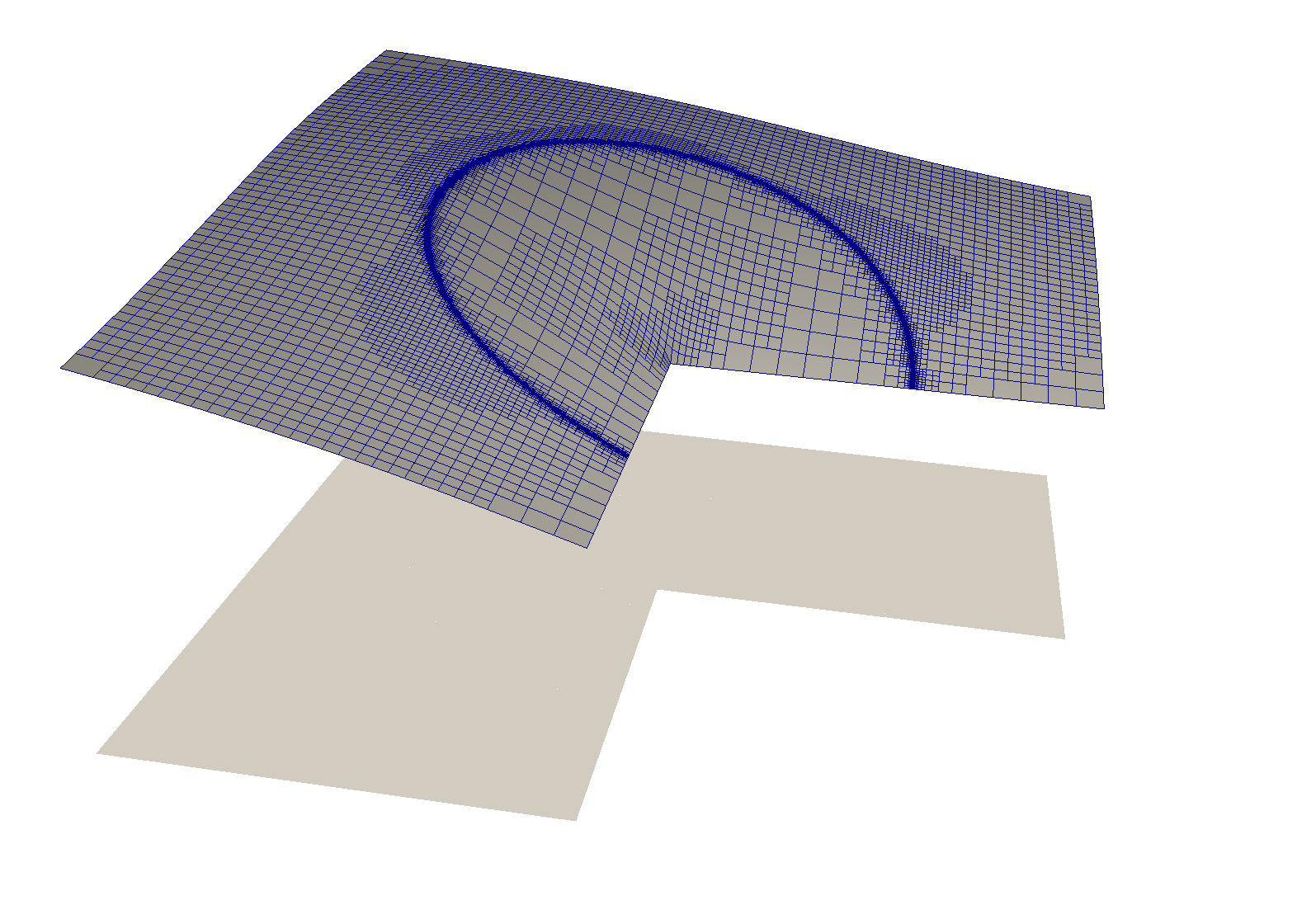
Fig. 6.2: Test 1 (L-shaped domain): (Left) Energy error versus number of degrees of freedom for values of $q=2,3,5,6$. The optimal rate of convergence is recovered for $q=2$. (Right) The Galerkin solution together with the underlying partition after $6$ iterations of the algorithm DISC with $q=2$. The discontinuity of $A$ is never captured by the partitions and the singularities of both $A$ and $\nabla u$ drive the refinements.

6.2 Test 2: Checkerboard

We now examine DISC with an example which does not allow for $q=2$. In this explicit example, originally suggested by Kellogg [16], the line discontinuity of the diffusion matrix $A$ meets the singularity of the solution $u$. Let $\Omega=(-1,1)^{2}$, $A=aI$, where $I$ is the $2\times 2$ identity matrices and

$$a(x,y)=\left\{\begin{array}[]{ll}b&\qquad\mathrm{when}\quad(x-\frac{\sqrt{2}}{10})(y-\frac{\sqrt{2}}{10})\geq 0\\ 1&\qquad\mathrm{otherwise,}\end{array}\right.$$

with $b>0$ given. The forcing is chosen to be $f\equiv 0$ so that with appropriate boundary conditions, the solution $u$ in polar coordinates $(\rho,\delta)$ centered at the point $(\frac{\sqrt{2}}{10},\frac{\sqrt{2}}{10})$ reads

$$u(\rho,\delta)=\rho^{\alpha}\mu(\delta).$$

where $0<\alpha<2$ and

$$\mu(\delta):=\left\{\begin{array}[]{ll}\cos((\frac{\pi}{2}-\sigma)\alpha)\cos((\delta-\frac{\pi}{4})\alpha)&\qquad\mathrm{when}\quad 0\leq\delta<\frac{\pi}{2},\\ \cos(\frac{\pi}{4}\alpha)\cos((\delta-\pi+\sigma)\alpha)&\qquad\mathrm{when}\quad\frac{\pi}{2}\leq\delta<\pi,\\ \cos(\alpha\sigma)\cos((\delta-\frac{5\pi}{4})\alpha)&\qquad\mathrm{when}\quad\pi\leq\delta<\frac{3\pi}{2},\\ \cos(\frac{\pi}{4}\alpha)\cos((\delta-\frac{3\pi}{2}-\sigma)\alpha)&\qquad\mathrm{when}\quad\frac{3\pi}{2}\leq\delta<2\pi.\end{array}\right.$$

The parameters $b$, $\alpha$ and $\sigma$ satisfy the non linear relations

$$b=-\tan((\frac{\pi}{2}-\sigma)\alpha)\cot(\frac{\pi}{4}\alpha),\quad\frac{1}{b}=-\tan(\frac{\pi}{4}\alpha)\cot(\sigma\alpha),\quad b=-\tan(\alpha\sigma)\cot(\frac{\pi}{4}\alpha)$$

together with the constraints

$$\max(0,\pi(\alpha-1))<\frac{\pi}{2}\alpha<\min(\pi\alpha,\pi),\qquad\max(0,\pi(1-\alpha))<-2\alpha\sigma<\min(\pi,\pi(2-\alpha)).$$

We stress that the singular solution $u\in H^{1+s}(\Omega)$, $s<\alpha$, yet $u\in\mathcal{A}^{1/2}(H^{1}_{0}(\Omega))$ [20]. However, the discontinuity of $A$ meets the singularity of $u$ and Remark 1 does no longer apply. In this case we have $p<2/(1-\alpha)$ and $s_{A}=1/q=(p-2)/2p<\alpha/2$.

We challenge the algorithm DISC with the approximate parameters

$$\alpha=0.25,\quad b\approx 25.27414236908818,\quad\sigma\approx-5.49778714378214,$$ (6.2)

which correspond to $p<8/3$ and $s_{A}<1/8$. We exploit (6.1) and choose $\bar{A}$ to be the meanvalue of $A$ element-by-element. We report the experimental order of convergence (EOC) of the energy error against the number of degrees of freedom in Fig. 6.3 together with the solution at the final stage. The asymptotic EOC (averaging the last 6 points) is $-0.47$, which is about optimal and much better than the expected value $s_{A}\approx-0.125$. On the other hand, the preasymptotic EOC (without the last 6 points) is about $-0.2$. We will give a heuristic explanation of this superconvergence rate in the following subsection. We now conclude with Fig. 6.4 which depicts quadrilateral partitions at stages $k=0,7,22$.

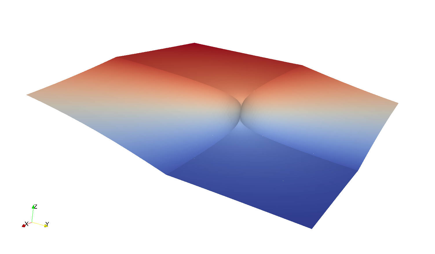
Fig. 6.3: Test 2 (Checkerboard): The parameters are chosen so that the solution $u\in H^{1+s}(\Omega)$, $s<0.25$. (Left) Energy error versus number of degrees of freedom. The optimal rate of convergence $\approx-0.5$ is recovered. (Right) The Galerkin solution together with the underlying partition after $6$ iterations of the algorithm DISC. The discontinuity of $A$ is never captured by the partitions and the singularities of both $A$ and $\nabla u$ drive the refinements.

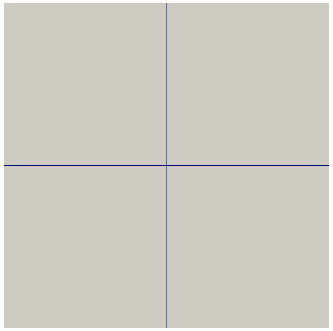
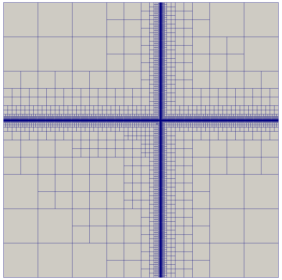
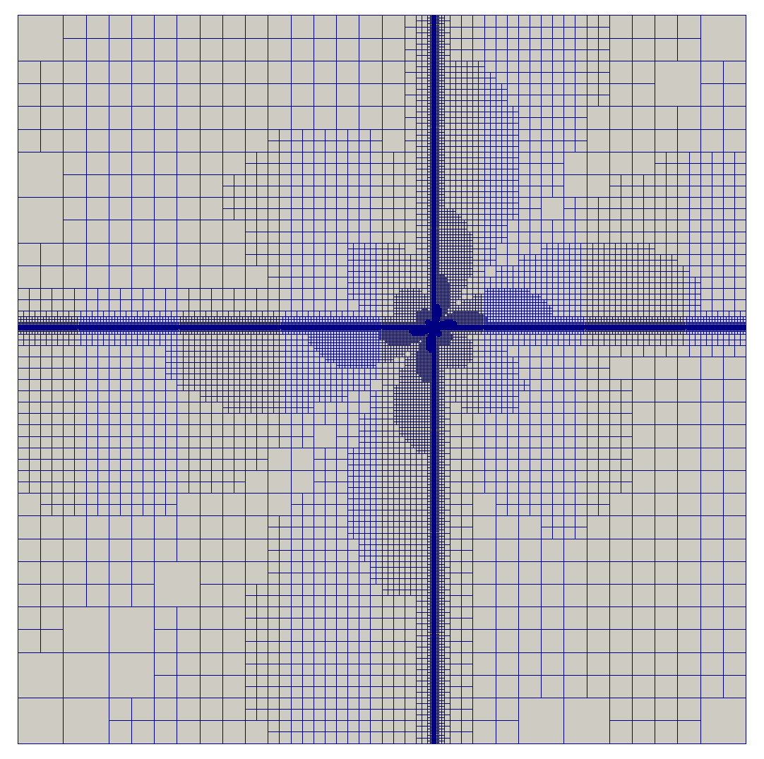
Fig. 6.4: Test 2 (Checkerboard): Sequence of partitions (from left to right) generated by DISC with $\omega=0.8$. The initial partition (first) is made of four quadrilaterals, The algorithm refines at early stages only to capture the discontinuity in the diffusion coefficient (second). Later the singularity of $u$ comes into play and, together with that of $A$, drives the refinement (third). The corresponding subdivision consists of $5$ million degrees of freedom. The smallest cell has a diameter of $2^{-8}$ which illustrates the strongly graded mesh constructed by DISC.

6.3 Performance of DISC with Interacting Jump and Corner Singularities

We finally give a heuristic explanation to the surprising superconvergence behavior of DISC in Test 2. Let $u\approx\rho^{\alpha}$, with $0<\alpha<1$, be the prototype solution such as that of Section 6.2. Let $A$ be a discontinuous diffusion matrix with discontinuity across a Lipschitz curve $\Gamma$ emanating from the origin, and let $\bar{A}$ be its local meanvalue.

Let $\omega_{j}$ be the annulus $\{x\in\Omega:2^{-(j+1)}<\rho=|x|<2^{-j}\}$ for $0\leq j\leq J$ and set $\omega_{J+1}:=\{x\in\Omega:|x|<2^{-(J+1)}\}$. We assume that $c^{-1}h_{j}^{2}\leq|T|\leq ch_{j}^{2}$ for each element $T$ within $\omega_{j}$ touching $\Gamma$, where $c$ is a constant independent of $j$ and the total number of cells $N$. Revisiting the proof of the perturbation theorem (Theorem 1), we realize that the error $E_{A}$ due to the approximation of $A$ can be decomposed as follows:

$$E_{A}^{2}:=\|(A-\bar{A})\nabla u\|_{L_{2}(\Omega)}^{2}{\color[rgb]{0,0,0}{\approx}}\sum_{j=0}^{J+1}\|(A-\bar{A})\nabla u\|_{L_{2}(\omega_{j})}^{2}=\sum_{j=0}^{J+1}\delta_{j}^{2},\qquad\delta_{j}:=\|(A-\bar{A})\nabla u\|_{L_{2}(\omega_{j})}.$$

We choose $q=2$ and $p=\infty$ away from the origin which implies that the contribution $\delta_{j}$ within $\omega_{j}$ is estimated by

$$\delta_{j}\leq\|A-\bar{A}\|_{L_{2}(\omega_{j})}\|\nabla u\|_{L_{\infty}(\omega_{j})},\quad 0\leq j\leq J.$$

The first term is simply the square root of the area around the interface and within $\omega_{j}$, which amounts to $\|A-\bar{A}\|_{L_{2}(\omega_{j})}\approx\big{(}h_{j}2^{-j}\big{)}^{1/2}\approx\big{(}N_{j}^{-1}2^{-2j}\big{)}^{1/2},$ with $N_{j}\approx h_{j}^{-1}2^{-j}$ being the number of elements touching $\Gamma$ within $\omega_{j}$. The second term reduces to $\|\nabla u\|_{L^{\infty}(\omega_{j})}\approx 2^{-j(\alpha-1)},$ whence

$$\delta_{j}\approx N_{j}^{-1/2}2^{-j\alpha}.$$

We further assume error equidistribution, which entails $\delta_{j}^{2}\approx\Lambda$ constant independent of $j$. This implies

$$N_{j}\approx\Lambda^{-1}2^{-2j\alpha}\qquad\Rightarrow\qquad N\approx\sum_{j=0}^{J}N_{j}\approx\Lambda^{-1}\sum_{j=0}^{J}2^{-2j\alpha}\approx\Lambda^{-1}$$

because $\alpha>0$. It remains to determine the value of $J$. On $\omega_{J+1}$ we have $\nabla u\in L_{p}$, $p<\frac{2}{1-\alpha}$, so that with $q=\frac{2p}{p-2}$, the contribution from $\omega_{J+1}$ is estimated by

$$\delta_{J+1}^{2}\leq\|A-\bar{A}\|^{2}_{L_{q}(\omega_{J+1})}\|\nabla u\|^{2}_{L_{p}(\omega_{J+1})}\preceq|\omega_{J+1}|^{2/q}\preceq 2^{-\frac{4J}{q}}$$

with a hidden constant that blows up as $q$ approaches the limiting value $2/\alpha$. Matching the error $\delta_{J+1}^{2}$ with $\Lambda$ gives rise to the relation

$$N\approx 2^{4J/q}\qquad\Rightarrow\qquad J\approx\log N.$$

We thus conclude that

$$E_{A}\approx\big{(}J/N\big{)}^{1/2}\approx N^{-1/2}|\log N|^{1/2}.$$

The ensuing mesh has a graded meshsize $h_{j}\approx N^{-1}2^{-j(1-2\alpha)}$ towards the origin provided $\alpha<1/2$; if $\alpha\geq 1/2$ then uniform refinement suffices. Such a graded mesh cannot result from the application of COEFF because it only measures the jump discontinuity of $A$ which is independent of the distance to the origin.

However, the refinement due to PDE could be much more severe because the best bilinear approximation $\hat{U}$ of $u$ on $T\subset\omega_{j}$ reads

$$E_{u}(T)^{2}:=\|u-\hat{U}\|_{H^{1}(T)}^{2}\approx h_{j}^{2}2^{2j(2-\alpha)}$$

and equidistribution $E_{u}(T)\approx\lambda$ (constant) yields a graded meshsize $h_{j}\approx\lambda 2^{-j(2-\alpha)}$. This grading is stronger than that due to $A$ and asymptotically dominates. This in turn explains the preasymptotic EOC of Fig. 6.3 and the quasi-optimal asymptotic EOC also of Fig. 6.3.

References

- [1] W. Bangerth, R. Hartmann, and G. Kanschat. deal.II—a general-purpose object-oriented finite element library. ACM Trans. Math. Software, 33(4):Art. 24, 27, 2007.
- [2] P. Binev, W. Dahmen, and R. DeVore. Adaptive finite element methods with convergence rates. Numer. Math., 97(2):219–268, 2004.
- [3] P. Binev, W. Dahmen, R. DeVore, and P. Petrushev. Approximation classes for adaptive methods. Serdica Math. J., 28(4):391–416, 2002. Dedicated to the memory of Vassil Popov on the occasion of his 60th birthday.
- [4] P. Binev and R. DeVore. Fast computation in adaptive tree approximation. Numer. Math., 97(2):193–217, 2004.
- [5] M. Sh. Birman and M.Z. Solomyak. Piecewise-polynomial approximations of functions of the classes . Mat. Sb. (N.S.), 73(115)(3):331–355, 1967.
- [6] A. Bonito, J.M. Cascón, P. Morin, and R.H. Nochetto. Afem for geometric pde: The laplace-beltrami operator. In Franco Brezzi, Piero Colli Franzone, Ugo Gianazza, and Gianni Gilardi, editors, Analysis and Numerics of Partial Differential Equations, volume 4 of Springer INdAM Series, pages 257–306. Springer Milan, 2013.
- [7] A. Bonito and R.H. Nochetto. Quasi-optimal convergence rate of an adaptive discontinuous Galerkin method. SIAM J. Numer. Anal., 48(2):734–771, 2010.
- [8] S.C. Brenner and L. R. Scott. The Mathematical Theory of Finite Element Methods, volume 15 of Texts in Applied Mathematics. Springer, New York, third edition, 2008.
- [9] J. M. Cascón, Ch. Kreuzer, R. H. Nochetto, and K. G. Siebert. Quasi-optimal convergence rate for an adaptive finite element method. SIAM J. Numer. Anal., 46(5):2524–2550, 2008.
- [10] A. Cohen, W. Dahmen, I. Daubechies, and R. DeVore. Tree approximation and optimal encoding. Appl. Comput. Harmon. Anal., 11(2):192–226, 2001.
- [11] A. Cohen, R. DeVore, and R. H. Nochetto. Convergence Rates of AFEM with Data. Found. Comput. Math., 12(5):671–718, 2012.
- [12] S. Dahlke and R.A. DeVore. Besov regularity for elliptic boundary value problems. Comm. Partial Differential Equations, 22(1-2):1–16, 1997.
- [13] M. C. Delfour and J.-P. Zolésio. Shapes and geometries, volume 22 of Advances in Design and Control. Society for Industrial and Applied Mathematics (SIAM), Philadelphia, PA, second edition, 2011. Metrics, analysis, differential calculus, and optimization.
- [14] W. Dörfler. A convergent adaptive algorithm for Poisson’s equation. SIAM J. Numer. Anal., 33(3):1106–1124, 1996.
- [15] D. Jerison and C.E. Kenig. The inhomogeneous Dirichlet problem in Lipschitz domains. J. Funct. Anal., 130(1):161–219, 1995.
- [16] R. B. Kellogg. On the Poisson equation with intersecting interfaces. Applicable Anal., 4:101–129, 1974/75. Collection of articles dedicated to Nikolai Ivanovich Muskhelishvili.
- [17] S. Larsson and V. Thomée. Partial differential equations with numerical methods, volume 45 of Texts in Applied Mathematics. Springer-Verlag, Berlin, 2009.
- [18] N.G. Meyers. An -estimate for the gradient of solutions of second order elliptic divergence equations. Ann. Scuola Norm. Sup. Pisa (3), 17:189–206, 1963.
- [19] P. Morin, R.H. Nochetto, and K.G. Siebert. Convergence of adaptive finite element methods. SIAM Rev., 44(4):631–658 (electronic) (2003), 2002. Revised reprint of “Data oscillation and convergence of adaptive FEM” [SIAM J. Numer. Anal. 38 (2000), no. 2, 466–488 (electronic); MR1770058 (2001g:65157)].
- [20] R.H. Nochetto, K.G. Siebert, and A. Veeser. Theory of adaptive finite element methods: an introduction. In Multiscale, nonlinear and adaptive approximation, pages 409–542. Springer, Berlin, 2009.
- [21] R. Stevenson. Optimality of a standard adaptive finite element method. Found. Comput. Math., 7(2):245–269, 2007.
- [22] R. Stevenson. The completion of locally refined simplicial partitions created by bisection. Math. Comp., 77(261):227–241 (electronic), 2008.