Perspectives on Intracluster Enrichment and the Stellar Initial Mass Function in Elliptical Galaxies

Abstract

Stars formed in galaxy cluster potential wells must be responsible for the high level of enrichment measured in the intracluster medium (ICM); however, there is increasing tension between this truism and the parsimonious assumption that the stars in the generally old population studied optically in cluster galaxies emerged from the same formation sites at the same epochs. We construct a phenomenological cluster enrichment model to demonstrate that ICM elemental abundances are underestimated by a factor $>2$ for standard assumptions about the stellar population – a discrepancy we term the “cluster elemental abundance paradox”. Recent evidence of an elliptical galaxy IMF skewed to low masses deepens the paradox. We quantify the adjustments to the star formation efficiency and initial mass function (IMF), and SNIa production efficiency, required to resolve this while being consistent with the observed ICM abundance pattern. The necessary enhancement in metal enrichment may, in principle, originate in the observed stellar population if a larger fraction of stars in the supernova-progenitor mass range form from an initial mass function (IMF) that is either bottom-light or top-heavy, with the latter in some conflict with observed ICM abundance ratios. Other alternatives that imply more modest revisions to the IMF, mass return and remnant fractions, and primordial fraction, posit an increase in the fraction of $3-8~{}{\mathrm{M}}_{\sun}$ stars that explode as SNIa or assume that there are more stars than conventionally thought – although the latter implies a high star formation efficiency. We discuss the feasibility of these various solutions and the implications for the diversity of star formation in the universe, the process of elliptical galaxy formation, and the origin of this “hidden” source of ICM metal enrichment.

1. Context

The hot plasma that pervades the volume of the most massive galaxy clusters – the intracluster medium (ICM) – provides a wealth of diagnostic data on the process of galaxy formation in structures formed from the largest primordial density fluctuations to have entered the nonlinear regime and undergone gravitational collapse. The history and efficiency of star formation, and the effects of interactions among galaxies and between galaxies and the environment in the form of infall, outflow, and dynamical stripping, are reflected in the thermal and chemical properties of the ICM – both in individual systems and in the evolving population of clusters.

In massive ($>10^{14}~{}{\mathrm{M}}_{\sun}$) clusters, the ICM dominates the baryon inventory and accounts for $>10$% of the total matter content (e.g., Laganá et al. 2011). The discovery that cluster gas fractions expected to be representative of the universe as a whole exceed $\Omega_{baryon}$ precipitated a crisis referred to as the “baryon catastrophe” when combined with the assumption of a matter-dominated universe and evidence for, and the inflationary prediction of, a flat universe – i.e. $\Omega_{matter}=1$ (Fabian, 1991; White et al., 1993). Of course this paradox was resolved by the discovery of dark energy and the concordance cosmology which reconciles a flat universe with a reduced $\Omega_{matter}$. The cosmic baryon matter fraction is now accurately determined, $\Omega_{baryon}/\Omega_{matter}=0.17$ (Jarosik et al., 2011), with a relatively modest percentage of the baryons collapsed into stars, $\Omega_{stars}/\Omega_{matter}\approx 0.0074-0.011$ (Gallazzi et al., 2008).

However a related paradox persists to this day. While a solar nucleosynthetic yield (i.e., star formation ultimately producing the amount of metals necessary to enrich one solar mass to solar abundances) is sufficient only to enrich baryons to average abundance of $<0.1$ on a universal scale, cluster baryons are enriched in Fe (and other elements) to $\sim$half-solar (Tamura et al., 2004; de Plaa et al., 2007; Leccardi & Molendi, 2008; Bregman et al., 2010; Matsushita, 2011; Baldi et al., 2012; Andreon, 2012). Star formation in cluster galaxies is evidently more efficient than in the field; however, a discrepancy between cluster metals and the number of stars evidently available to produce these metals was noted following the very first detection of intraclcuster Fe by Mitchell et al. (1976) and Serlemitsos et al. (1977) (Vigroux, 1977; Rothenflug et al., 1984; Rothenflug & Arnaud, 1985; Arnaud et al., 1992). This discordance was confirmed and quantified in detail following the groundbreaking accuracy and range of abundance measurements made with the ASCA X-ray Observatory (Loewenstein & Mushotzky, 1996; Mushotzky & Loewenstein, 1997; Pagel, 1999, 2002; Lin et al., 2003; Finoguenov et al., 2003; Portinari et al., 2004; Lin & Mohr, 2004; De Lucia et al., 2004; Loewenstein, 2006; Maoz et al., 2010; Bregman et al., 2010). This may be framed in terms of the Fe-mass-to-light ratio (Arnaud et al., 1992; Renzini et al., 1993): for $M_{*}/L_{B}=5$ a solar yield corresponds to $M_{Fe}/L_{B}\sim 0.0065$ – falling short by a factor of 5 or more compared to what is measured (Sakuma et al., 2011; Sato et al., 2012).

To resolve this “cluster elemental abundance paradox” one generally must conclude that there was more star formation in clusters than conventionally estimated, and/or that star formation in galaxy clusters has an enhanced efficiency of producing supernova progenitors and synthesizing metals. “Missing” stars may take the form of low surface brightness intracluster light (ICL), inferred both from observations (Zaritsky et al., 2004; Lin & Mohr, 2004; Gonzalez et al., 2007; Krick & Bernstein, 2007) and simulations (Puchweine al., 2010; Rudick et al., 2011). Recent literature includes a large range in calculated star-to-ICM ratios primarily due to divergent ICL estimates, but also to different assumed stellar mass-to-light ratios. A stellar initial mass function (IMF) that is relatively top heavy increases both the ratio of stars formed, and of metals created, to present-day light. Such an IMF may be bimodal in nature (Elbaz et al., 1995; Larson, 1998; Moretti et al., 2003), the second mode perhaps associated with a distinct pre-enrichment population (Bregman et al., 2010) where Population III hypernovae (Loewenstein, 2001) may play a role. Given the conventional wisdom that most ICM metals originate in elliptical galaxies (Arnaud et al., 1992), this problem clearly connects to the fundamental galaxy formation questions of the IMF in ellipticals and the transport of material from these galaxies into intergalactic space.

In this paper we undertake a fresh and comprehensive, though generic, examination of the metal inventory in the ICM of rich galaxy clusters. We focus on addressing a single well-defined, though multifaceted, question: what characteristics of the stellar population are necessary to produce the observed level of ICM enrichment? In doing so we address issues related to the IMF, star and galaxy formation efficiency, galactic winds, the astrophysics of supernova progenitors and explosions, and the apportionment of products of different supernova types into stars and ICM. Section 2 quantitatively summarizes the cluster elemental abundance paradox.

In Section 3, where a standard IMF is assumed, the level of enrichment and abundance pattern are related to phenomenological parameters that encapsulate the star formation efficiency, and the demographics of supernovae and the success of stars in locking up the products of their explosion. Substantial departures from standard values are required to match observations. In Section 4, we cast a wider net by considering the effects on ICM enrichment of a wide range of IMFs in the context of a self-consistent galaxy chemical evolution treatment that accounts for the relevant astrophysical quantities. When juxtaposed with recent evidence for an IMF in elliptical galaxies that produces fewer metals than a local IMF, this analysis reinforces and clarifies the conflict between the ICM metallicity and the characteristics of the stellar population generally assumed responsible for ICM enrichment. Results and their implications are discussed, and conclusions summarized, in Section 5.

2. The Cluster Elemental Abundance Paradox Quantified

2.1. Basics

Consider the total baryon mass in a cluster of galaxies within some sufficiently large radius that it may be considered a closed box in the chemical evolution sense – that is, all products resulting from the transformation of some of this gas into stars (including the stars themselves) are contained within this radius. There is direct evidence that this is a good approximation for sufficiently massive clusters if invoked at radii that are a significant fraction of the virial radius, based on the consistency between the total cluster baryon fraction and the universal value mentioned above (Landry et al., 2012), perhaps with a $\sim 10$% “depletion” correction at $r_{500}$ (the radius within which the average mass density is 500 times the critical density); see Gonzalez et al. (2007); Pratt et al. (2009); Giodini et al. (2009); Ade et al. (2013); Planelles et al. (2013); Eckert et al. (2013). Presumably this is a result of the extreme depth of their gravitational potential wells. However it is possible that this also applies to galaxy groups, and perhaps even giant elliptical galaxies if one could inventory the gas all the way out to the virial radius (and perhaps beyond, if entropy injection has dispersed the gas distribution).

We define the overall efficiency of converting gas into stars, $\varepsilon_{sf}$, such that the total mass in stars formed (regardless of where) is

$$M_{*,form}=\varepsilon_{sf}\,M_{baryon},$$ (1)

where $M_{baryon}$ is the total baryon mass being considered. At the present time the total mass in stars, whether contained in individual cluster galaxies (including the brightest cluster galaxy – BCG) or associated with intracluster light (ICL), is

$$M_{*}=M_{baryon}\,\varepsilon_{sf}\,(1-r_{*}),$$ (2)

and the mass in gas is

$$M_{gas} =M_{baryon}-M_{*}$$ (3)

$$=M_{baryon}\left[1-\varepsilon_{sf}(1-r_{*})\right],$$ (4)

where $r_{*}$ is the stellar “mass return fraction” – the fraction of the mass previously formed into stars recycled back into gas. For massive clusters one may neglect the distinction between the total mass in gas and the mass in the ICM, and henceforth we equate $M_{gas}$ with $M_{ICM}$. The star formation efficiency, in terms of the observable $M_{ICM}/M_{*}$ is

$$\varepsilon_{sf}=(1-r_{*})^{-1}\left(1+\frac{M_{ICM}}{M_{*}}\right)^{-1}.$$ (5)

We consider the enrichment of cluster baryons in chemical elements released in supernova explosions, i.e. those of atomic number $A\geq 8$. It is straightforward to extend the analysis to elements statically synthesized in intermediate mass stars; however, the elements (C, N) to which this applies are not well-constrained by current X-ray observations.

Both the overall level of baryon enrichment (that is, the metallicity) and the abundance pattern are determined by the total number of supernovae and their nucleosynthetic yields. We separate the enrichment contributions of the two main classes of supernovae – Type Ia supernovae (SNIa) that result from the explosion of a white dwarf, and core collapse supernovae (SNcc). Their total numbers may be expressed as

$$N^{cc}=\eta^{cc}\,M_{*,form}$$ (6)

and

$$N^{Ia}=\eta^{Ia}M_{*,form};$$ (7)

where $\eta^{cc}$ and $\eta^{Ia}$ are, respectively, the specific numbers of SNcc and SNIa explosions per star formed. It is useful to define the total supernova number, supernova ratio, and SNIa fraction as follows:

$$N^{SN} =N^{cc}+N^{Ia}$$ (8)

$$=\eta^{SN}~{}(1-r_{*})^{-1}M_{*},$$ (9)

where

$$\eta^{SN}=\eta^{cc}+\eta^{Ia};$$ (10)

$$R^{SN}\equiv\frac{\eta^{Ia}}{\eta^{cc}};$$ (11)

and

$$f^{Ia}\equiv\frac{\eta^{Ia}}{\eta^{SN}}=\frac{R^{SN}}{1+R^{SN}}.$$ (12)

Note that the number of SN per unit mass in the ICM is

$$\frac{N^{SN}}{M_{ICM}}=\eta^{SN}~{}(1-r_{*})^{-1}\frac{f_{*}}{f_{ICM}},$$ (13)

where $f_{*}$ and $f_{ICM}$ are the present-day mass fractions of stars and gas: $f_{*}/f_{ICM}=M_{*}/M_{ICM}$.

2.2. Stars and Supernovae

A combination of theoretical and empirical considerations enter into determination of the stellar and supernovae parameters. Star formation is not sufficiently well-understood to allow an a priori estimate of $\varepsilon_{sf}$, and $M_{*}$ is estimated from observations of cluster starlight in galaxies and intracluster space. To convert to mass, stellar population synthesis can be employed, involving assumptions about the IMF – among many other factors. The mass-to-light ratio in individual galaxies can also be inferred from dynamical modeling of stellar velocity dispersion distributions. The mass return fraction, $r_{*}$, may be calculated from the IMF, star formation history (SFH), and relation of stellar remnant mass to progenitor mass for individual stars estimated from stellar evolution theory and observations in the Galaxy. The SNcc efficiency, ${\eta^{cc}}$, depends on the IMF and range of masses that result in core collapse explosions. Although one may model the time-dependence of the SNIa rate from assumptions about the binary star progenitor configuration and the distributions of binary mass ratios and separations, the normalization is difficult to estimate a priori. Empirical estimates of ${\eta^{Ia}}$ (and ${\eta^{cc}}$) are emerging from supernova surveys that also constrain the distribution of delay times from the observed evolution of the SNIa rate (Maoz & Mannucci, 2012; Sand et al., 2012). Estimation of these fundamental quantities – $M_{*}$, $r_{*}$, ${\eta^{Ia}}$, ${\eta^{cc}}$ – in principle requires a convolution and a time-integration over an evolving galaxy population with disparate SFHs and, conceivably, IMFs. A first order approximation treats the ensemble stellar population as a single simple population of stars formed at some (high) redshift with a common IMF – an approximation most suitable for rich clusters where the total galaxy mass is most dominated by elliptical galaxies.

We can insert some reasonable values to get a sense for the expected level of supernova enrichment and relative contribution from the two classes of supernovae. For a “diet Salpeter” IMF that represents a simple alteration – proposed as a means of reconciliation with the observed relative frequency of $\sim$subsolar mass stars (Bell & de Jong, 2001) – of the classic single-slope Salpeter function (Salpeter, 1955), $\eta^{Ia}\sim 0.002$ (Maoz & Mannucci, 2012), $r_{*}\sim 0.35$ for an old stellar population (Fardal et al., 2007; O’Rourke et al., 2011), and $\eta^{cc}\sim 0.008$ (Maoz & Mannucci, 2012; Botticella et al., 2012; Dahlen et al., 2012).

One then predicts $R^{SN}\sim 0.25$ ($f^{Ia}\sim 0.2$) and $\eta^{SN}\sim 0.01$. For massive clusters (i.e., $M_{500}\equiv M(r_{500})>10^{14}~{}{\mathrm{M}}_{\sun}$), recent studies report a range in stellar mass fraction evaluated at $r_{500}$, reflecting different treatments of ICL and in conversion from light to mass (Zhang et al., 2011), with $f_{*}/f_{ICM}$ typically $\sim 0.1$ (Lin et al., 2003; Gonzalez et al., 2007; Giodini et al., 2009; Ettori et al., 2009; Dai et al., 2010; Andreon, 2010; Bregman et al., 2010; Laganá et al., 2011; Balogh et al., 2011; Zhang et al., 2011; Lin et al., 2012) (though with substantial systematic uncertainty and study-to-study variation; see Leauthaud et al. (2012)), and evidence of an increase in magnitude and scatter with decreasing cluster mass. The resulting total number of supernova explosions per solar mass of ICM is $\sim 1.5\times 10^{-3}(10f_{*}/f_{ICM})~{}{\mathrm{M}}_{\sun}^{-1}$.

2.3. Application to the ICM

The equation for the mass of the $ith$ element in the ICM, $M_{i}$, in terms of the number of SNIa and SNcc that enrich the ICM, $N^{Ia}$ and $N^{cc}$, and the yields per SNIa and SNcc, $y_{i}^{Ia}$ and $\langle y_{i}^{cc}\rangle$, is

$$M_{i}=N^{cc}\langle y_{i}^{cc}\rangle+N^{Ia}y_{i}^{Ia}=N^{SN}(1+R^{SN})^{-1}(\langle y_{i}^{cc}\rangle+R^{SN}y_{i}^{Ia}),$$ (14)

where, as defined above, $R^{SN}\equiv N^{Ia}/N^{cc}$ and $N^{SN}\equiv N^{Ia}+N^{cc}$. The IMF($\phi$)-averaged SNcc yield is

$$\langle y_{i}^{cc}\rangle=\frac{\int^{m_{up}}_{m_{cc}}dm\phi(m)y_{i}^{cc}(m)}{\int^{m_{up}}_{m_{cc}}dm\phi(m)},$$ (15)

where $m_{cc}$ and $m_{up}$ are the lower and upper limits for the masses of SNcc progenitors, and a single universal set of SNIa yields is assumed. Despite a plethora of IMF parameterizations (Kroupa et al., 2012), there is general consensus that a Salpeter slope (Salpeter, 1955), $\phi\sim m^{-2.35}$ applies at the high mass end relevant for SNcc – at least for star formation under “normal” conditions.

The resulting mass fraction in the ICM (mass $M_{ICM}$) of the $ith$ element, $f_{i}$, is

$$f_{i}\equiv\frac{M_{i}}{M_{ICM}}=\frac{N^{SN}}{M_{ICM}}(1+R^{SN})^{-1}(\langle y_{i}^{cc}\rangle+R^{SN}y_{i}^{Ia}),$$ (16)

and the mass fraction relative to the solar mass fraction,

$$\frac{f_{i}}{f_{i\sun}}=\frac{N^{SN}}{M_{ICM}}(1+R^{SN})^{-1}\left(\frac{\langle y_{i}^{cc}\rangle}{f_{i\sun}}+R^{SN}\frac{y_{i}^{Ia}}{f_{i\sun}}\right).$$ (17)

The relationship between mass fraction, $f_{i}$, and abundance, $z_{i}$, of the $ith$ element (the number of atoms of element $i$ relative to that of H, i.e. the entries in standard abundance tables) is $z_{i}=(f_{i}/X)(A_{i}/A_{H})^{-1}$, where $X$ and $A_{H}$ are the hydrogen mass fraction and atomic weight ($A_{H}=1.008$ AMU) and $A_{i}$ the atomic weight of the $ith$ element. Relative to solar, the abundance is

$$\frac{z_{i}}{z_{i\sun}}=\frac{X_{\sun}}{X}\frac{f_{i}}{f_{i\sun}}\approx\frac{f_{i}}{f_{i\sun}},$$ (18)

where $f_{i\sun}=z_{i\sun}X_{\sun}(A_{i}/A_{H})$, and the approximation $X=X_{\sun}$ is invoked – an approximation that is valid as long as the total mass fraction of metals ($<2$% for solar abundances) is small and the He abundance is fixed. $X$ for various solar standard abundance sets is given in Table 4 of Asplund et al. (2009).

Finally, the abundance relative to solar is expressed as

$$Z_{i}\equiv\frac{z_{i}}{z_{i\sun}}=\frac{N^{SN}}{M_{ICM}}(1+R^{SN})^{-1}(\langle y_{i}^{cc^{\prime}}\rangle+R^{SN}y_{i}^{Ia^{\prime}})$$ (19)

where ${N^{SN}}/{M_{ICM}}$ is given by equation (13); and, $y_{i}^{cc^{\prime}}\equiv\langle y_{i}^{cc}\rangle/f_{i\sun}$ and $y_{i}^{Ia^{\prime}}\equiv y_{i}^{Ia}/f_{i\sun}$. For $M_{ICM}$ measured in M_☉ these are the yields of the $ith$ element relative to the mass of that element contained in one ${\mathrm{M}}_{\sun}$ of solar abundance material. As noted above for the total baryons, $R^{SN}$ and $N^{SN}$ fully determine the level and pattern of ICM enrichment – modulo sets of SNIa and SNcc yields - and can be compared to ICM abundances. The new approach of Bulbul et al. (2012) directly fits X-ray spectra to a model parameterized by $R^{SN}$ and $N^{SN}$ via the abundance predicted by equation (19).

Focusing on Fe, the element with the most widely determined and most accurate global ICM abundance measurement, equation (19) predicts $Z_{Fe,ICM}=0.255(10f_{*}/f_{ICM})$, for the values of $R^{SN}$ and $N^{SN}$ derived at the end of the previous subsection and adopting ($y_{i}^{Ia},\langle y_{i}^{cc}\rangle$)=($0.743~{}{\mathrm{M}}_{\sun},0.0825~{}{\mathrm{M}}_{\sun}$) from Kobayashi et al. (2006) – about half the typical observed value for $f_{*}/f_{ICM}=0.1$. However this assumes that all of the metals produced by supernovae reside in the ICM. The values $R^{SN}$ and $N^{SN}$ relevant here correspond to those supernova explosions that enrich the ICM (or, for some particular X-ray measurement, those in a particular spectral extraction region of a particular cluster). Not all of the products resulting from supernova nucleosynthesis are available to enrich the ICM.

2.4. Metals Locked Up in Stars

One approach to evaluating galaxy cluster enrichment is to estimate the total inventory of metals in stars and in the ICM in the context of the total required number of supernova explosions. However, our focus here will be on the ICM which offers more accurate abundance determinations over a wider range of elements via X-ray spectroscopy. This specifically requires a correction accounting for how supernova products are apportioned among gas and stars.

The galactic mass in rich clusters is dominated by early-type systems that form their stars rapidly. This results in the well-established enhancement in $[\alpha/Fe]$, the abundance ratio of $\alpha$-elements to Fe (expressed as the logarithm with respect to solar) – i.e., SNcc products are preferentially locked up in stars. In their investigation of the giant elliptical galaxy NGC 4472, Loewenstein & Davis (2010) found that a ratio of SNIa to total supernovae of $N^{Ia}_{*}/N^{SN}_{*}\sim 0.11$ ($N^{cc}_{*}/N^{SN}_{*}\sim 0.89$) and number of supernova per mass in (present-day) stars of $N^{SN}_{*}/M_{*}\sim 0.0083$ resulted in $[\alpha/Fe]_{*}\sim 0.25$ and $Z_{Fe,*}\sim 1$ (as observed in this particular galaxy, but typical of the class; see also Lin et al. 2003, Gallazzi et al. 2008). This enables us to estimate the lock-up corrections, $\eta^{cc}_{*}$ and $\eta^{Ia}_{*}$, needed to convert the specific supernova numbers to those available for enrichment of the ICM as follows:

$$\eta^{Ia}_{*}=\frac{N^{Ia}_{*}}{M_{*}}(1-r_{*})\approx 6.0\times 10^{-4}Z_{Fe,*},$$ (20)

and

$$\eta^{cc}_{*}=\frac{N^{cc}_{*}}{M_{*}}(1-r_{*})\approx 4.8\times 10^{-3}Z_{Fe,*}.$$ (21)

The corresponding values available to enrich the ICM, $\eta^{Ia}_{ICM}$ and $\eta^{cc}_{ICM}$, are

$$\eta^{Ia}_{ICM}=\eta^{Ia}-\eta^{Ia}_{*}=1.4\times 10^{-3}~{}{\mathrm{M}}_{\sun}^{-1},$$ (22)

and

$$\eta^{cc}_{ICM}=\eta^{cc}-\eta^{cc}_{*}=3.2\times 10^{-3}~{}{\mathrm{M}}_{\sun}^{-1}$$ (23)

for the default parameters considered above. That is, the metal production from $\sim 60$% of SNcc and $\sim 30$% of SNIa must be locked up in stars to enrich them to solar Fe abundances and $[\alpha/Fe]_{*}\sim 0.25$ – with these factors deducted from the total to obtain the effective enrichment of the ICM. A relative overabundance of SNIa contributing to ICM enrichment is expected based on the inference that the accelerated formation of stars in clusters preferentially locks up the products of SNcc. This asymmetry is observed in the abundance patterns in cluster cores (de Plaa et al., 2007; Lovisari et al., 2011), although whether this extends globally remains an open question – e.g., the smothering of galactic winds in central dominant galaxies may skew the pattern, relative to the ICM as a whole, via concentrated direct injection of SNIa.

Based on these estimates, for the supernovae remaining available to enrich the ICM, $R^{SN}\sim 0.44$ ($f^{Ia}\sim 0.30$) and $N^{SN}/M_{ICM}\sim 0.71(10f_{*}/f_{ICM})\times 10^{-3}{~{}{\mathrm{M}}_{\sun}}^{-1}$. This enriches the ICM in Fe to the level $Z_{Fe,ICM}=0.155(10f_{*}/f_{ICM})$, thus quantifying the paradox that baryons in clusters of galaxies are enriched beyond what is expected based on the stars we see in galaxies today – unless either the star formation efficiency exceeds that in the field by a factor of $\sim 3$, or supernovae are more efficiently produced per unit star formation.

3. A More Comprehensive Examination (I)

In this, and subsequent, sections we investigate stellar and ICM abundance predictions for a range of elements – focusing on a subset selected on the basis of a combination of accessibility and diagnostic power: O, Mg, Si, Fe, and Ni. First, we consider a wide range of published yield sets and apportionment of metals into stars and ICM in an effort to place robust constraints on the required efficiency of star formation. In order to be as general and assumption-free as possible we introduce two parameters that gauge the efficiency with which stars may lock up supernova products and do so asymmetrically, i.e. preferentially for SNcc relative to SNIa. We consider the specific effects of varying the IMF, with its coupled impact on $r_{*}$, $\eta^{cc}$, and $\eta^{Ia}$, in the following section, fixing these parameters at the values described above ($r_{*}\sim 0.35$, $\eta^{Ia}\sim 0.002$, $\eta^{cc}\sim 0.008$) for immediate purposes. Note that with these parameters, supernovae enrich cluster baryons in Fe to a mass-averaged abundance of $Z_{bar,Fe}=1.66\varepsilon_{sf}$.

We generalize our treatment of quantifying the fraction of metals synthesized by supernovae that are inaccessible for ICM enrichment due to lock-up in stars by defining a SNcc lock-up fraction, $\beta^{cc}$, and supernova asymmetry parameter, $\alpha^{SN}$, such that

$$\beta^{cc}\equiv\frac{\eta^{cc}_{*}}{\eta^{cc}},$$ (24)

and

$$\alpha^{SN}\equiv\left(\frac{R^{SN}_{*}}{R^{SN}}\right)^{-1},$$ (25)

where $R^{SN}_{*}\equiv\eta^{Ia}_{*}/\eta^{cc}_{*}$. By definition, $\beta^{cc}\leq 1$, and $\alpha^{SN}\geq 1$ is expected under conditions where rapid conversion of gas into stars results in preferential incorporation into stars of SNcc products with respect to those from SNIa products that are released over a relatively extended time interval. We provisionally adopt the values that correspond to the estimates of the previous section as standard for the remainder of this section: $\beta^{cc}=0.6$ and $\alpha^{SN}=2$. ICM abundances are calculated, for a given star formation efficiency $\varepsilon_{sf}$, from ICM-specific versions of equations (5), (10), (11), (13), (19), with the supernovae per star formed effectively reduced to

$$\eta^{Ia}_{ICM}=\eta^{Ia}\left(1-\frac{\beta^{cc}}{\alpha^{SN}}\right),$$ (26)

and

$$\eta^{cc}_{ICM}=\eta^{cc}(1-\beta^{cc}).$$ (27)

The results, assuming Kobayashi et al. (2006) supernova nucleosynthetic yields, are displayed in Figure 1. Figures 1a and 1b confirm that the default (IMF and) lock-up parameters predict a stellar population enriched to solar Fe abundances, and ICM Fe abundances lower than observed for $\varepsilon_{sf}\sim 0.15$ ($f_{*}/f_{ICM}=0.11$). One may recover the observed level of ICM Fe enrichment for $\varepsilon_{sf}\sim 0.3$ ($f_{*}/f_{ICM}=0.24$), but only for extreme values of the lock-up parameters that imply that most of the Fe produced by stars ends up in the ICM, and that stellar Fe abundances are well below solar – in contradiction to observations.

Figure 1.— Left panel (a): ICM (solid lines) and stellar (broken line) Fe abundance versus lock-up fraction $\beta^{cc}$ for (the adopted standard) $\alpha^{SN}=2$, and $\varepsilon_{sf}=0.15$ or 0.30. The horizontal dotted line shows the typical observed value abundance, $Z_{Fe,ICM}=0.5$, the vertical dotted line the adopted standard $\beta^{cc}=0.6$. Middle panel (b): Same as (a) versus $\alpha^{SN}$ for (the adopted standard) $\beta^{cc}=0.6$. The vertical dotted line shows the adopted standard $\alpha^{SN}=2$. Right panel (c): ICM (curves) and stellar (horizontal lines) Fe abundance versus $\varepsilon_{sf}$ for pairs ($\alpha^{SN},\beta^{cc}$)=(10,0.1)(short-dashed), (3,0.2)(dotted), (2,0.6)(standard: solid), (2.0,0.3)(long-dashed), and (1,0.8)(dot-short-dashed). The dot-long-dashed line shows the limiting case $\beta^{cc}\rightarrow 0$.

Figure 1c plots $Z_{Fe,ICM}$ and $Z_{Fe,*}$ versus $\varepsilon_{sf}$ for selected pairs ($\beta^{cc}$, $\alpha^{SN}$) – including the default. Also shown is the limiting case $\beta^{cc}\rightarrow 0$ where 100% of metals produced by stars reside in the ICM. In this case

$$Z_{Fe,ICM}=\frac{1.66\varepsilon_{sf}}{1-\varepsilon_{sf}(1-r_{*})},$$ (28)

from which one can see that $\varepsilon_{sf}>0.25$ represents an absolute lower limit to the star formation efficiency required to enrich the ICM to $Z_{Fe,ICM}>0.5$. This figure provides an alternative demonstration that, for $\varepsilon_{sf}=0.15$, $Z_{Fe,ICM}<0.3$ even for extreme models where such a large fraction of supernova-produced metals is released into the ICM that insufficient metals remain available to enrich the stars to the observed level. Both relatively large star formation, and small lock-up efficiencies are required to simultaneously enrich the stars and ICM to the observed level (see, also, Sivanandam et al. 2009).

The increasing divergence of stellar and ICM abundance ratios (that are independent of $\varepsilon_{sf}$) with increasing $\alpha^{SN}$ is shown for $\beta^{cc}=0.6$ in Figure 2a. One can see how, in this case, the enhanced $[\alpha/Fe]$ measured in the old stellar populations that dominate cluster galaxies implies a large asymmetry parameter and, as a result, subsolar ratios of $\alpha$-elements with respect to Fe in the ICM. Since $[\alpha/Fe]_{ICM}<<1$ is not observed, large values of $\alpha^{SN}$ may be ruled out. This divergence narrows with decreasing $\beta^{cc}$ and $\sim$solar ICM abundance ratios emerge for $\beta^{cc}\sim 0.3$, i.e a lower lock-up fraction (Figure 2b).

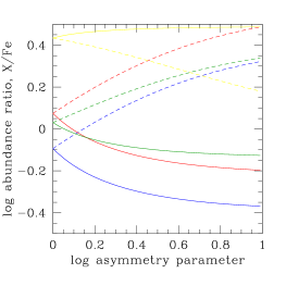
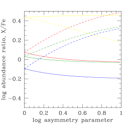
Figure 2.— Left panel (a): ICM (solid lines) and stellar (broken lines) abundance ratios with respect to Fe for O (red), Mg (blue), Si (green), and Ni (yellow) versus $\alpha^{SN}$ for the standard $\beta^{cc}=0.6$. Right panel (b): same as (a) for $\beta^{cc}=0.3$.

The effects on cluster enrichment of adopting different SNIa yield sets is shown in Figures 3-5. The solid lines correspond to previous plots that utilize Kobayashi et al. (2006) yields, the dotted lines use the same SNcc yields, but alternative SNIa yield sets from Nomoto et al. (1997); Maeda et al. (2010) – see Loewenstein & Davis (2010). Here we focus on Fe, Ni, and Si (O and Mg are always dominated by SNcc enrichment and insensitive to this choice). Figure 3 shows the total baryon enrichment, which is independent of $\beta^{cc}$ and $\alpha^{SN}$, and demonstrates that star formation efficiencies $\varepsilon_{sf}\sim 0.25-0.5$ are required to enrich cluster baryons to a relatively modest Fe abundance of half-solar – $\varepsilon_{sf}\sim 0.4-0.7$ to attain 0.75 solar. Figures 4 and 5 that, respectively, show the ICM abundances for the standard lock-up parameters, and the maximum ICM abundances corresponding to zero stellar metallicity, demonstrate that the conclusions about the required efficiency of star formation are not a result of a particular choice of yields sets. Using SNcc yields from Woosley & Weaver (1995) (their standard explosion energy, solar abundance progenitor model) does not alter these conclusions.

Figure 3.— Left panel (a): Average Fe abundance of all cluster baryons (stars and gas) as a function of star formation efficiency, $\varepsilon_{sf}$, assuming a single SNcc yield set but a wide range of SNIa yield sets (see text for details). The horizontal dotted line shows the very conservative value of $Z_{Fe,bar}=0.5$. Middle panel (b): Same as (a) for Ni. Right panel (c): Same as (a) for Si.

Figure 4.— Same as Figure 3 for ICM abundance, assuming the standard $\beta^{cc}=0.6$, $\alpha^{SN}=2$.

Figure 5.— Same as Figure 3 for the maximum ICM abundance, i.e. $\beta^{cc}=0$.

From the results in this section, we confirm that ICM Fe abundances cannot be produced if $\varepsilon_{sf}\sim 0.15$ ($f_{*}/f_{ICM}\sim 0.11$) and quantified the shortfall as a function of how efficiently metals in general, and SNIa products in particular, are locked up in stars. For $\varepsilon_{sf}\sim 0.3$ ($f_{*}/f_{ICM}\sim 0.24$), they can – but only for small lock-up fractions such that $\sim 85$% of SNIa, and $\sim 70$% of SNcc, metal production is embedded in the ICM and (by implication) $Z_{Fe,*}\sim 0.5$. The assumption of a standard IMF is adopted throughout this section, an assumption we relax in the following section.

4. A More Comprehensive Examination (II): Effects of Changing the IMF

The initial mass function (IMF) of stars in cluster galaxies and intracluster space is intimately connected to estimates of ICM enrichment, impacting the mass in stars calculated from the total light, the mass return fraction (or, equivalently, the ratio of current stellar mass to mass converted into stars), and the numbers of SNcc and SNIa explosions expected per mass formed into stars. The general characteristics of the IMF in various Milky Way sub-populations are now well-determined and generally mutually consistent (Bastian et al., 2010). Although several functional forms are commonly used for the “canonical” IMF (Kroupa et al., 2012), these must share the properties of a Salpeter-like slope at high mass with a break to a flatter slope below $\sim 0.5-1~{}{\mathrm{M}}_{\sun}$. Many of the best-studied environments are consistent with the hypothesis that this form is “universal” in space and time, but variations in extreme star forming environments that predominate in the early universe (when most stars in the elliptical galaxies that dominate the stellar content in clusters form) may explain a number of anomalies, such as an apparent inconsistency between the observed evolution of the global star formation rate and stellar mass densities (Narayanan & Davé 2012a, and references therein).

Several recent observational investigations of elliptical galaxies find direct evidence in the mass-to-light ratio for either an excess of stellar remnants as realized in a “top-heavy” IMF; or, of low mass stars as realized for a “bottom-heavy” IMF (e.g., Cappellari et al. 2012; see Section 5 below). By exploiting the level and pattern of ICM abundances we constrain the properties of the enriching stellar population. We may then exclude particular elliptical galaxy IMFs under the parsimonious assumption that these optically studied stars originate from the same parent IMF as those that enrich the ICM – or, alternatively, call this assumption into question.

4.1. Models and Parameters

Simply put, the level of metal enrichment of the stellar and ICM baryonic sub-components in clusters is a reflection of their respective total masses, the total numbers of SNIa and SNcc that enrich each constituent, and the nucleosynthetic yields of each of these supernova explosion types. In previous sections, these are expressed in terms of the mass return fraction, $r_{*}$, and formation efficiency, $\varepsilon_{sf}$ of the stars, the total and relative numbers of SNIa and SNcc per star formed ($\eta^{Ia}$, $R^{SN}$), and phenomenological supernova lock-up and asymmetry parameters ($\beta^{cc}$ and $\alpha^{SN}$) characterizing the ultimate destination (ICM or stars) of supernova products. In Appendix A these are further deconstructed into more fundamental astrophysical functions and parameters directly connected to stellar and galaxy evolution, thus providing a self-consistent astrophysical framework for understanding the effect of varying the IMF on cluster enrichment. Ultimately these are reduced to the following: (1) The functional form of the IMF (see below); (2) the present-day main sequence turnoff mass ($0.9~{}{\mathrm{M}}_{\sun}$); (3) the remnant-progenitor mass relationships for ($<8~{}{\mathrm{M}}_{\sun}$) intermediate- (equation A4) and ($\geq 8~{}{\mathrm{M}}_{\sun}$) high-mass (equation A29) stars derived, for the former, from well-established standard white dwarf masses and, for the latter, from a model for the evolution of the stellar population and the delayed-explosion compact remnant prescription in Fryer et al. (2012); (4) the ratio of mass ejected from galaxies into the ICM during star formation to the mass of stars formed, $\delta_{GW}$; (5) the galaxy formation efficiency, $\varepsilon_{gal}$; and, (5) various supernovae switches and parameters that we now describe. For SNcc we assume progenitor masses from $m_{cc}=8~{}{\mathrm{M}}_{\sun}$ to $m_{up}$, where $m_{up}$ may differ from the IMF upper mass limit $m_{hi}$ (but is the same by default, and assumed so in calculating the high mass return fraction). Since we adopt the IMF-averaged SNcc yields of Kobayashi et al. (2006) as a function of progenitor metallicity $Z_{cc}$, $Z_{cc}$ must be specified as well. For SNIa we consider the yield sets described in Section 3, assume progenitors in the $3-8~{}{\mathrm{M}}_{\sun}$ range, and must specify the efficiency $\varepsilon^{Ia}$ defined as the fraction of $3-8~{}{\mathrm{M}}_{\sun}$ that result in SNIa. In addition, the “prompt” fraction of SNIa that explode during the star formation epoch and so may be incorporated into stars or ICM, $f^{Ia}_{p}$, (while a fraction $1-f^{Ia}_{p}$ strictly enrich the ICM) must be specified.

Our default IMF is the Kroupa et al. (2012) segmented power-law with slopes and mass scales that can explain local star formation (Appendix A); other defaults are $Z_{cc}=1$, W7 yields, $\varepsilon_{gal}=0.25$ and $\delta_{GW}=0.5$ ($\varepsilon_{sf}=0.17$, $f_{*}/f_{ICM}\sim 0.11$), $\varepsilon^{Ia}=0.076$ (Section A.2), and $f^{Ia}_{p}=0.5$. Under these conditions, $r_{*}=0.41$ ($r^{im}_{*}=0.25$, $r^{hi}_{*}=0.16$ for intermediate- and high- mass stars, as delineated above) while the fraction in stellar remnants is 0.17 (0.11/0.06 from intermediate/high-mass stars), $\eta^{cc}=0.011$, $\eta^{Ia}=0.0022$, $\alpha^{SN}=2$ and $\beta^{cc}=0.39$ – similar to the default parameters in Section 3. The resulting abundances are shown in Table 1 where, once again as expected, we find reasonable stellar abundances but ICM abundances too low by a factor of $\sim 2$. For comparison we also display the abundances for a Salpeter IMF, which fails to provide sufficient metals for all components (including stars) for this default set of parameters.

Table 1ICM Abundances from Default Parameters

	0	Mg	Si	Fe	Ni
Baryons	0.44 (0.27)	0.30 (0.18)	0.38 (0.23)	0.32 (0.20)	0.84 (0.53)
Stars	1.74 (1.05)	1.19 (0.72)	1.35 (0.82)	0.87 (0.54)	1.90 (1.21)
ICM	0.30 (0.15)	0.20 (0.10)	0.27 (0.15)	0.26 (0.15)	0.72 (0.43)

Note. — All abundances relative to (Asplund et al., 2009) solar standard. The values in parentheses are for a Salpeter IMF with the default values of $\varepsilon_{gal}$, $\delta_{GW}$, $\varepsilon^{Ia}$, and $f^{Ia}_{p}$, and the same range of masses ($0.07-150~{}{\mathrm{M}}_{\sun}$).

Table 2Model IMF Parameters

	$m_{lo}$	$m_{br}$	$\alpha_{lo}$	$\alpha_{hi}$
sl-0	0.07	$\cdots$	$1.8\rightarrow 2.3$	$=\alpha_{lo}$
sl-1	0.07	0.5	$0.3\rightarrow 2.4$	2.3
sl-2	0.07	1.0	$0.3\rightarrow 2.3$	2.3
sl-3	0.07	0.5	1.3	$1.8\rightarrow 2.5$
sl-4	0.07	1.0	1.3	$1.8\rightarrow 2.5$
sl-5	0.07	8.0	1.3	$1.5\rightarrow 3.3$
m-1	$0.01\rightarrow 1.0$	1.0	1.3	2.3
m-2	$0.01\rightarrow 0.5$	0.5	1.3	2.3
m-3	$0.07$	$0.5\rightarrow 5.45$	1.3	2.3

Note. — $m_{hi}=150~{}{\mathrm{M}}_{\sun}$ for all models displayed here. $m_{br}$ – equivalent to $m2=0.5~{}{\mathrm{M}}_{\sun}$ for models sl-1, sl-3, and m-2; and $m_{3}$ (default: $1~{}{\mathrm{M}}_{\sun}$) for models sl-2, sl-4, sl-5, m-1, and m-3 – is defined as the mass where the IMF slope transitions to its high-mass value. Models sl-4 and sl-5 include an additional break from $\alpha_{1}=1.3$ to $\alpha_{2}=2.3$ at $m_{2}$. $\alpha_{1}=\alpha_{lo}$ and $\alpha_{3}=\alpha_{hi}$, while $\alpha_{2}=\alpha_{lo}$ for models sl-2, m-1, and m-3; $\alpha_{2}=\alpha_{3}$ for models sl-1, sl-3, m-2; and, is set at the default $\alpha_{2}=2.3$ for models sl-1, sl-4, sl-5, and m-2. Parameter ranges correspond to those with physical solutions; i.e., $f^{Ia}_{p}$ and $\delta_{GW}>0$ and $\varepsilon_{gal}<1$ – for the sl-4 model with higher SNIa efficiency (star-to-gas ratio) the range shifts to $1.5\rightarrow 2.5$ ($2\rightarrow 2.5$); see below and Tables 3 and 4.

Our approach to examining the effects of varying the IMF on ICM enrichment, that attempts to make comparisons at fixed values of the observables to the extent possible, is as follows. As detailed in Appendix A, we consider departures from the “canonical” IMF (Table 2) described according to sequences with either a single slope below the break mass $m_{3}$, or an additional distinct slope below 0.5 ${\mathrm{M}}_{\sun}$. Either the lower mass limit ($m_{lo}$), or the slopes ($\alpha_{1}$ or $\alpha_{3}$) at low or high mass ends may be varied. Additionally, $m_{3}$ may vary in sequences of the first type. To isolate the effect of the IMF on ICM abundances, we impose invariance on the stellar Fe and O abundances (Table 1). This determines the necessary adjustments in the parameters $\delta_{GW}$ and $f^{Ia}_{p}$ (for some $\varepsilon^{Ia}$). For fixed yield sets, invariance in $Z_{Fe,*}$ and $Z_{O,*}$ assures invariance in all stellar abundances. Finally, we consider these variations at fixed present-day baryon inventory (11% stars, 89% ICM), which is equivalent to adjusting $\varepsilon_{gal}$ so as to maintain constant $\varepsilon_{sf}(1-r_{*})$ (equations 2, A26) – thus enabling us to investigate what adjustments in IMF (if any) may explain observed ICM abundances assuming this nominal star-to-gas ratio. The imposition of these constraints rule out those IMFs that imply unphysical values of $\delta_{GW}$($<0$), $f^{Ia}_{p}$($>1$), or $\varepsilon_{gal}$($>1$) – i.e., some IMFs are incompatible with observed stellar abundances and a $\sim$9:1 ratio of ICM to stars (thus the limited range of the variable IMF parameters in Table 2).

4.2. Impact of Varying the IMF

We remind the reader that our standard IMF has slope $\alpha=1.3$ below 0.5 ${\mathrm{M}}_{\sun}$, and 2.3 above. Figures 6a-d show the impact on ICM enrichment of varying one (and only one) of the slopes and (in some cases) adjusting the break mass, by plotting the Fe abundance and Mg/Fe, Si/Fe, and Ni/Fe ratios versus the deviation in the non-fixed slope from these standard values. This covers many of the IMFs considered in the literature as possibly resolving various conflicts between expectations and observations of stellar populations in elliptical and/or starburst galaxies. For models sl-1 (sl-2) $\alpha$ below 0.5 ${\mathrm{M}}_{\sun}$ (1 ${\mathrm{M}}_{\sun}$) is varied with $\alpha$ above these single break masses fixed at 2.3 – i.e. positive (negative) $\Delta\alpha$ corresponds to bottom-heavy (-light) IMFs. For models sl-3, sl-4, and sl-5, $\alpha$ is varied above break masses of 0.5 ${\mathrm{M}}_{\sun}$, 1 ${\mathrm{M}}_{\sun}$, and 8 ${\mathrm{M}}_{\sun}$, respectively, with $\alpha=2.3$ between 0.5 ${\mathrm{M}}_{\sun}$ and the break mass in the latter two. For these models, positive (negative) $\Delta\alpha$ corresponds to top-light (-heavy) IMFs. In addition, we plot the results for a single-slope IMF (sl-0). We can see that $Z_{Fe,ICM}\sim 0.5$ is predicted for either a (1) bottom-light IMF with $\alpha(\leq 1{\mathrm{M}}_{\sun})\sim 1$, (2) top-heavy IMF with $\alpha(>0.5{\mathrm{M}}_{\sun})\sim 2$ or $\alpha(>1{\mathrm{M}}_{\sun})\sim 1.8$, (3) single-slope IMF (i.e. both bottom- and top-heavy) with $\alpha\sim 1.8$. As expected, $Z_{Fe,ICM}\sim 0.1$ for the pure Salpeter IMF (single slope and bottom-light cases with slope 2.35).

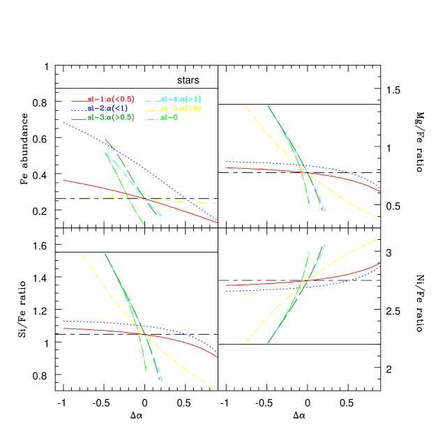
Figure 6.— Clockwise from upper left (a)-(d): ICM Fe abundance and Mg/Fe, Ni/Fe, and Si/Fe abundance ratios for models with departures, with respect to the standard IMF, in either high- or low-mass slope: $\Delta\alpha=\alpha_{hi}-2.3$ for top-heavy/light (sl-1, sl-2) and $\alpha_{lo}-1.3$ for bottom-light/heavy (sl-3, sl-4 , sl-4), models – see text and Table 2 for details. Curves for models sl-3 and sl-4 closely trace each other in the ratio plots. The solid and broken horizontal lines, respectively, show the stellar, and standard model ICM, values (Table 1).

Varying the lower mass cutoff provides an alternative means of producing either bottom-heavy ($m_{lo}<0.07~{}{\mathrm{M}}_{\sun}$) or bottom-light ($m_{lo}>0.07~{}{\mathrm{M}}_{\sun}$) IMFs, while increasing the break mass that delineates $\alpha=1.3$ from $\alpha=2.3$ (Narayanan & Davé, 2012a) is also bottom light in the sense that the fraction of low-mass stars relative to those at intermediate and high mass is suppressed. As shown in Figure 7a, these alternatives can explain $Z_{Fe,ICM}=0.5$ for IMFs with the standard high mass slope $\alpha=2.3$ if the IMF lower mass cutoff is shifted from the standard $m_{lo}=0.07~{}{\mathrm{M}}_{\sun}$ to $m_{lo}\sim 0.2~{}{\mathrm{M}}_{\sun}$ for an IMF with a single break at 1 ${\mathrm{M}}_{\sun}$, what is (essentially) a Salpeter IMF with $m_{lo}\sim 0.5~{}{\mathrm{M}}_{\sun}$, or for an IMF with the break between $\alpha=1.3$ and $\alpha=2.3$ shifted from 0.5 to $\sim 1~{}{\mathrm{M}}_{\sun}$. The last would seem to represent a particularly modest departure from the standard IMF.

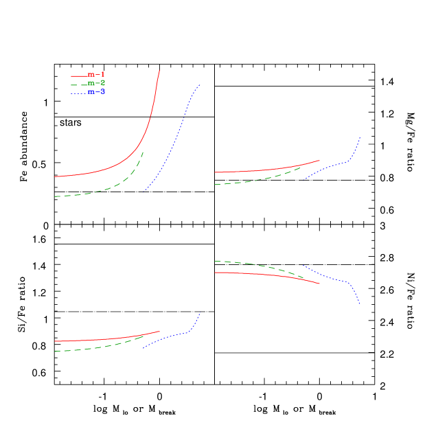
Figure 7.— Same as figure 6 for departures, with respect to the standard IMF, in lower mass limit or break mass – see text and Table 2 for details.

Bottom-light and top-heavy scenarios may be directly distinguished in ICM spectra via abundance ratios, as demonstrated in Figures 6b-d, 7b-d, and 8a-c; and Table 3. These essentially define two branches in the $Z_{Fe,ICM}-(\alpha/Fe)_{ICM}$ plane (Figure 8), with ratios in the top-heavy branch connecting to the stellar ratio as the IMF flattens (and $f^{Ia}_{p}\rightarrow 1$), and abundances for the bottom-light IMFs (assured to have $f^{Ia}_{p}=0.5$) universally rising in lockstep with the elimination of low-mass stars. Table 3, confined to those models that predict $Z_{Fe,ICM}=0.5$, illustrates how the $\alpha/Fe_{Fe,ICM}$ ratios might be exploited to distinguish among bottom-light and top-heavy IMF explanations for ICM enrichment – for the former, ratios deviate more strongly from those in stars (smaller $\alpha/Fe_{Fe,ICM}$, larger Ni/Fe) and provide a better match to the data (Simionescu et al., 2009).

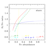
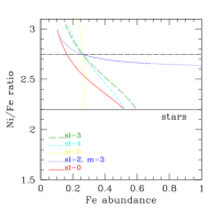
Figure 8.— ICM abundance ratios, with respect to Fe, for Mg – left panel (a), Si – middle panel (b), and Ni – right panel (c) – vs. Fe abundance for top-heavy models sl-0, sl-3, sl-4, and sl-5; and, for bottom-light models sl-2 and m-3 (all bottom-light models considered essentially follow the same curve).

Table 3Abundance Ratios in Models with $Z_{Fe,ICM}=0.5$

		$O/Fe$	$Mg/Fe$	$Si/Fe$	$Ni/Fe$
stars	$\cdots$	2.0	1.4	1.6	2.2
salpeter	$\cdots$	1.0	0.68	0.97	2.8
canonical	$\cdots$	1.1	0.77	1.0	2.7
sl-0	$\alpha=1.83$	1.9	1.3	1.5	2.2
sl-2	$\alpha_{lo}=1.06$	1.2	0.85	1.1	2.7
sl-3	$\alpha_{hi}=1.97$	1.7	1.2	1.4	2.4
($\varepsilon^{Ia}=0.13$)	$\alpha_{hi}=2.22$	0.85	0.57	0.87	2.9
(star/gas=0.25)	$\alpha_{hi}=2.36$	1.0	0.69	0.97	2.8
sl-4	$\alpha_{hi}=1.85$	1.9	1.3	1.5	2.3
m-1	$m_{lo}=0.20$	1.2	0.85	1.1	2.7
m-2	$m_{lo}=0.42$	1.2	0.85	1.1	2.7
m-3	$m_{br}=1.25$	1.2	0.85	1.1	2.7

Note. — Canonical and Salpeter model ratios, and stellar ratios, included for comparison purposes; $\varepsilon^{Ia}=0.13$ and star/gas=0.25 variations of model sl-3 also included.

4.3. Implications of Models with Nonstandard IMFs

Table 4 displays the essential characteristics of models that produce $Z_{Fe,ICM}=0.5$, and are constrained to match the standard values of stellar metallicity and $f_{*}/f_{ICM}$. Several general properties, as well as others that distinguish top-heavy from bottom-light solutions emerge. Relative to the model with canonical IMF, all have a relative deficiency of unevolved low-mass stars, and hence $\sim 30$% higher mass return ($r_{*}$) and remnant ($f_{rem}$) fractions – implying $\sim 30$% upward adjustments in the integrated mass of stars formed based on the present-day mass, and $\sim 60$% upward adjustments based on the luminous stellar mass. The “extra” metals are explained by a larger fraction of stars in the supernova-progenitor mass range, and a larger ratio of mass in stars formed to present-day stellar mass.

Successful top-heavy models are characterized by a large “prompt” fraction of SNIa and prodigious galactic winds, and have low lock-up fraction and modest asymmetry between stellar and ICM abundance patterns. That is, the extra ICM metals are mostly associated with the rapid early star formation epoch where both formation of SNcc and SNIa progenitors, and delivery of the metals from star forming sites to extragalactic hot gas, are efficiently realized.

Successful bottom-light models are characterized by the standard prompt SNIa fraction and more modest (though still substantial) galactic winds, with a larger fraction of ICM enrichment occurring during the passive, post-star-formation phase. In these models, the implied fraction of mass originally in galaxies is 0.42 and the fraction of the ICM that is primordial, $f_{prim}=0.65$ – compared to 0.25 and 0.83 in the canonical model. For the top-heavy models these take on more extreme values – each on the order 0.5 – although, due to the effects of galactic winds, the star formation efficiencies are not appreciably different.

The different abundance patterns predicted in bottom-light and top-heavy models is reflected in values of $R^{SN}_{ICM}$ that are $\sim$twice as high for the former, more consistent with – though still lower than – the value recently inferred by (Bulbul et al., 2012) for the central region in Abell 3112.

Table 4Characteristics of Models with $Z_{Fe,ICM}=0.5$

		$r_{*}$	$f_{rem}$	$f^{Ia}_{p}$	$\delta_{GW}$	$\varepsilon_{gal}$	$\varepsilon_{sf}$	$\eta^{Ia}$	$\eta^{cc}$	$\beta^{cc}$	$\alpha^{SN}$	$R^{SN}_{ICM}$	$f_{prim}$
salpeter	$\cdots$	0.27	0.11	0.5	0.5	0.25	0.17	0.0014	0.0065	0.50	2.0	0.32	0.86
canonical	$\cdots$	0.41	0.17	0.5	0.5	0.25	0.17	0.0022	0.011	0.39	2.0	0.27	0.83
sl-0	$\alpha=1.83$	0.56	0.24	0.96	1.7	0.60	0.22	0.0020	0.019	0.16	1.0	0.11	0.44
sl-2	$\alpha_{lo}=1.06$	0.54	0.22	0.5	0.97	0.42	0.21	0.0028	0.014	0.24	2.0	0.23	0.65
sl-3	$\alpha_{hi}=1.97$	0.54	0.23	0.78	1.5	0.54	0.22	0.0023	0.018	0.18	1.3	0.13	0.50
($\varepsilon^{Ia}=0.13$)	$\alpha_{hi}=2.22$	0.45	0.18	0.33	0.75	0.31	0.17	0.0039	0.013	0.32	3.1	0.40	0.76
(star/gas=0.25)	$\alpha_{hi}=2.36$	0.38	0.16	0.46	0.33	0.43	0.32	0.0021	0.0096	0.46	2.2	0.32	0.72
sl-4	$\alpha_{hi}=1.85$	0.55	0.24	0.93	1.7	0.59	0.22	0.0021	0.019	0.17	1.1	0.11	0.45
m-1	$m_{lo}=0.20$	0.54	0.22	0.5	0.97	0.42	0.21	0.0028	0.014	0.24	2.0	0.23	0.65
m-2	$m_{lo}=0.43$	0.54	0.22	0.5	0.98	0.42	0.21	0.0028	0.014	0.23	2.0	0.23	0.64
m-3	$m_{br}=1.25$	0.53	0.22	0.5	0.98	0.42	0.21	0.0029	0.014	0.23	2.0	0.23	0.64

Note. — Canonical and Salpeter models included for comparison purposes; $\varepsilon^{Ia}=0.13$ and star/gas=0.25 variations of model sl-3 also included.

4.4. Other Variations

4.4.1 Supernova Yields

In most cases, varying the SNIa yield set primarily affects the predicted (stellar and ICM) Ni/Fe ratios – which are not well-determined in clusters at this time. Exceptions are yield sets with particularly low ($<0.4~{}{\mathrm{M}}_{\sun}$) Fe yields, i.e. the C-DEF and C-DDT in Maeda et al. (2010). These models cannot self-consistently produce the observed stellar abundances and $Z_{Fe,ICM}=0.5$. Since there is a narrow range of Fe yields in SNcc calculations, our results are insensitive to the choice of $Z_{cc}$ – though, in principle, abundance ratios among $\alpha$-elements could carry SNcc yield diagnostic information. Decreasing the SNcc upper mass limit, $m_{up}$, with respect to the IMF upper limit, $m_{hi}$, lowers the predicted metallicities – though the effect is small unless the upper mass IMF slope is very flat.

Overall our models are conservative in the sense of maximizing Fe yields by adopting high values for the SNIa Fe yield ($0.74~{}{\mathrm{M}}_{\sun}$), and for $m_{hi}$ ($150~{}{\mathrm{M}}_{\sun}$).

4.4.2 SNIa Efficiency

Maoz & Mannucci (2012) estimated that a $1.7\times$ higher Type Ia supernova rate per unit mass of star formed is implied by the ICM Fe abundances for otherwise standard assumptions. We construct a scenario along these lines by considering an increase in $\varepsilon^{Ia}$ – the fraction of $3-8~{}{\mathrm{M}}_{\sun}$ that explode as SNIa – from 0.076 to 0.13 (${f_{*}}/{f_{ICM}}$ and stellar abundances constrained to match the standard values; Section 4.1). Indeed we find $Z_{Fe,ICM}=0.5$ for an IMF that otherwise (i.e., in terms of IMF, star formation efficiency, SNcc lock-up fraction and rate, and ICM primordial fraction) approximates the standard model (Tables 3 and 4). Naturally, the increase in efficiency of formation of SNIa progenitors results in a large asymmetry between the stellar and ICM abundance patterns ($\alpha^{SN}=3.1$), as reflected in the more nearly solar $[\alpha/Fe]_{ICM}$ ratio and consistent with ICM abundance patterns ($R^{SN}_{ICM}=0.4$; Bulbul et al. (2012)) – see Tables 3 and 4, and Figures 9 and 10 that display results for such a variation of model sl-3. If this is the correct explanation for the observed ICM abundances, one must seek an astrophysical explanation for boosting $\varepsilon^{Ia}$ in rapidly star-forming systems.

4.4.3 Star-to-ICM Ratio

As briefly discussed in Section 2.2, the present-day star-to-ICM ratio may exceed our standard value of 11%, e.g. due to an unaccounted-for ICL fraction or underestimate of the stellar mass-to-light ratio. If we increase ${f_{*}}/{f_{ICM}}$ from 0.11 to 0.25, a generally satisfactory resolution of the cluster elemental abundance paradox is achieved – a level of Fe enrichment and abundance pattern ($R^{SN}_{ICM}=0.32$) consistent with observations is attained for an IMF and other parameters in line with expected values – with the notable exception of the increase in star efficiency to $\varepsilon_{sf}=32$% – see Tables 3 and 4. The results of this variation on model sl-3 are also displayed Figures 9 and 10. It is worth pointing out at this juncture that we defined $\varepsilon_{sf}$ as the fraction of cluster baryons that form stars; in our models the fraction of galactic baryons that form stars (where “galaxies” are defined as locations where stars form and eject mass into the ICM) is $\varepsilon_{sf}/\varepsilon_{gal}=(1+\delta_{GW})^{-1}$ – 75% for this ${f_{*}}/{f_{ICM}}=0.25$ model, but also 2/3 for the standard model.

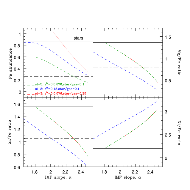
Figure 9.— ICM Fe abundance and Mg/Fe, Ni/Fe, and Si/Fe abundance ratios versus slope above $0.5~{}{\mathrm{M}}_{\sun}$ (assuming slope 1.3 for $m<1~{}{\mathrm{M}}_{\sun}$) – i.e., model sl-3, for boosted SNIa progenitor formation efficiency ($\varepsilon^{Ia}$) or star-to-ICM ratio (${f_{*}}/{f_{ICM}}$). As for all models, stellar abundances (solid horizontal lines) are fixed at their standard values (Table 1). Results for a standard IMF (broken horizontal lines), and for model sl-3 with standard $\varepsilon^{Ia}$ and ${f_{*}}/{f_{ICM}}$, are reproduced.

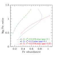
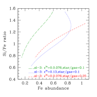
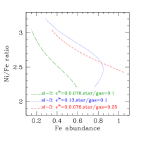
Figure 10.— ICM abundance ratios with respect to Fe for Mg – left panel (a), Si – middle panel (b), and Ni – right panel (c) – vs. Fe abundance for model sl-3 and its boosted $\varepsilon^{Ia}$ and star-to-ICM ratio counterparts.

5. Summary and Discussion

Star formation, with a canonical IMF and standard efficiency in producing SNIa, that builds up a stellar population comprising $\sim 10$% of the current overall cluster baryon content falls short by a factor of $>2$ of explaining a typical rich cluster half-solar ICM Fe abundance (Sections 2.3-2.4). This is the case even if predicted ICM abundances are enhanced by increasing the efficiency at which metals are ejected from galaxies (and where, as a result, the overall abundance in stars is significantly below solar), unless the conversion efficiency of cluster baryons into stars is also increased well above 10% (Section 3).

Section 4 (and Appendix A) constructs and utilizes a phenomenological model for the evolution of an old, simple stellar population to quantify the changes in the IMF shape (high and low mass slopes, break mass) from its standard form required to bring the ICM metallicity and cluster stars into concordance in the sense that they be consistent with the same parent star formation history. The necessary departure may be either in the “bottom-light” or “top-heavy” sense, with the former tentatively preferred based on better agreement with observed ICM abundance patterns and on a higher primordial ICM fraction. It is further demonstrated that if a standard IMF is to be preserved, a boost in the efficiency of forming stars from gas well beyond that consistent with a gas-to-star ratio of 10, and/or of producing SNIa progenitor systems, is required. These calculations are conservative in the sense of maximizing the enrichment of the stellar population through the choice of SN parameters (e.g., SNIa Fe yields, the upper mass limit for SNcc).

Stars born in cluster potential wells (or those of their progenitors) must be responsible for the high level of enrichment measured in the ICM; however, there is increasing tension between this truism and the parsimonious assumption that the stars in the generally old populations studied optically emerged from the same formation sites during the same epochs. Quantifying this tension, and bolstering the case against the universality of star formation are the two primary implications of this study. In the remainder of this section we elaborate on these themes.

5.1. The ICM-Enriching Stellar Population as Distinct from that Observed in Elliptical Galaxies

In some cases the departure from the canonical IMF is modest – a shift of a few tenths in the slope over some mass range or an increase in the mass at which the slope steepens from 0.5 to $1.25~{}{\mathrm{M}}_{\sun}$. However, optical determinations of the IMF from kinematic and population studies in elliptical galaxies are trending in the opposite direction (Treu et al., 2010; Auger et al., 2010; van Dokkum & Conroy, 2010, 2011, 2012; Conroy & van Dokkum, 2012; Thomas et al., 2011; Dutton et al., 2012; Smith et al., 2012; Cappellari et al., 2013; Tortora et al., 2012; Spiniello et al., 2011, 2012; Ferreras et al., 2013; Sonnenfeld et al., 2012; Goudfrooij & Kruijssen, 2013; Dutton et al., 2013; Dutton & Treu, 2013). The kinematic evidence that indicates a larger mass-to-light ratio in massive ellipticals than expected based on a standard IMF is consistent with either an IMF that is top-heavy and so produces more stellar remnants, or one that is bottom heavy and produces more unevolved low mass stars. However population synthesis modeling of elliptical galaxy spectra favor the latter, and a consensus appears to be emerging for an IMF that is bottom-heavy in elliptical galaxies with central velocity dispersions $>150$ km s^-1 where most of the present-day stellar mass in galaxy clusters reside, being at least as steep as a Salpeter IMF if characterized by a single slope (and steeper still at the highest galaxy masses). The apparent dependence of the IMF on elliptical galaxy mass is strong evidence against the existence of a universal IMF.

The chasm between the amount of metals expected to be produced from a stellar population with such a steep IMF, and the observed level of cluster enrichment is illustrated in the plots of Fe abundance in the ICM versus cluster star-to-gas ratio for three distinct IMFs in Figure 11. Standard yield sets and values of the parameters $\delta_{GW}$ (0.5), $f^{Ia}_{p}$ (0.5), and $\varepsilon^{Ia}$ (0.076) are assumed (Section 4.1). Also plotted are the overall averaged Fe abundances for the total cluster baryons; these are independent of the detailed galaxy evolution parameters $\delta_{GW}$ and $f^{Ia}_{p}$. As might easily be inferred from previous considerations, it is clear that the model with Salpeter IMF requires an excessively large gas-to-star ratio, and that an IMF as steep as $\phi\sim m^{-3.05}$ unequivocally falls short by more than an order of magnitude of producing the required amount of metals.

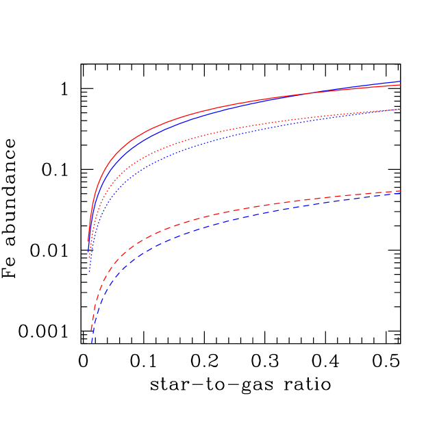
Figure 11.— Fe abundance in the ICM (blue curves) and, overall, in cluster baryons (red curves) for the following three IMFs: (solid curves) standard (Kroupa et al., 2012), (dotted curves) single slope with $\phi\sim m^{-2.35}$ (Salpeter, 1955), (dashed curves) single slope with $\phi\sim m^{-3.05}$.

The most straightforward explanation for reconciling the steep IMFs based on optical spectroscopic studies of elliptical galaxies and the relatively flat IMFs needed to produce the cluster metals is to reject the conventional wisdom that the stellar populations in ellipticals that dominate the cluster stellar mass are primarily responsible for ICM enrichment. Such a decoupling begs the question of the origin and present-day whereabouts of the ICM-enriching stars and motivates consideration of scenarios with pre-enrichment (that would presumably be accompanied by pre-heating) in protocluster environments by a currently inconspicuous stellar population. The independence of the enriching population of high mass stars from present-day galaxies is supported by the remarkably small range of cluster metallicities (Baldi et al., 2012) as compared with the large variation in inferred stellar mass fraction – and the lack of correlation between the two (Bregman et al., 2010).

However, an important caveat with respect to the optical spectroscopic studies is their general confinement to regions well inside the half-light radius as well as systems at low redshift. Given the emerging paradigm of the multi-stage, inside-out formation/assembly/growth of ellipticals by multiple mechanisms (star-forming major mergers, “dry” minor mergers, and cold and hot gas accretion; e.g., Conselice et al. 2013, Patel et al. 2013, Huang et al. 2013), spatial gradients and temporal evolution in properties of elliptical galaxy stellar populations such as the IMF is to be expected (La Barbera et al., 2012). With the current dearth of global constraints, as well as degeneracies between the inferred dark matter content and the IMF (Wegner et al., 2012; Tortora et al., 2013) and possible systematic errors resulting from nonsolar abundance ratios (Ferreras et al., 2013), an IMF in cluster ellipticals that is flatter than currently inferred in the core when integrated over space and time is plausible (Davé, 2008; Worthey, Ingermann, & Serven, 2011; Narayanan & Davé, 2012b).

Recent arguments for a reconsideration of bimodal star formation – hints for an IMF that is top-heavy in older, but bottom-heavy in younger, star clusters (Zaritsky et al., 2012, 2013), or top-heavy in denser environments (Marks et al., 2012) – support this. The evolution in the cluster star formation environment plausibly leads to an IMF in elliptical galaxies (and their progenitors) that transition from one initially weighted towards the mass range that includes SNcc and (prompt) SNIa progenitors to one especially conducive to low mass star formation at later times (Narayanan & Davé(2012ab; see, also Suda et al. 2013). We note that the high metallicities seen in the gas in high redshift quasar hosts (Dietrich et al., 2003a, b) also indicate an early epoch of rapid star formation that efficiently produces SN progenitors and is accompanied by powerful galactic outflows (Di Matteo et al., 2004; Wang et al., 2002).

5.2. The Enriching Stellar Population as Distinct from that Observed in our Galaxy

The hypothesis that star formation is universal is refuted by analysis of the level and pattern of ICM elemental abundances. The star formation characteristics of the stellar population responsible for these metals must depart from that studied locally in one or more of the following ways: (1) engender a higher fraction of high mass stars, (2) more efficiently form stars from gas, (3) more efficiently produce SNIa progenitor systems. In addition, we saw in the previous subsection that the IMF if the enriching population is distinct from that recently inferred in the central regions of elliptical galaxies. Arguments for (1) were presented above. We now examine the feasibility, and implications, of hypotheses (2) and (3).

The true star-to-gas ratio (and implied star formation efficiency) remains uncertain, with stellar masses difficult to estimate given low surface brightness extended light and the likelihood of multiple stellar populations that complicate the conversion from measured light in some aperture to total stellar mass (Munshi et al., 2013; Mitchell et al., 2013). The ICL contribution is also uncertain – although recent measurements for those most massive clusters that concern this work indicate modest ICL mass fractions (Krick & Bernstein, 2007; Sanderson et al., 2013). Both bottom-heavy as now being inferred in elliptical cores, and top-heavy/bottom-light as required by ICM enrichment, IMFs may result in upward revisions in mass-to-light ratios. A global value of $f_{*}/f_{ICM}\geq 0.25$, even for rich clusters, does not seem to be excluded by observations at this time. The star formation efficiency corresponding to $f_{*}/f_{ICM}\geq 0.25$, excluding the primordial portion of the ICM that does not engage in star formation (see Section 4.4.3, above), is $\{5\varepsilon_{gal}(1-r_{*})\}^{-1}$, where $\varepsilon_{gal}$ (first defined in Appendix A) is the fraction of baryons initially in star-forming structures. This quantity has an absolute minimum of 0.2, is $>0.3$ for any reasonable value of the mass return fraction $r_{*}>1/3$, and $>0.5$ for $r_{*}>1/3$ and $\varepsilon_{gal}<0.6$. These considerations indicate that a substantial fraction of protocluster gas was in the form of dense star-forming protogalaxies or pre-galactic fragments. There are clearly profound implications for such a high stellar fraction and star formation efficiency for evaluating the magnitude – and perhaps even the reality – of the “overcooling” problem (McCarthy et al., 2011) and the physics of star formation quenching as it pertains to the cluster environment, as well as for the precision in using cluster gas fractions – that must be converted to baryon fractions using a correction for stellar content – to constrain the cosmological world model (Allen et al., 2008).

Given the uncertainty in the nature and possible diversity of SNIa progenitors, and the difficulties in reproducing observed rates (e.g., Toonen et al. 2012, Quimby et al. 2012, and references therein), the feasibility of an efficiency of SNIa progenitor formation in galaxy clusters that exceeds the standard $\varepsilon^{Ia}=0.076$ is not easily evaluated, but cannot be summarily dismissed. Recent work in this area provides hints, on the one hand, of a downward revision in the global estimate of $\eta^{Ia}$; but, on the other, of a higher value in galaxy clusters (Perrett, 2012; Maoz et al., 2012; Graur & Maoz, 2013; Quimby et al., 2012). Both an IMF that produces additional stars in the $3-8~{}{\mathrm{M}}_{\sun}$ range, and an increase in $\varepsilon^{Ia}$, may boost the value of $\eta^{Ia}$.

5.3. Future Directions

Progress in resolving the cluster elemental abundance paradox will proceed, in parallel, along theoretical and observational lines as follows. Since there is data on the spatial distribution of stars and gas (Battaglia et al., 2012), and on the evolution of the Fe abundance (Baldi et al., 2012), we are extending our modeling to multi-zone and time-dependent treatments – with particular attention to possible mechanisms of pre-enrichment and predictions for cluster SN (and $\gamma$-ray burst rates; see below) as a function of redshift – that further constrain enrichment scenarios. We will also extend our investigation to galaxy groups, including fossil groups.

SN surveys are attaining better statistics, particularly at high redshift, and are sharpening the accuracy of SN rates, delay-time distributions, and environmental dependencies. Optical spectroscopic studies are improving both observationally, and in terms of the complexity of the stellar population models used to interpret them. X-ray studies of elliptical galaxy interstellar and circumstellar gas provide additional probes of elliptical galaxy evolution (Loewenstein & Davis, 2010, 2012). Future improvements in measuring cluster abundance patterns beyond Fe, and in abundance and abundance pattern gradients and time-variation are crucial.

Finally, we note that many of the mechanisms suggested here for explaining the level of ICM enrichment – pre-enrichment by massive stars, efficient and rapid conversion of stars to gas, an IMF skewed to high masses – would suggest that the protocluster environment is a fertile one for producing $\gamma$-ray bursts (Lloyd-Ronninget al., 2002; Wang & Dai, 2011; Elliot et al., 2012), a suggestion we are following up on.

5.4. Concluding Remarks

The goal of this work is to quantify the requirements for the stellar population responsible for injecting metals into the ICM, and evaluate the feasibility that the stars we see today originate from the same source. One is driven to conclude that there is a profound divergence between the ICM-enriching population and that in the ensemble of elliptical galaxies based on standard assumptions about, and recent optical spectroscopic population studies of, the latter. This is inferred from the number of SN progenitors needed for the former and that expected in ellipticals based on their integrated light and apparent bottom heavy IMF, implying the existence of a distinct “hidden” stellar source of metals that may or not inhabit the same space as these galactic stars at the same time. While the modeling here is basic, the conclusion depend mostly on simple accounting of metals and unlikely to be altered in more sophisticated treatments. And although the rich galaxy clusters we consider represent an extreme environment, there are broader implications for ellipticals, since mass is a much stronger determinant of their formation than environment (Grützbauch et al., 2011a, b). However in it is in the ICM where these phenomena are embedded and remain accessible, given the dominance by elliptical galaxies of cluster light, and the closed-box nature of these deepest of potential wells.

We present compelling evidence for a diversity of star formation in terms of some combination of efficiency, IMF, and ability to produce SNIa progenitors. Implications to be further explored include possible impacts on using cluster baryon fractions to constrain cosmology, converting stellar light to mass, and treating star formation and pre-heating/feedback – and evaluating overcooling – in semi-analytic models of galaxy formation.

Occam’s razor is violated in rich galaxy clusters – although metals are made in stars and most of the stars we observe are in elliptical galaxies, this stellar population as currently understood is evidently not responsible for producing the metals in the ICM. Moreover, the nature of the star formation that did produce these metals is clearly very different from that we are most familar with, as well as that recently inferred in elliptical galaxies.

Appendix A A Simple Model for the Composite Chemical Evolution of Cluster Galaxies

We approximate the stellar population responsible for enriching the ICM as originating from a single, brief, and early star formation episode (e.g, Andreon 2013). As discussed in Section 4, we adopt a three-part, continuous, monotonically decreasing, piece-wise power-law form for the initial mass function of forming stars (IMF) $\phi(m)\equiv dN/dm$ following Kroupa (2001); Kroupa et al. (2012) extending from $m_{lo}$ to $m_{hi}$ and normalized so that $\int^{m_{hi}}_{m_{lo}}dm\phi(m)=1$. Thus $\phi=kf(x)$ for $x\equiv m/m_{lo}$, where

$$f(x)=x^{-{\alpha_{i}}}\prod\limits^{i}_{j=1}c_{j},\ \ \ x_{i}<x\leq x_{i+1},\ \ i=1,3;$$ (A1)

$x_{1}=c_{1}=1$, $c_{j}=c_{j-1}x_{j}^{{\alpha_{j}}-{\alpha_{j-1}}}$, $x_{4}\equiv m_{hi}/m_{lo}$, and $k$ is determined from the normalization condition. Thus, in addition to the lower and upper mass limits, three slopes ($\alpha_{1},\alpha_{2}$, and $\alpha_{3}$) and two break-masses ($m_{2}=m_{lo}x_{2}$ and $m_{3}=m_{lo}x_{3}$) must be specified.

For the canonical IMF (Kroupa et al., 2012) that we adopt as default, ($m_{lo},m_{2},m_{3},m_{hi}$)= (0.07,0.5,1.0,150), where all masses are in ${\mathrm{M}}_{\sun}$ and ($\alpha_{1},\alpha_{2}$,$\alpha_{3}$)=(1.3,2.3,2.3). We consider IMFs where we vary either $m_{lo}$ (over [0.01,0.5]), $m_{3}$ ([0.5,8]); or $\alpha_{1}$, $\alpha_{2}$, or $\alpha_{3}$ (all over [0.3,$\infty$)).

The mass return fraction for intermediate mass stars is given by

$$r^{im}_{*}=\frac{\int^{m_{cc}}_{m_{to}}dm\phi(m)\Delta m(m)}{\int^{m_{hi}}_{m_{lo}}dm\phi(m)m},$$ (A2)

where $m_{to}=0.9~{}{\mathrm{M}}_{\sun}$ is the main sequence turn-off mass, $m_{cc}=8~{}{\mathrm{M}}_{\sun}$ is the lower mass limit for SNcc progenitors that we use to delineate “intermediate” and “high” mass stars, and

$$\Delta m(m)=m-m_{rem,wd}(m),$$ (A3)

where

$$m_{rem,wd}=0.394+0.199m$$ (A4)

is the white dwarf remnant mass (Kalirai et al., 2008). Similarly, for high mass stars

$$r^{hi}_{*}=\frac{\int^{m_{up}}_{m_{cc}}dm\phi(m)\Delta m(m)}{\int^{m_{hi}}_{m_{lo}}dm\phi(m)m},$$ (A5)

where $\Delta m(m)$ is now based on an averaged remnant mass (see below),

$$\Delta m(m)=m-m_{rem,SNcc}(m).$$ (A6)

The specific number of SNcc explosions per star formed is

$$\eta^{cc}=\frac{\int^{m_{up}}_{m_{cc}}dm\phi(m)}{\int^{m_{hi}}_{m_{lo}}dm\phi(m)m}.$$ (A7)

A simple chemical evolution model for the composite stellar population in clusters is constructed and adopted. We use this to calculate the total mass return from high mass stars as the metallicity of the progenitor stellar population is built up, and to connect the ICM enrichment parameters with the astrophysics of the formation of cluster galaxies. The model is appropriate for stellar populations where conversion of gas to stars is relatively rapid and efficient, and so may be applied to cluster galaxies where ellipticals dominate the stellar mass and star formation is accelerated in general due to the high primordial overdensity. As such, galaxy evolution is divided into two epochs: active and passive, and three phases (Loewenstein, 2006): star-forming gas (“ISM”), stars, and non-star-forming gas (“ICM”). Note that any hot halo gas – relatively insignificant in mass compared to the “true” ICM for rich clusters – is subsumed under the ICM category. In the active phase, all star formation and SNcc explosions occur and all the initial (ISM) mass in galaxies is consumed by star formation or ejected by galactic winds. In the passive phase, stellar mass return and delayed SNIa continue to enrich the ICM.

The cluster as a whole is treated as a closed box, with mass and metal exchange among the phases and metal production by the stellar component. We model the active phase essentially following the prescription of Qian & Wasserburg (2012) for the case of no infall. Mass return is neglected in their approach, and we correct for this in the passive phase. Respectively, the evolution equations for the mass in stars, ISM, and ICM are as follows:

$$\frac{dM_{*}}{dt}=\dot{M}_{SF},$$ (A8)

$$\frac{dM_{ISM}}{dt}=-\dot{M}_{SF}-\dot{M}_{GW},$$ (A9)

$$\frac{dM_{ICM}}{dt}=\dot{M}_{GW}.$$ (A10)

It is assumed that the rate of outflow is proportional to the rate of star formation that is, in turn, proportional to the ISM mass: $\dot{M}_{\rm SF}=\lambda_{SF}M_{ISM}$, $\dot{M}_{\rm GW}=\delta_{GW}\dot{M}_{SF}=\lambda_{SF}\delta_{GW}M_{ISM}$, so that the solutions to equations (A8)-(A10) are

$$M_{ISM}=M_{GAL0}e^{-\lambda t},$$ (A11)

$$M_{*}=M_{GAL0}(1+\delta_{GW})^{-1}(1-e^{-\lambda t}),$$ (A12)

and

$$M_{ICM}=M_{ICM0}+M_{GAL0}\delta_{GW}(1+\delta_{GW})^{-1}(1-e^{-\lambda t}),$$ (A13)

where $\lambda\equiv\lambda_{SF}(1+\delta_{GW})$, and initial conditions correspond to masses of $M_{GAL0}$ in star forming gas (presumably, mostly in galaxies) and $M_{\rm ICM0}$ in the ICM, and $M_{*}=0$.

The evolution equations of the corresponding “ith” element mass fractions are as follows:

$$\frac{df_{i,ISM}}{dt}=\frac{{\dot{M}}_{i,SN}}{M_{ISM}},$$ (A14)

$$\frac{df_{i,*}}{dt}=\frac{{\dot{M}}_{SF}}{M_{*}}(f_{i,ISM}-f_{i,*}),$$ (A15)

and

$$\frac{df_{i,ICM}}{dt}=\frac{{\dot{M}}_{GW}}{M_{ICM}}(f_{i,ISM}-f_{i,ICM}).$$ (A16)

${\dot{M}}_{i,SN}$ (the only source term in the set of equations) is the nucleosynthetic production of the ith element,

$${\dot{M}}_{i,SN}=\delta_{i,SN}{\dot{M}}_{SF},$$ (A17)

$$\delta_{i,SN}\equiv\eta^{cc}\langle y_{i}^{cc}\rangle+f^{Ia}_{p}\eta^{Ia}y_{i}^{Ia},$$ (A18)

where, as previously defined (see Section 2), $y_{i}^{Ia}$ and $\langle y_{i}^{cc}\rangle$ are the yields per SNIa and SNcc, $\eta^{cc}$ and $\eta^{Ia}$ the numbers of SNcc and SNIa explosions per star formed; and, $f^{Ia}_{p}$ is the SNIa fraction considered “prompt” in the sense that they occur during the star formation epoch (not necessarily part of a distinct prompt SNIa mode).

Analytic solutions for the metal mass fractions are as follows:

$$f_{i,ISM}=\delta_{i,SN}\lambda_{*}t$$ (A19)

$$f_{i,*}=\delta_{i,SN}(1+\delta_{GW})^{-1}\frac{1-e^{-\lambda t}(1+\lambda t)}{1-e^{-\lambda t}},$$ (A20)

and

$$f_{i,ICM}=\delta_{i,SN}\delta_{GW}(1+\delta_{GW})^{-2}\frac{M_{\rm GAL0}}{M_{ICM}(t)}\left[{1-e^{-\lambda t}(1+\lambda t)}\right],$$ (A21)

assuming negligible pre-enrichment of any phase.

Masses and metallicities at the end of the active phase are assigned according to the $t\rightarrow\infty$ limit of equations (A10)-(A12),(A19)-(A21), following the presumption that most star formation in clusters occurs on a timescale much shorter than the current cluster age, and then adjusted for the ensuing passive injection of stellar mass return and “delayed” SNIa. The final stellar mass and abundances (including remnants) are, therefore, given by

$$M_{*}=M_{GAL0}(1-r_{*})(1+\delta_{GW})^{-1},\ \ \ f_{i,*}=(1+\delta_{GW})^{-1}(\eta^{cc}\langle y_{i}^{cc}\rangle+f^{Ia}_{p}\eta^{Ia}y_{i}^{Ia}),$$ (A22)

and the final ICM mass and abundances (elemental mass fractions) by

$$M_{ICM}=M_{ICM0}+M_{GAL0}(1+\delta_{GW})^{-1}(\delta_{GW}+r_{*})$$ (A23)

and

$$f_{i,ICM} = f_{0}(1+\delta_{GW})^{-1}[1+\delta_{GW}+f_{0}(\delta_{GW}+r_{*})]^{-1}\{(\delta_{GW}+r_{*})\eta^{cc}\langle y_{i}^{cc}\rangle$$ (A24)

$$+ [(1+\delta_{GW})-(1-r_{*})f^{Ia}_{p}]\eta^{Ia}y_{i}^{Ia}\}$$

where the total mass return fraction is $r_{*}=r^{hi}_{*}+r^{im}_{*}$. For the overall baryon metallicity

$$f_{i,bar}=\varepsilon_{sf}(\eta^{cc}\langle y_{i}^{cc}\rangle+\eta^{Ia}y_{i}^{Ia}),$$ (A25)

where the star formation efficiency defined in equation (1) is related to $\varepsilon_{gal}$, the “galaxy formation efficiency” (the fraction of baryons initially in star-forming structures) according to

$$\varepsilon_{sf}=\varepsilon_{gal}(1+\delta_{GW})^{-1},$$ (A26)

where $\varepsilon_{gal}=f_{0}/(1+f_{0})$ and $f_{0}=M_{\rm GAL0}/M_{ICM0}$.

This formalism enables us to interpret the supernova lock-up parameters introduced in Section 2.4 in the context of the chemical evolution of clusters galaxies and place them on a firmer physical footing. Naturally the supernova asymmetry parameter $\alpha^{SN}={(f^{Ia}_{p})}^{-1}$; i.e., it is the inverse of the fraction of SNIa that explode during the epoch when cluster stars form. Our Sections 3 and 4 default $\alpha^{SN}=2$ is consistent with estimates of the prompt SNIa fraction (Maoz et al. 2011, and references therein; Grauer & Maoz 2013). The lock-up fraction may be expressed as $\beta^{cc}=(1-r_{*})(1+\delta_{GW})^{-1}$, and naturally depends both on how efficiently stars lose mass, and how efficiently star formation induces galactic winds.

A.1. Mass Return for Massive Stars

The active phase chemical evolution model is utilized to calculate the total mass return from high mass stars – which can be substantial for top-heavy IMFs. This is motivated by the profound impact of metallicity on mass loss in massive stars and, hence, fallback and final remnant mass (Woosley & Heger, 2002; Nomoto et al., 2006; Zhang et al., 2008; Fryer et al., 2012). The distribution of forming stars as a function of time and mass (Qian & Wasserburg, 2012) is

$$\frac{d^{2}N}{dmdt}=\phi(m)\frac{{\dot{M}}_{SF}}{\int^{m_{hi}}_{m_{lo}}dm\phi(m)m},$$ (A27)

from which it follows from the expression for the metallicity of star forming gas, equation (A18), that

$$\frac{d^{2}N}{dmdf_{Fe}}=\frac{d^{2}N}{dmdt}\left(\frac{df_{Fe}}{dt}\right)^{-1}=\frac{N_{tot}}{f_{Fe0}}e^{-f_{Fe}/f_{Fe0}}\phi(m),$$ (A28)

where $f_{Fe0}\equiv\delta_{Fe,SN}/(1+\delta_{GW})$. This distribution is used to calculate the mass return from massive stars through numerically computing the average remnant mass:

$$m_{rem,SNcc}=\frac{\int^{1}_{0}df_{Fe}\int^{m_{up}}_{m_{cc}}dm\frac{d^{2}N}{dmdf_{Fe}}m_{rem,SNcc}(m,f_{Fe})}{\int^{1}_{0}df_{Fe}\int^{m_{up}}_{m_{cc}}dm\frac{d^{2}N}{dmdf_{Fe}}}$$ (A29)

where the remnant mass as a function of mass and metallicity, $m_{rem,SNcc}(m,f_{Fe})$, is adapted from (Fryer et al., 2012) (delayed explosion scenario) using Fe as a proxy for metallicity.

A.2. IMF-dependence of SNIa Rate

The number of SNIa explosions per star is expected to vary with IMF as follows:

$$\eta^{Ia}=\varepsilon^{Ia}\frac{{\int^{{m^{Ia}_{up}}}_{{m^{Ia}_{lo}}}}dm\phi(m)}{\int^{m_{up}}_{m_{lo}}dm\phi(m)m},$$ (A30)

where $m^{Ia}_{up}=8~{}{\mathrm{M}}_{\sun}$, $m^{Ia}_{lo}=3~{}{\mathrm{M}}_{\sun}$, and $\varepsilon^{Ia}=0.076$ yields the observationally estimated fraction of 3-8$~{}{\mathrm{M}}_{\sun}$ stars that explode as SNIa (Maoz & Mannucci, 2012).

References

- Ade et al. (2013) Ade et al. (Planck Collaboration) 2013, A&A, 550, 131
- Allen et al. (2008) Allen, S. W., Rapetti, D. A., Schmidt, R. W., Ebeling, H., Morris, R. G., & Fabian, A. C. 2008, MNRAS, 383, 879
- Andreon (2010) Andreon, S. 2010, MNRAS, 407, 263
- Andreon (2012) Andreon, S. 2012, A&A, 546, 6
- Andreon (2013) Andreon, S. 2013, A&A, in press (arXiv:1304.2963)
- Arnaud et al. (1992) Arnaud, M., Rothenflug, R., Boulade, O., Vigroux, L. & Vangioni-Flam, E. 1992, A&A, 254, 49
- Asplund et al. (2009) Asplund, M., Grevesse, N., Sauval, A. J., & Scott, P. 2009, ARA&A, 47, 481
- Auger et al. (2010) Auger, M. W., Treu, T., Gavazzi, R., Bolton, A. S., Koopmans, L. V. E., & Marshall, P. J. 2010, ApJ, 724, 511
- Baldi et al. (2012) Baldi, A., Ettori, S., Molendi, S., Balestra, I., Gastaldello, F., & Tozzi, P. 2012, A&A, 537, 142
- Balogh et al. (2011) Balogh, M. L., Mazzotta, P., Bower, R. G., et al. 2011, MNRAS, 412, 947
- Bastian et al. (2010) Bastian, N. Covey, K. R., & Meyer, M. R. 2010, ARA&A, 48, 339
- Battaglia et al. (2012) Battaglia, N., Bond, J. R., Pfrommer, C., & Sievers, J. L. 2012, ApJ, submitted (arXiv:1209.4082)
- Bell & de Jong (2001) Bell E. F., & de Jong R. S. 2001, ApJ, 550, 212
- Botticella et al. (2012) Botticella, M. T., Smartt, S. J., Kennicutt, R. C., et al. 2012, A&A, 537, A132
- Bregman et al. (2010) Bregman, J. N., Anderson, M. E., & Dai, X. 2010, ApJ, 716, L63
- Bulbul et al. (2012) Bulbul, E., Smith, R., & Loewenstein, M. 2012, ApJ, 753, 54
- Cappellari et al. (2012) Cappellari, M., McDermid, R. M., Alatalo, K., Blitz, L., Bois, M., et al. 2012, Nature, 484, 485
- Cappellari et al. (2013) Cappellari, M., McDermid, R. M., Alatalo, K., Blitz, L., Bois, M., et al. 2013, MNRAS, in press (arXiv:1208.3523)
- Conselice et al. (2013) Conselice, C. J., Mortlock, A., Bluck, Asa F. L., Grützbauch, R., & Duncan, K. 2013, MNRAS, 430, 1051
- Conroy & van Dokkum (2012) Conroy, C. & van Dokkum, P. 2012, ApJ, 760, 71
- Dahlen et al. (2012) Dahlen, T., Strolger, L.-G., Riess, A. G., Mattila, S., Kankare, E. & Mobasher, B. 2012, ApJ, 757, 70
- Dai et al. (2010) Dai, X., Bregman, J. N., Kochanek, C. S., & Rasia, E. 2010, ApJ, 719, 119
- Davé (2008) Davé, R. 2008, MNRAS, 385, 147
- de Plaa et al. (2007) de Plaa, J., Werner, N., Bleeker, J. A. M., Vink, J., Kaastra, J. S., & Méndez, M. 2007, A&A, 465, 345
- De Lucia et al. (2004) De Lucia, G., Kauffmann, G., & White, S. D. M. 2004, MNRAS, 349, 1101
- Dietrich et al. (2003a) Dietrich, M., Appenzeller, I., Hamann, F., Heidt, J., Jäger, K. J., Vestergaard, M., & Wagner, S. J. 2003a, A&A, 398, 899
- Dietrich et al. (2003b) Dietrich, M., Hamann, F., Shields, J. C., Constantin, A., Heidt, J., Jäger, K. J., Vestergaard, M., & Wagner, S. J. 2003b, A&A, 398, 899
- Di Matteo et al. (2004) Di Matteo, T., Croft, R. A. C., Springel, V., & Hernquist, L. 2004, ApJ, 610, 80
- Dutton et al. (2013) Dutton, A. A., Macció, A. V., Mendel, J. T., & Simard, L. 2013, MNRAS, in press (arXiv:1204.2825)
- Dutton et al. (2012) Dutton, A. A., Mendel, J. T., & Simard, L. 2012, MNRAS, 422, L33
- Dutton & Treu (2013) Dutton, A. A., & Treu, T. 2013, MNRAS, submitted (arXiv:1303.4389)
- Eckert et al. (2013) Eckert, D., Ettori, S., Molendi, S., Vazza, F., & Paltani, S. 2013, A&A, 551, 23
- Elbaz et al. (1995) Elbaz, D., Arnaud, M., & Vangioni-Flam, E. 1995, A&A, 303, 345
- Elliot et al. (2012) Elliott, J., Greiner, J., & Khochfar, S. et al. 2012, A&A, 539, A113
- Ettori et al. (2009) Ettori, S., Morandi, A., Tozzi, P., Balestra, I., Borgani, S., Rosati, P., Lovisari, L., & Terenziani, F. 2009, A&A, 501, 61
- Fabian (1991) Fabian, A.C. 1991, MNRAS, 253, 29
- Fardal et al. (2007) Fardal, M. A., Katz, N., Weinberg, D. H., & Davé, R. 2007, MNRAS, 379, 985
- Ferreras et al. (2013) Ferreras, I., La Barbera, F., de Carvalho, R. R., de la Rosa, I. G., Vazdekis, A., Falcon-Barroso, J., & Ricciardelli, E. 2013 MNRAS, 429, 15
- Finoguenov et al. (2003) Finoguenov, A., Burkert, A., & Böhringer, H. 2003, ApJ, 594, 136
- Fryer et al. (2012) Fryer, C. L., Belczynski, K., Wiktorowicz, G., Dominik, M., Kalogera, V., & Holz, D. E. 2012, ApJ, 749, 91
- Gallazzi et al. (2008) Gallazzi, A. Brinchmann, J., Charlot, S., & White, S. D. M. 2008, MNRAS, 383, 1439
- Giodini et al. (2009) Giodini, S., Pierini, D., Finoguenov, A., Pratt, G. W., Boehringer, H., et al. 2009, ApJ, 703, 982
- Gonzalez et al. (2007) Gonzalez, A., Zaritsky, D., & Zabludoff, A. I. 2007, ApJ, 666, 147
- Goudfrooij & Kruijssen (2013) Goudfrooij, P., & Kruijssen, J. M. D. 2013, ApJ, 762, 107
- Graur & Maoz (2013) Grauer, O., & Maoz, D. 2013, MNRAS, 430, 1746
- Grützbauch et al. (2011a) Grützbauch, R., Conselice, C. J., Varela, J., Bundy, K., Cooper, M. C., Skibba, R., & Willmer, C. N. A. 2011a, MNRAS, 411, 929
- Grützbauch et al. (2011b) Grützbauch, R., Conselice, C. J., Bauer, A. E., Bluck, A. F. L., Chuter, R. W., Buitrago, F., Mortlock, A., Weinzirl, T., & Jogee, S. 2011b, MNRAS, 418, 938
- Huang et al. (2013) Huang, S., Ho, L. C., Peng, C. Y., Li, Z.-Y., & Barth, A. J. 2013, ApJ, 768, L28
- Jarosik et al. (2011) Jarosik, N., Bennett, C. L., & Dunkley, J., et al. 2011, ApJS, 192, 14
- Kalirai et al. (2008) Kalirai, J. S., Hansen, B. M. S., Kelson, D. D., Reitzel, D. B., Rich, R. M., & Richer, H. B. 2008, ApJ, 676, 594
- Kobayashi et al. (2006) Kobayashi, C., Umeda, H., Nomoto, K., Tominaga, N., & Ohkubo, T. 2006, ApJ, 653, 1145
- Krick & Bernstein (2007) Krick, J. E., & Bernstein, R. A. 2007, AJ134, 4662
- Kroupa (2001) Kroupa, P. 2001, MNRAS, 322, 231
- Kroupa et al. (2012) Kroupa, P., Weidner, C., Pflamm-Altenburg, J., Thies, I., Dabringhausen, J., Marks, M., & Maschberger, T. 2012, arXiv:1112.3340
- La Barbera et al. (2012) La Barbera, F., Ferreras, I., de Carvalho, R. R., Bruzual, G., Charlot, S., Pasquali, A., & Merlin, E. 2012. MNRAS, 426, 2300
- Laganá et al. (2011) Laganá, T. F., Zhang, Y.-Y., Reiprich, T. H., & Schneider, P. 2011, ApJ, 743, 13
- Landry et al. (2012) Landry, D., Bonamente, M., Giles, P., Maughan, B., & Joy, M. 2012, MNRAS, submitted (arXiv:1211.4626)
- Larson (1998) Larson, R. B. 1998, MNRAS, 301, 569
- Leauthaud et al. (2012) Leauthaud, A. George, M. R., Behroozi, P. S., Bundy, K., Tinker, J., Wechsler, R. H., Conroy, C., Finoguenov, A., & Tanaka, M. 2012, ApJ, 746, 95
- Leccardi & Molendi (2008) Leccardi, A., & Molendi, S. 2008, A&A, 487, 461
- Lin & Mohr (2004) Lin, Y-T, & Mohr, J. J. 2004, ApJ, 617, 879
- Lin et al. (2003) Lin, Y-T, Mohr, J. J., & Stanford 2003, ApJ, 591, 749
- Lin et al. (2012) Lin, Y-T, Stanford, S. A., Eisenhardt, P. R. M., Vikhlinin, A., Maughan, B. J., & Kravtsov, A. 2012, ApJ, 745, L3
- Lloyd-Ronninget al. (2002) Lloyd-Ronning, N. M., Fryer, C. L., & Ramirez-Ruiz, E. 2002, ApJ, 574, 554
- Loewenstein (2001) Loewenstein, M. 2001, ApJ, 557, 573
- Loewenstein (2006) Loewenstein, M. 2006, ApJ, 648, 230
- Loewenstein & Davis (2010) Loewenstein, M., & Davis, D. S. 2010, ApJ, 716, 384
- Loewenstein & Davis (2012) Loewenstein, M., & Davis, D. S. 2012, ApJ, 757, 121
- Loewenstein & Mushotzky (1996) Loewenstein, M., & Mushotzky, R. F. 1996, ApJ, 466, 695
- Lovisari et al. (2011) Lovisari, L., Schindler, S., & Kapferer, W. 2011, A&A, 528, 60
- Maeda et al. (2010) Maeda, K., Ropke, F. K., Fink, M., Hillebrandt, W., Travaglio, C., & Thielemann, F.-K. 2010, ApJ, 712, 624
- Maoz & Mannucci (2012) Maoz, D., & Mannucci, F. 2012, PASA, 29, 447
- Maoz et al. (2012) Maoz, D., Mannucci, F., & Brandt, T. D. 2012, MNRAS, 426, 3282
- Maoz et al. (2011) Maoz, D., Mannucci, F., Li, W., Filippenko, A. V., Della Valle, M., & Panagia, N. 2011, MNRAS, 412, 1508
- Maoz et al. (2010) Maoz, D., Sharon, K., & Gal-Yam, A. 2010, ApJ, 722, 1879
- Marks et al. (2012) Marks, M., Kroupa, P., Dabringhausen, J., Pawlowski, M. S. 2012, MNRAS, 422, 2246
- Matsushita (2011) Matsushita, K. 2011, A&A, 527, 134
- McCarthy et al. (2011) McCarthy, I. G., Schaye, J., & Bower, R. G. et al. 2011, MNRAS, 412, 1965
- Mitchell et al. (1976) Mitchell, R. J., Culhane, J. L., Davison, P. J. N., & Ives, J. C. 1976, MNRAS, 176, 29p
- Mitchell et al. (2013) Mitchell, P. D., Lacey, C. G., Baugh, C. M., & Cole, S. 2013, MNRAS, submitted (arXiv:1303.7228)
- Moretti et al. (2003) Moretti, A., Portinari, L., & Chiosi, C. 2003, A&A, 408, 431
- Munshi et al. (2013) Munshi, F., Governato, F., Brooks, A. M., Christensen, C., Shen, S., Loebman, S., Moster, B., Quinn, T., & Wadsley, J. 2013, ApJ, 766, 56
- Mushotzky & Loewenstein (1997) Mushotzky, R. F., & Loewenstein, M. 1997, ApJ, 481, L63
- Narayanan & Davé (2012a) Narayanan, D., & Davé, R. 2012a, MNRAS, 423, 360
- Narayanan & Davé (2012b) Narayanan, D., & Davé, R. 2012b, MNRAS, submitted (arXiv:1210.6037)
- Nomoto et al. (1997) Nomoto, K., Iwamoto, K., Nakasato, N., Thielemann, F.-K., Brachwitz, F., Tsujimoto, T., Kubo, Y., & Kishimoto, N. 1997, Nucl. Phys. A, 621, 467
- Nomoto et al. (2006) Nomoto, K., Tominaga, N., Umeda, H., Kobayashi, C., & Maeda, K. 2006, Nucl. Phys. A, 777, 424
- O’Rourke et al. (2011) O’Rourke, D. J. P., Shabala, S. S., & Alexander, P. 2011, MNRAS, 418, 2145
- Pagel (1999) Pagel B. E. J. 1999, in ASP Conf. Ser. 170, Low Surface Brightness Universe, ed. J.I. Davies, C. Impey, & S. Phillipps (San Francisco: ASP), p. 375
- Pagel (2002) Pagel B. E. J. 2002, in ASP Conf. Ser. 253, Chemical Enrichment of Intracluster and Intergalactic Medium, ed. R. Fusco-Femiano & F. Matteucci (San Francisco: ASP), p. 489
- Patel et al. (2013) Patel, S. G., van Dokkum, P. G., Franx, M., Quadri, R. F., Muzzin, A., Marchesini, D., Williams, R. J., Holden, B. P., & Stefanon, M. 2013, ApJ, 766, 15
- Perrett (2012) Perrett, K., Sullivan, M., Conley, A., et al. 2012, AJ, 144, 59
- Planelles et al. (2013) Planelles, S., Borgani, S., Dolag, K., Ettori, S., Fabjan, D., Murante, G., & Tornatore, L. 2012, MNRAS, 431, 1487
- Portinari et al. (2004) Portinari, L., Moretti, A., Chiosi, C., & Sommer-Larsen, J. 2004, ApJ, 604, 579
- Pratt et al. (2009) Pratt, G. W., Croston, J. H., Arnaud, M., & Böhringer, H. 2009, A&A, 498, 361
- Puchweine al. (2010) Puchweine, E., Springel, V., Sijacki, D., & Dolag, K. 2010, MNRAS, 406, 936
- Qian & Wasserburg (2012) Qian, Y.-Z., & Wasserburg, G. J. 2012, Proceedings of the National Academy of Sciences, 109, 4750
- Quimby et al. (2012) Quimby, R. M., Yuan, F., Akerlof, C., Wheeler, J. C., & Warren, M. S. 2012, AJ, 144, 177
- Renzini et al. (1993) Renzini, A., Ciotti, L., D’Ercole, A., & Pellegrini, S. 1993, ApJ, 419, 52
- Rothenflug & Arnaud (1985) Rothenflug, R., & Arnaud, M. 1985, A&A, 144, 431
- Rothenflug et al. (1984) Rothenflug, R., Vigroux, L., Mushotzky, R. F., & Holt, S. S. 1984, ApJ, 279, 53
- Rudick et al. (2011) Rudick, C. S., Mihos, J. C., & McBride, C. K. 2011, ApJ, 732, 48
- Sakuma et al. (2011) Sakuma, E., Ota, N., Sato, K., Sato, T., & Matsushita, K. 2011, PASJ, 63, 979
- Salpeter (1955) Salpeter, E. E. 1955, ApJ, 121, 161
- Sand et al. (2012) Sand, D. J., Graham, M. L., Bildfell, C., et al. 2012, ApJ, 746, 163
- Sanderson et al. (2013) Sanderson, A. J. R., O’Sullivan, E., Ponman, T. J., Gonzalez, A. H., Sivanandam, S. Zabludoff, A. I., Zaritsky, D. 2013, MNRAS, 429, 3288
- Sato et al. (2012) Sato. T., Sasaki, T., Matsushita K., Sakuma, E., Sato, K., et al. 2012 PASJ, 64, 95
- Serlemitsos et al. (1977) Serlemitsos, P. J., Smith, B. W., Boldt, E. A., Holt, S. S., & Swank, J. H. 1977, ApJ, 211, L63
- Simionescu et al. (2009) Simionescu, A., Werner, N., Böhringer, H., Kaastra, J. S., Finoguenov, A., Brüggen, M., & Nulsen, P. E. J. 2009, A&A, 493, 409
- Sivanandam et al. (2009) Sivanandam, S., Zabludoff, A. I., Zaritsky, D., Gonzalez, A. H., & Kelson, D. D. 2009, ApJ, 691, 1787
- Smith et al. (2012) Smith, R. J., Lucey, J. R., & Carter, D. 2012, MNRAS, 426, 2994
- Sonnenfeld et al. (2012) Sonnenfeld, A., Treu, T., Gavazzi, R., Marshall, P. J., Auger, M. W., Suyu, S. H., Koopmans, L. V. E., & Bolton, A. S. 2012, ApJ, 752, 163
- Spiniello et al. (2011) Spiniello, C., Koopmans, L. V. E., Trager, S. C., Czoske, O., & Treu, T. 2011, MNRAS, 417, 3000
- Spiniello et al. (2012) Spiniello, C., Trager, S. C., Koopmans, L. V. E., & Chen, Y. P. 2012, ApJ, 753, L32
- Suda et al. (2013) Suda, T., Komiya, Y., Yamada, S., Katsuta, Y., Aoki, W., Gil-Pons, P., Doherty, C. L., Campbell, S. W., Wood, P. R., & Fujimoto, M. Y. 2013, MNRAS, in press (arXiv:1303.2158)
- Tamura et al. (2004) Tamura, T., Kaastra, J. S., den Herder, J. W. A., Bleeker, J. A. M., & Peterson, J. R. 2004, A&A, 420, 135
- Thomas et al. (2011) Thomas, J.. Saglia, R. P., Bender, R., Thomas, D., Gebhardt, K., Magorrian, J., Corsini, E. M., Wegner, G., & Seitz, S. 2011, MNRAS, 415, 545
- Toonen et al. (2012) Toonen, S., Nelemans, G., & Portegies Zwart, S. 2012, A&A, 546, 70
- Tortora et al. (2012) Tortora, C., La Barbera, F., Napolitano. N. R., de Carvalho, R. R., & Romanowsky, A. J. 2012, MNRAS, 425, 577
- Tortora et al. (2013) Tortora, C., Romanowsky, A. J., & Napolitano N. R. 2013, ApJ, 765, 8
- Treu et al. (2010) Treu, T., Auger, M. W., Koopmans, L. V. E., Gavazzi, R., Marshall, P. J., & Bolton, A. S. 2010, ApJ, 709
- van Dokkum & Conroy (2010) van Dokkum, P., & Conroy, C. 2010, Nature, 468, 940
- van Dokkum & Conroy (2011) van Dokkum, P., & Conroy, C. 2011, ApJ, 735, L13
- van Dokkum & Conroy (2012) van Dokkum, P., & Conroy, C. 2012, ApJ, 760, 70
- Vigroux (1977) Vigroux, L. 1977, A&A, 56, 473
- Wang & Dai (2011) Wang, F. Y., & Dai, Z. G. 2011, ApJ, 727, L34
- Wang et al. (2002) Wang, H., Zhou, H., Yuan, W., & Wang, T. 2012, ApJ, 751, L23
- Wegner et al. (2012) Wegner, G. A., Corsini, E. M., Thomas, J., Saglia, R. P., Bender, R., & Pu, S. B. 2012, AJ, 144, 78
- White et al. (1993) White, S. D. M., Navarro, J. F., Evrard, A. E., and Frenk, C. S. 1993, Nature, 366, 429
- Woosley & Heger (2002) Woosley, S. E., & Heger, A. 2002, Rev. Mod. Phys., 74, 1015
- Woosley & Weaver (1995) Woosley, S. E., & Weaver, T. A. 1995, ApJS, 101, 181
- Worthey, Ingermann, & Serven (2011) Worthey, G., Ingermann, B. A., & Serven, J. 2011, ApJ, 729, 148
- Zaritsky et al. (2012) Zaritsky, D., Colucci, J. E., Pessev, P. M., Bernstein, R. A., & Chandar, R. 2012, ApJ, 761, 93
- Zaritsky et al. (2013) Zaritsky, D., Colucci, J. E., Pessev, P. M., Bernstein, R. A., & Chandar, R. 2013, ApJ, in press (arXiv:1304.1178)
- Zaritsky et al. (2004) Zaritsky, D., Gonzalez, A. H., & Zabludoff, A. I. 2004, ApJ, 613, L93
- Zhang et al. (2011) Zhang, Y.-Y., Laganá, T. F., Pierini, D., Puchwein, E., Schneider, P., & Reiprich, T. H. 2011, A&A, 535, 78
- Zhang et al. (2008) Zhang, W., Woosley, S. E., & Heger, A. 2008, ApJ, 679, 639