Matrix Approximation
under Local Low-Rank Assumption

Abstract

Matrix approximation is a common tool in machine learning for building accurate prediction models for recommendation systems, text mining, and computer vision. A prevalent assumption in constructing matrix approximations is that the partially observed matrix is of low-rank. We propose a new matrix approximation model where we assume instead that the matrix is only locally of low-rank, leading to a representation of the observed matrix as a weighted sum of low-rank matrices. We analyze the accuracy of the proposed local low-rank modeling. Our experiments show improvements of prediction accuracy in recommendation tasks.

1 Introduction

Matrix approximation is a common task in machine learning. Given a few observed matrix entries $\{M_{a_{1},b_{1}},\ldots,M_{a_{m},b_{m}}\}$, matrix approximation constructs a matrix $\hat{M}$ that approximates $M$ at its unobserved entries. In general, the problem of completing a matrix $M$ based on a few observed entries is ill-posed, as there are an infinite number of matrices that perfectly agree with the observed entries of $M$. Thus, we need additional assumptions such that $M$ is a low-rank matrix. More formally, we approximate a matrix $M\in\mathbb{R}^{n_{1}\times n_{2}}$ by a rank-$r$ matrix $\hat{M}=UV^{T}$, where $U\in\mathbb{R}^{n_{1}\times r}$, $V\in\mathbb{R}^{n_{2}\times r}$, and $r\ll\min(n_{1},n_{2})$. In this note, we assume that $M$ behaves as a low-rank matrix in the vicinity of certain row-column combinations, instead of assuming that the entire $M$ is low-rank. We therefore construct several low-rank approximations of $M$, each being accurate in a particular region of the matrix. Smoothing the local low-rank approximations, we express $\hat{M}$ as a linear combination of low-rank matrices that approximate the unobserved matrix $M$. This mirrors the theory of non-parametric kernel smoothing, which is primarily developed for continuous spaces, and generalizes well-known compressed sensing results to our setting.

2 Global and Local Low-Rank Matrix Approximation

We describe in this section two standard approaches for low-rank matrix approximation (LRMA). The original (partially observed) matrix is denoted by $M\in\mathbb{R}^{n_{1}\times n_{2}}$, and its low-rank approximation by $\hat{M}=UV^{T}$, where $U\in\mathbb{R}^{n_{1}\times r}$, $V\in\mathbb{R}^{n_{2}\times r}$, $r\ll\min(n_{1},n_{2})$.

Global LRMA

Incomplete SVD is a popular approach for constructing a low-rank approximation $\hat{M}$ by minimizing the Frobenius norm over the set $\mathtt{A}$ of observed entries of $M$:

$$(U,V)=\operatornamewithlimits{arg\,min}_{U,V}\sum_{(a,b)\in\mathtt{A}}([UV^{T}]_{a,b}-M_{a,b})^{2}.$$ (1)

Another popular approach is minimizing the nuclear norm of a matrix (defined as the sum of singular values of the matrix) satisfying constraints constructed from the training set:

$$\hat{M}=\operatornamewithlimits{arg\,min}_{X}\|X\|_{*},\ \ \text{s.t.}\quad\|\Pi_{\mathtt{A}}(X-M)\|_{F}<\alpha~{}$$ (2)

where $\Pi_{\mathtt{A}}:\mathbb{R}^{n_{1}\times n_{2}}\to\mathbb{R}^{n_{1}\times n_{2}}$ is the projection defined by $[\Pi_{\mathtt{A}}(M)]_{a,b}=M_{a,b}$ if $(a,b)\in\mathtt{A}$ and 0 otherwise, and $\|\cdot\|_{F}$ is the Frobenius norm.

Minimizing the nuclear norm $\|X\|_{*}$ is an effective surrogate for minimizing the rank of $X$. One advantage of (2) over (1) is that we do not need to constrain the rank of $\hat{M}$ in advance. However, problem (1) is substantially easier to solve than problem (2).

Local LRMA

In order to facilitate a local low-rank matrix approximation, we need to pose an assumption that there exists a metric structure over $[n_{1}]\times[n_{2}]$, where $[n]$ denotes the set of integers $\{1,\dots,n\}$. Formally, $d((a,b),(a^{\prime},b^{\prime}))$ reflects the similarity between the rows $a$ and $a^{\prime}$ and columns $b$ and $b^{\prime}$. In the global matrix factorization setting above, we assume that the matrix $M\in\mathbb{R}^{n_{1}\times n_{2}}$ has a low-rank structure. In the local setting, however, we assume that the model is characterized by multiple low-rank $n_{1}\times n_{2}$ matrices. Specifically, we assume a mapping $\mathcal{T}:[n_{1}]\times[n_{2}]\to\mathbb{R}^{n_{1}\times n_{2}}$ that associates with each row-column combination $[n_{1}]\times[n_{2}]$ a low rank matrix that describes the entries of $M$ in its neighborhood (in particular this applies to the observed entries $\mathtt{A}$): $\mathcal{T}:[n_{1}]\times[n_{2}]\to\mathbb{R}^{n_{1}\times n_{2}}$ where $\mathcal{T}_{a,b}(a,b)=M_{a,b}$. Note that in contrast to the global estimate in Global LRMA, our model now consists of multiple low-rank matrices, each describing the original matrix $M$ in a particular neighborhood. Figure 1 illustrates this model.

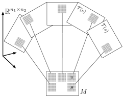
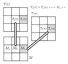
Figure 1: For illustrative purposes, we assume a distance function $d$ whose neighborhood structure coincides with the natural order on indices. That is, $s=(a,b)$ is similar to $u=(a^{\prime},b^{\prime})$ if $|a-a^{\prime}|$ and $|b-b^{\prime}|$ are small. (Left) For all $s\in[n_{1}]\times[n_{2}]$, the neighborhood $\{s^{\prime}:d(s,s^{\prime})<h\}$ in the original matrix $M$ is approximately described by the corresponding entries of the low-rank matrix $\mathcal{T}(s)$ (shaded regions of $M$ are matched by lines to the corresponding regions in $\mathcal{T}(s)$ that approximate them). If $d(s,u)$ is small, $\mathcal{T}(s)$ is similar to $\mathcal{T}(u)$, as shown by their spatial closeness in the embedding space $\mathbb{R}^{n_{1}\times n_{2}}$. (Right) The original matrix $M$ (bottom) is described locally by the low-rank matrices $\mathcal{T}(t)$ (near $t$) and $\mathcal{T}(u)$ (near $u$). The lines connecting the three matrices identify identical entries: $M_{t}=\mathcal{T}_{t}(t)$ and $M_{u}=\mathcal{T}_{u}(u)$. The equation at the top right shows a relation tying the three patterned entries. Assuming the distance $d(t,u)$ is small, $\epsilon=\mathcal{T}_{u}(t)-\mathcal{T}_{u}(u)=\mathcal{T}_{u}(t)-M_{u}(u)$ is small as well.

Without additional assumptions, it is impossible to estimate the mapping $\mathcal{T}$ from a set of $m<n_{1}n_{2}$ observations. Our additional assumption is that the mapping $\mathcal{T}$ is slowly varying. Since the domain of $\mathcal{T}$ is discrete, we assume that $\mathcal{T}$ is Hölder continuous. Following common approaches in non-parametric statistics, we define a smoothing kernel $K_{h}(s_{1},s_{2})$, where $s_{1},s_{2}\in[n_{1}]\times[n_{2}]$, as a non-negative symmetric unimodal function that is parameterized by a bandwidth parameter $h>0$. A large value of $h$ implies that $K_{h}(s,\cdot)$ has a wide spread, while a small $h$ corresponds to narrow spread of $K_{h}(s,\cdot)$. We use, for example, the Epanechnikov kernel, defined as $K_{h}(s_{1},s_{2})=\frac{3}{4}(1-d(s_{1},s_{2})^{2})\textbf{1}_{\{d(s_{1},s_{2})<h\}}$. We denote by $K^{(a,b)}_{h}$ the matrix whose $(i,j)$-entry is $K_{h}((a,b),(i,j))$.

Incomplete SVD (1) and compressed sensing (2) can be extended to local version as follows

Incomplete SVD: $$\ \ \hat{\mathcal{T}}(a,b)=\operatornamewithlimits{arg\,min}_{X}\|K^{(a,b)}_{h}\odot{\Pi}_{\mathtt{A}}(X-M)\|_{F}\ \ \;\text{s.t.}\quad\text{rank}(X)=r$$ (3)

Compressed Sensing: $$\ \ \hat{\mathcal{T}}(a,b)=\operatornamewithlimits{arg\,min}_{X}\|X\|_{*}\ \ \;\text{s.t.}\quad\|K^{(a,b)}_{h}\odot{\Pi}_{\mathtt{A}}(X-M)\|_{F}<\alpha,$$ (4)

where $\odot$ denotes a component-wise product of two matrices, $[A\odot B]_{i,j}=A_{i,j}B_{i,j}$.

The two optimization problems above describe how to estimate $\hat{\mathcal{T}}(a,b)$ for a particular choice of $(a,b)\in[n_{1}]\times[n_{2}]$. Conceptually, this technique can be applied for each test entry $(a,b)$, resulting in the matrix approximation $\hat{M}_{a,b}=\hat{\mathcal{T}}_{a,b}(a,b)$, where $(a,b)\in[n_{1}]\times[n_{2}]$. However, this requires solving a non-linear optimization problem for each test index $(a,b)$ and is thus computationally prohibitive. Instead, we use Nadaraya-Watson local regression with a set of $q$ local estimates $\hat{\mathcal{T}}(s_{1}),\ldots,\hat{\mathcal{T}}(s_{q})$, in order to obtain a computationally efficient estimate $\hat{\vphantom{\rule{1.0pt}{6.14584pt}}\smash{\hat{\mathcal{T}}}}(s)$ for all $s\in[n_{1}]\times[n_{2}]$:

$$\hat{\vphantom{\rule{1.0pt}{6.14584pt}}\smash{\hat{\mathcal{T}}}}(s)=\sum_{i=1}^{q}\frac{K_{h}(s_{i},s)}{\sum_{j=1}^{q}K_{h}(s_{j},s)}\,\hat{\mathcal{T}}(s_{i})~{}.$$ (5)

Equation (5) is simply a weighted average of $\hat{\mathcal{T}}(s_{1}),\ldots,\hat{\mathcal{T}}(s_{q})$, where the weights ensure that values of $\hat{\mathcal{T}}$ at indices close to $s$ contribute more than indices further away from $s$.

Note that the local version can be faster than global SVD since (a) each low-rank approximation is independent of each other, so can be computed in parallel, and (b) the rank used in the local SVD model can be significantly lower than the rank used in a global one. If the kernel $K_{h}$ has limited support ($K_{h}(s,s^{\prime})$ is often zero), the regularized SVD problems would be sparser than the global SVD problem, resulting in additional speedup.

3 Experiments

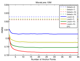
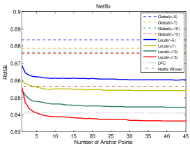
Figure 2: RMSE of global-LRMA, local-LRMA, and other baselines on MovieLens 10M (Left) and Netflix (Right) dataset. Local-LRMA models are indicated by thick solid lines, while global-LRMA models are indicated by dotted lines. Models with same rank are colored identically.

We compare local-LRMA to global-LRMA and other state-of-the-art techniques on popular recommendation systems datasets: MovieLens 10M and Netflix. We split the data into 9:1 ratio of train and test set. A default prediction value of 3.0 was used whenever we encounter a test user or item without training observations. We use the Epanechnikov kernel with $h_{1}=h_{2}=0.8$, assuming a product form $K_{h}((a,b),(c,d))=K_{h_{1}}^{\prime}(a,c)K_{h_{2}}^{\prime\prime}(b,d)$. For distance function $d$, we use arccos distance, defined as $d(x,y)=\arccos\left(\langle x,y\rangle/\|x\|\|y\|\right)$. Anchor points were chosen randomly among observed training entries. $L_{2}$ regularization is used for local low-rank approximation.

Figure 2 graphs the RMSE of Local-LRMA and global-LRMA as well as the recently proposed method called DFC (Divide-and-Conquer Matrix Factorization) as a function of the number of anchor points. Both local-LRMA and global-LRMA improve as $r$ increases, but local-LRMA with rank $r\geq 5$ outperforms global-LRMA with any rank. Moreover, local-LRMA outperforms global-LRMA in average with even a few anchor points (though the performance of local-LRMA improves further as the number of anchor points $q$ increases).