Magnetically Controlled Accretion on the Classical T Tauri Stars GQ Lupi and TW Hydrae

Abstract

We present high spectral resolution ($R\approx 108,000$) Stokes $V$ polarimetry of the Classical T Tauri stars (CTTSs) GQ Lup and TW Hya obtained with the polarimetric upgrade to the HARPS spectrometer on the ESO 3.6 m telescope. We present data on both photospheric lines and emission lines, concentrating our discussion on the polarization properties of the He I emission lines at 5876 Å and 6678 Å. The He I lines in these CTTSs contain both narrow emission cores, believed to come from near the accretion shock region on these stars, and broad emission components which may come from either a wind or the large scale magnetospheric accretion flow. We detect strong polarization in the narrow component of the two He I emission lines in both stars. We observe a maximum implied field strength of $6.05\pm 0.24$ kG in the 5876 Å line of GQ Lup, making it the star with the highest field strength measured in this line for a CTTS. We find field strengths in the two He I lines that are consistent with each other, in contrast to what has been reported in the literature on at least one star. We do not detect any polarization in the broad component of the He I lines on these stars, strengthening the conclusion that they form over a substantially different volume relative the formation region of the narrow component of the He I lines.

1. Introduction

T Tauri stars (TTSs) are young ($\lower 2.15277pt\hbox{$\;\buildrel<\over{\sim}\;$}10$ Myr), low mass ($\lower 2.15277pt\hbox{$\;\buildrel<\over{\sim}\;$}2.5$ M_⊙) stars that have only recently emerged from their natal molecular cloud cores to become optically visible. These young, low mass stars are generally subdivided into categories such as classical and weak TTSs. The designation of a classical TTS (CTTS) was originally based on a purely observational distinction: the equivalent width of the H$\alpha$ emission line. Classical TTSs are TTSs which have an H$\alpha$ equivalent width $W_{eq}(H\alpha)>10$ Å as distinguished from the weak line TTSs (WTTSs) defined by Herbig and Bell (1988); however, Bertout (1989) suggests that a break point value of 5 Å is more appropriate. More recently, investigators have tied the definition to the shape (width) of the H$\alpha$ line profile (e.g. White & Basri 2003, Jayawardhana et al. 2003). Independent of the exact constraint imposed for defining a CTTS, this moniker has become synonymous with a low mass pre-main star that is actively accreting material from a circumstellar disk. Indeed, the vast majority of stars which fit the criteria for CTTSs show some kind of additional evidence [e.g. inverse P-Cygni line profile shapes, optical veiling (see below), infrared excess] indicative of disk accretion.

It is now generally accepted that accretion of circumstellar disk material onto the surface of a CTTS is controlled by a strong stellar magnetic field (e.g. see review by Bouvier et al. 2007). These magnetospheric accretion models assert that strong stellar magnetic fields truncate the inner disk, typically near the corotation radius, and channel the accreting disk material onto the stellar surface, most often at high stellar latitude (Camenzind 1990; Königl 1991; Collier Cameron & Campbell 1993; Shu et al. 1994; Paatz & Camenzind 1996; Long, Romanova, & Lovelace 2005). More recent magnetohydrodynamic simulations find that outflows launched from near the region in which the stellar field interacts with the surrounding accretion disk can also spin the star down to observed rotation rates (e.g. Ferreira 2008; Romanova et al. 2009), though some recent work challenges the notion that these outflows can actually balance the spin-up accretion torques in CTTS systems (e.g. Zanni & Ferreira 2009).

Despite the successes of the magnetospheric accretion model, open issues remain. Most current theoretical models assume the stellar field is a magnetic dipole with the magnetic axis aligned with the rotation axis. However, recent spectropolarimetric measurements show that the fields on TTSs are probably not dipolar (Johns–Krull et al. 1999a; Valenti & Johns–Krull 2004; Daou, Johns–Krull, & Valenti 2006; Yang, Johns–Krull, & Valenti 2007; Donati et al. 2007, 2008, 2010a, Hussain et al. 2009). Few studies of accretion onto CTTSs have taken into account non-dipole field geometries. The earliest of these by Johns–Krull and Gafford (2002) found that abandoning the dipole assumption reconciled observed trends in the data with model predictions; however, this study did not consider the torque balance on the star and whether an equilibrium rotation rate could actually be achieved. Johns–Krull and Gafford (2002) argued that while the field on the stellar surface may be quite complex, the dipole component of the field should dominate at distance from the star where the interaction with the disk is taking place. This assumption appears to generally hold true in several recent studies (e.g. Johns–Krull & Gafford 2002; Mohanty & Shu 2008; Gregory et al. 2008; Long et al. 2008; Romanova et al. 2011; Cauley et al. 2012). However, the complex nature of the field near the surface has significant implications for the size of accretion hot spots, making them smaller than would be predicted by pure dipole models (Mohanty & Shu 2008; Gregory et al. 2008; Long et al. 2008); and also has important consequences for disk truncation radii and the computation of the torque balance on the star by the disk (Gregory et al. 2008; Long et al. 2008; Romanova et al. 2011).

Two approaches are generally used to measure magnetic fields on low mass stars, both utilizing the Zeeman effect. Magnetic fields can be measured from the broadening of magnetically sensitive lines observed in intensity spectra (e.g. Johns–Krull 2007; Yang et al. 2008). This technique is primarily sensitive to the magnetic field modulus, the unsigned value of the field weighted by the intensity distribution of the light emitted over the visible surface of the star. While this method does not suffer from flux cancellation due to regions of opposite polarity appearing on the star, it does require that all non-magnetic broadening mechanisms be accurately accounted for in the observed spectra. As a result, this technique is primarily sensitive to relatively strong fields. Observations of circular polarization in Stokes $V$ spectra can be much more sensitive to weak fields on the surface of stars; however, the Stokes $V$ signature is sensitive only to the line of sight component of the magnetic field and the signal can be reduced significantly due to flux cancellation when opposite field polarities are observed simultaneously on the stellar surface. Doppler shifts due to stellar rotation can reduce the degree of flux cancellation that results, permitting Stokes $V$ signatures to be present even when the net flux weighted line of sight field integrated over the stellar surface (the net longitudinal magnetic field, $B_{z}$) is zero. Observations of time series of Stokes $V$ spectra can be used to track changes in the amount of net field visible on the star as it rotates, ultimately allowing the large scale field of the star to be mapped using various tomographic imaging techniques (e.g. Donati et al. 2007 and references therein; Kochukhov et al. 2004 and references therein).

In addition to potentially mapping the surface field on accreting young stars, information can be obtained on the large scale field controlling the interaction of the star with its disk and the accretion flow by measuring time series of Stokes $V$ profiles in emission lines formed in the accretion flow and shock. The first accretion line for which circular polarization was detected is the He I line at 5876 Å (Johns–Krull et al. 1999a), and time series of the polarization variations in this line have been used to estimate the latitude of accretion spots on several CTTSs (e.g. Valenti & Johns–Krull 2004; Yang et al. 2007; Donati et al. 2008, 2010b, 2011a, 2011b). This line is observed in most CTTSs and is often found to be composed of two components: a narrow core component and a broad component extending out to several hundred km s^-1 (e.g. Edwards et al. 1994; Batalha et al. 1996; Alencar & Basri 2000). Based on the similarity in shape between the observed line profiles of some CTTSs and model profiles calculated in the context of magnetospheric accretion, Hartmann et al. (1994) suggested that the He I 5876 Å line (broad and narrow components) might form throughout the accretion flow, with the narrow component primarily coming from the lower velocity regions near the disk truncation point. Beristain et al. (2001) instead argue that the narrow core of the He I line arises in decelerating post-shock gas on the stellar surface at the base of the accretion footpoints. Beristain et al. (2001) argue that the broad component observed in many CTTSs has a dual origin in the magnetospheric flow and in a high velocity wind in the most strongly accreting stars.

The strong, ordered fields observed in the narrow component of this line component ($\sim 2.5$ kG, e.g. Johns–Krull et al. 1999a) argue for a formation region close to the stellar surface instead of several stellar radii above the star where the field interacts with the disk. The He I 5876 Å arises from a triplet state and is composed of several closely spaced lines. The He I 6678 Å line arises from the analogous singlet state, and is observed in many CTTSs as well where it displays both broad and narrow components (see Beristain et al. 2001). Based on the strong similarity in their kinematic properties and the measured triplet-singlet flux ratio, Beristain et al. (2001) conclude that the narrow component of both He I lines forms in the post-shock gas. On the other hand, this picture is complicated by the observation of Donati et al. (2008) that the 6678 Å line consistently shows a longitudinal magnetic field strength approximately twice that of the 5876 Å line in the CTTS BP Tau whose He I lines are dominated by a narrow component (Edwards et al. 1994, Batalha et al. 1996, Beristain et al. 2001). This is a surprising observation since models of accretion shocks on CTTSs find that the thickness of the post-shock region is typically $10^{5}-10^{6}$ cm (Calvet & Gullbring 1998; Lamzin 1998) which is a small fraction ($\lower 2.15277pt\hbox{$\;\buildrel<\over{\sim}\;$}10^{-5}$) of a stellar radius. It would be surprising if the stellar magnetic field strength varied so strongly with depth, suggesting then that perhaps the two He I lines do not trace the same regions on the stellar surface.

To better clarify the magnetic field properties of accretion related lines, more spectropolarimetric observations of CTTSs, including those with substantial broad components to their He I lines, are needed. Here, we report new observations of two CTTSs (GQ Lup and TW Hya) using the newly commissioned polarimeter operating with the HARPS spectrograph on the ESO 3.6 m telescope at La Silla. TW Hya is a K7 CTTS and a member of the loose TW Hydrae association (Kastner et al. 1997). The Hipparcos parallax for TW Hya implies a distance of $56\pm 7$ pc (Wichmann et al. 1998), making it the closest CTTS to the Earth. Based on its placement in the HR diagram, the age of TW Hya is estimated to be 10 Myr (Webb et al. 1999, Donati et al. 2011b). Setiawan et al. (2008) claimed the detection of a $\sim 10$ M_Jup planet in a very close orbit around this CTTS, making TW Hya an important benchmark constraining the timescale of planet formation. Huélamo et al. (2008) instead suggest that the observed radial velocity variations which signal the presence of the planet are in fact caused by large starspots on the surface of TW Hya. As a result, there is great interest in knowing as much about this star as possible. In addition, TW Hya is still accreting material from its circumstellar disk and is observed at a low inclination ($i\sim 18^{\circ}$, Alencar & Batalha 2002), making it an excellent object for studying magnetically controlled accretion onto young stars. The magnetic properties of TW Hya have been investigated a number of times previously (Yang et al. 2005, 2007; Donati et al. 2011b). GQ Lup is also a K7 CTTS, and has also recently come under a great deal of scrutiny as the result of a claimed planetary mass companion. Neuhäuser et al. (2005) discovered an infrared companion at a separation of $\sim 0.^{\prime\prime}7$ (corresponding to $\sim 100$ AU at a distance of 150 pc). Based on their infrared photometry and K band spectra, Neuhäuser et al. (2005) constrained the mass of GQ Lup B to be between $1-42$ M_Jup, placing it possibly in the planet regime. More recent spectroscopic studies have favored the upper end of this range, suggesting the companion is more likely a brown dwarf (Mugrauer & Neuhäuser 2005; Guenther et al. 2005; McElwain et al. 2007; Seifahrt et al. 2007; Marois et al. 2007; Neuhäuser et al. 2008). The formation of such an object presents challenges to theories of companion formation in a disk, and has sparked continued study of this system to better pin down the properties of both of its members. GQ Lup is known to show clear signs of variable accretion (Batalha et al. 2001), making it a good target to study the role of magnetic fields in the accretion process. To our knowledge, no studies of the magnetic properties of GQ Lup exist to date. In §2 we describe our observations and data reduction. The magnetic field analysis and results are described in §3, and in §4 we discuss the implications of our findings.

2. Observations and Data Reduction

All spectra reported here were obtained at the ESO 3.6 m telescope on La Silla using the newly comissioned polarimeter, HARPSpol (Snik et al. 2008, 2011; Piskunov et al. 2011), mounted in front of the fibers feeding the HARPS spectrometer (Mayor et al. 2003). While HARPSpol can also record Stokes $Q$ and $U$ spectra, for the observations reported here, only Stokes $V$ spectra were obtained. As mentioned above, linear polarization in both the lines and the continuum can result from scattering off a circumstellar disk (e.g. Vink et al. 2005); however, the action of a disk does not typically produce circular polarization in either the lines or the continuum. Here, we will focus only on Stokes $V$ in the lines measured relative the continuum which is assumed to not be circularly polarized. With this instrumental setup, each exposure simultaneously records the right and left circularly polarized components of the $R=108,000$ spectrum. These two components of the echelle spectrum are interleaved, such that two copies of each echelle order are present on the two $2148\times 4096$ CCD arrays (one for the blue portion of the spectrum and one for the red). The two polarized components of each order are separated by $\sim 16$ pixels in the cross dispersion direction on the array, while each spectral trace is $\sim 3.5$ pixels wide (FWHM) in the cross dispersion direction. Each observation of a star reported here actually consists of 4 separate observations of the star, with the angle of the quarter waveplate in the polarimeter advanced by 90^∘ between the exposures. The result of this is to interchange the sense of circular polarization in the two beams. This gives substantial redundancy in the analysis which allows us to remove most potential sources of spurious polarization due to uncalibrated transmission and gain differences in the two beams. As described below, we use the “ratio” method to combine the spectra from these interchanged beams in order to form Stokes $I$ and $V$ spectra that are largely free of these potential spurious signals (e.g. Donati et al. 1997; Bagnulo et al. 2009). All spectra were obtained on the nights 29 April 2010 through 2 May 2010, with one night (1 May) lost due to weather. Table 1 gives a complete table of the stellar observations reported here. Included in the Table are continuum signal-to-noise estimates near the two He I emission lines studied here as well as the emission equivalent widths of these two lines. Also reported is the veiling found near the He I 6678 Å line as discussed below. Along with spectra of GQ Lup and TW Hya, a spectrum of the weakly accreting TTS V2129 Oph was also obtained and is used in the analysis of the He I lines on the other stars. In addition to stellar spectra, standard calibration observations were obtained including bias frames, spectra of a Thorium Argon lamp for wavelength calibration, and spectra of an incandescent lamp for the purpose of flat fielding. The calibration spectra were obtained with the polarimeter in front of the fibers.

All spectra were reduced with the REDUCE package of IDL echelle reduction routines (Piskunov & Valenti 2002) which builds on the data reduction procedures described by Valenti (1994) and Hinkle et al. (2000). The reduction procedure is quite standard and includes bias subtraction, flat fielding by a normalized flat spectrum, scattered light subtraction, and optimal extraction of the spectrum. The blaze function of the echelle spectrometer is removed to first order by dividing the observed stellar spectra by an extracted spectrum of the flat lamp. Final continuum normalization was accomplished by fitting a 2nd order polynomial to the blaze corrected spectra in the regions around the lines of interest for this study. Special care was taken to apply a consistent continuum normalization procedure to the spectra extracted from all four sub-exposures. Occasional small difference in normalization of the two orthogonal spectra are compensated by using the “ratio” method (e.g. Bagnulo et al. 2009, and below) to combine the right and left circularly polarized components. The wavelength solution for each polarization component was determined by fitting a two-dimensional polynomial to $n\lambda$ as function of pixel and order number, $n$, for approximately 1000 extracted thorium lines observed from the internal lamp assembly. The resolution as determined by the median FWHM of these thorium lines was $R=107,660$.

As mentioned above, each subexposure obtained of a given star contains both the right and left circularly polarized component of the spectrum. In order to get a final measurement of the mean longitudinal magnetic field, $B_{z}$, these individual measurements of the two circular polarization components must be combined in some way. We used the “ratio” method (e.g. Bagnulo et al. 2009, Donati et al. 1997) to combined the right and left circularly polarized components of the spectra form the Stokes $V$ spectrum as well as a null spectrum, with each being renormalized to the continuum intensity. We also added all the components together to form the Stokes $I$ spectrum. With Stokes $V$ and $I$ determined, the continuum normalized right-hand circularly polarized (RCP) component of the spectrum is then $R=I+V$ and the continuum normalized left-hand circularly polarized (LCP) component of the spectrum is $L=I-V$. Computing these from $I$ and $V$ in this way ensures both circular polarization states have been normalized to the same continuum.

3. Analysis

3.1. He I Line Equivalent Widths

Table 1 gives the equivalent width of the two He I lines studied here for all our target stars. As mentioned before, previous investigators have noted that these lines often appear to have two distinct components (e.g. Batalha et al. 1996; Beristain et al. 2001): a narrow component (NC) and broad component (BC). It is thought that the two components may form in different physical regions of the accretion flow onto CTTSs (Beristain et al. 2001) and their polarization properties also appear to be different with the narrow compnent showing significantly stronger polarization (Daou et al. 2006; Donati et al. 2011b). We therefore report the equivalent width of the NC and the BC separately for the two He I lines, the sum giving the total line equivalent width. Decomposing the lines in this manner requires some assumptions to be made about how to separate the two components. Since the NC often appears asymmetric (e.g. Figure 1) with a very steep blue edge and shallower red edge, Gaussian fitting to the lines requires particular choices to be made on just how to do the analysis. For example, Batalha et al. (1996) define (by eye) a region outside the NC and fit a single Gaussian to the resulting BC and subtract it off in order to measure the NC equivalent width. Another procedure is to fit the entire line with multiple Gaussians and use the resulting fit parameters to estimate component properties (e.g. Alencar & Basri 2000). The resulting equivalent with of the various features then depedns at some level on how one chooses to do the analysis. This is illustrated in Figure 1. The top panel shows the He I 5876 Å line of TW Hya from the first night. The smooth solid curve shows a line profile fit employing 3 Gaussian components. The dash-dot line shows a fit using only two Gaussian components. There is a clear difference in the two fits (the 3 Gaussian fit uses two Gaussians to fit the NC which is not really Gaussian as mentioned above).

The bottom panel of Figure 1 zooms in on the line to show the recovered BC profiles. The BC from the 3 Gaussian fit is shown in the smooth solid line and that from the two Gaussian fit is shown in the dash-dot line. Also shown is a BC fit (dash-triple dot line) following Batalha et al. (1996) where a single Gaussian is used to fit the region outside the NC. Finally, the solid straight line connecting the two large squares shows a by eye estimate of the point on both the blue and red side of the line (as seen in Stokes $I$) where the NC and BC join with a linear interpolation between these points to define the separation of the NC and the BC which can be used to separately determine their equivalent widths. This then gives 4 different ways to estimate the equivalent width of the BC (and also the NC). The two extremes for the BC equivalent width are the single Gaussian fit (1.193 Å) following Batalha et al. and that (1.089 Å) from the two Gaussian fit, corresponding to a difference of 9%. Clearly, none of the Gaussian fits exactly follow the red side of the BC, so it is impossible to predict just what this component does under the NC. Given this uncertainty and the fact that using the linear interpolation between the blue and red sides of the apparent boundary between the NC and BC gives equivalent width values between the two extremes, we choose to use this method to separate both components and measuure the equivalent widths reported in Table 1. We note that the BC equivalent width for the profile shown in Figure 1 computed this way differs from that resulting from the 3 Gaussian fit by only 4.9%. We therefore estimate that the systematic uncetainty resulting from the choice of just how to separate the two components likely leads to a 5% uncertainty in the reported equivalent widths which is not included in the Table. In most cases, the boundary between the BC and the NC is clear and repeated measurements with slightly different choices yield results with a difference less than $1\sigma$ for the quoted uncertainties. There are a few cases where the boundary between the NC and the BC, or the BC and the continuum, are less clear and we repeated the measurements with a larger distinction in our choices of these points. These are noted Table 1 and we use our different measurement trials to estimate the the equivalent width uncertainty for these profiles. For the other measurements, the uncertainties are computed by propagating the uncertainties in the observed spectra.

3.2. The Photospheric Mean Longitudinal Field

For each of the T Tauri stars, we measured the photospheric $B_{z}$ using approximately 40 magnetically sensitive absorption lines (Table 2), which form primarily over the portions of the stellar surface that are at photospheric temperatures. These lines may have relatively little contribution from the cool spots that are likely present on these stars. Due to the wavelength dependence of the Zeeman effect and the fact that the signal-to-noise ratio achieved in the observations of these late-type stars is considerably higher in the red regions of spectrum, we focus the analysis here only on the spectra from the red CCD of HARPSpol. Lines for the analysis were selected by visual inspection of all the orders on the red CCD recorded with HARPS. Lines were deemed good for the analysis if they appeared relatively strong (central depth $\lower 2.15277pt\hbox{$\;\buildrel>\over{\sim}\;$}0.15$) in the observed spectrum (though most were considerably stronger), appeared free of blending by other photospheric lines, and were not contaminated by telluric absorption. Lines passing these criteria were then checked in the Vienna Atomic Line Database (VALD, Kupka et al. 1999, 2000) and if they are present and have a value for the effective Landé $g$-factor, the line was used in the analysis. In a few cases, the VALD data indicated that an apparently good line is actually a very close blend of two lines. In this case, we used the line but estimated a new effective Landé $g$-factor by calculating the weighted mean of the effective Landé $g$-factors of the lines in the blend. The weights used are the central depth of each component line as predicted by VALD for the atmospheric parameters typical of K7 TTS ($T_{eff}=4000$ K, log$g=3.5$). The initial line list was constructed using a visual examination of the spectrum of GQ Lup obtained on 29 April 2010. For the other TTSs some lines were affected by blending with telluric absorption or by strong cosmic ray hits (as is also the case for later observations of GQ Lup). In these cases, the lines were not included in the determination of the photospheric $B_{z}$ values. Lines so affected are noted in Table 2.

Once the line list was determined, the mean longitudinal magnetic field, $B_{z}$, can be estimated by measuring the wavelength shift of each line, $\Delta\lambda=\lambda_{R}-\lambda_{L}$, where $\lambda_{R}$ is the wavelength of the line observed in the RCP component of the spectrum and $\lambda_{L}$ is the wavelength measured in the LCP component of the spectrum (Babcock 1962). The shift of the line observed in the two polarization states is related to $B_{z}$ by

$$\Delta\lambda=2{e\over 4\pi m_{e}c^{2}}\lambda^{2}g_{\rm{eff}}B_{z}=9.34\times 10^{-7}\lambda^{2}g_{\rm{eff}}B_{z}\,\,\,\,\,\,\rm m\mbox{\AA}\,$$

where $g_{\rm{eff}}$ is the effective Landé $g$-factor of the transition, $B_{z}$ is the strength of the mean longitudinal magnetic field in kilogauss, and $\lambda$ is the wavelength of the transition in Angstroms (Babcock 1962; see also Mathys 1989, 1991). In order to measure the wavelength shift, $\Delta\lambda$, we measured the wavelength of each line of interest in the two circular polarization components using the so-called center of gravity method (e.g. Mathys 1989, 1991; Plachinda & Tarasova 1999). This method for estimating $B_{z}$ is mathematically equivalent to estimating $B_{z}$ from the first order moment of the Stokes $V$ profile, assuming the same integration limits are used in the two methods (e.g. Borra & Vaughn 1977; Mathys 1989; Landi Degl Innocenti 2004). Determining $B_{z}$ requires knowledge of the effective Landé $g$-factor, $g_{\rm eff}$, for the transition. The weights for individual $\pi$ and $\sigma$ components of a given spectral line which go into the definition of $g_{\rm eff}$ assume an optically thin line, so equation (1) is only approximately true in the case of moderately strong (saturated) photospheric lines. As a result, using equation (1) is strictly valid only for weak lines, but give good results for real spectral lines (Mathys 1991). For each measurement of the center of gravity of a spectral line, we used the locally measured signal-to-noise in the spectrum to estimate the uncertainty in the spectrum and then used standard error propagation to find the uncertainty in the line shift bewteen the two polarization states and the implied $B_{z}$. Our final estimate of $B_{z}$ is a weighted mean of the individual line estimates, and these means are reported in Table 3.

We repeated the measurements of the line wavelengths in the two polarization components and the resulting final value of $B_{z}$ a number of times, making slightly different choices on integration limits for the center of gravity estimate of the wavelength of each line. However, for each trial we always used the same integration limits for a given line when analyzing the RCP and LCP components of the spectra. In each case, we achieved consistent results within our quoted uncertainties. Generally, we divided our trials in two groups. In the first case, we choose integration limits very close to where the lines appear to reach the local continuum. This was primarily done as an effort to exclude any potential weak line blends that might appear as a small distortion in the line wings. In the second group, we choose integration limits clearly out in the local continuum, but which in some cases likely included some weak line blends. In many cases, choosing the wider limits produced higher values of $B_{z}$, though in some cases the measured field went down. On average, the wider bins resulted in fields stronger by $\sim 35$%. Choosing the wider limits does generally result in somewhat larger uncertainty estimates, typically by a factor of 1.8. Again, the two groups of results are consistent within these uncertainties (the difference typically being $\sim 1.5\sigma$). In Table 3 we quote the values for the wider integration limits with their correspondingly greater uncertainties.

Examining the photospheric fields and their uncertainties as reported in Table 3, apparently significant fields are found on both TW Hya and GQ Lup each night they were observed. However, the value of $B_{z}$ found on V2129 Oph is less than $1\sigma$ and does not represent a real detection. As a test of our measurement techniques and in order to gain confidence in our uncertainty estimates, two different null tests were performed on the observations of each target. Each test should return a measured value of $B_{z}=0$, thus serving to test how accurately we can recover this value and whether the uncertainties are realistically estimated. As described above, the spectra from the 4 subexposures were also combined in such a way as to produce a null Stokes $V$ profile (e.g. Donati et al. 1997; Bagnulo et al. 2009), which can be used to calculate null RCP and LCP spectra. We analyzed these null spectra in the same as described above. This has the advantage of using exactly the same lines as used to measure $B_{z}$, with exactly the same wavelength limits for computing the shift of each line, but with data combined in a different way than in the real measurement. The second null test we employed used 15 strong telluric lines from the atmospheric B band of oxygen between 6883 - 6910 Å. Since these lines should show no significant polarization of their own, we can analyze them in exactly the same fashion as we do the stellar lines from which we derive $B_{z}$ (that is we take $\Delta\lambda=\lambda_{R}-\lambda_{L}$ as done for the stellar measurements) combining the data from the sub-exposures in exactly the same way as done for the stellar measurements. In order to translate the measured shifts to a value of $B_{z}$ we assign a Landé $g$-factor to each telluric line equal to the mean value of the photospheric lines used for the given observation. The weights are the uncertainty on the value of $B_{z}$ derived from each of the photospheric lines. These null test field values are also reported in Table 3.

3.3. $B_{z}$ in the Accretion Shock Emission

As described above, Johns–Krull et al. (1999a) discovered that the He I 5876 Å emission line can be circularly polarized in spectra of CTTS, implying coherent magnetic fields at the footpoints of accretion columns. They measured $B_{z}=2.46\pm 0.12$ kG for BP Tau. Since this original discovery, polarization in the He I 5876 Å emission line has now been reported for a number of CTTSs by a number of investigators (Valenti & Johns–Krull 2004; Symington et al. 2005; Smirnov et al. 2004; Yang et al. 2007; Donati et al. 2007, 2008, 2010b; Chen & Johns–Krull 2011). Polarization has since been detected in other emission lines (notably He I 6678 Å and the Ca II IRT lines) thought to be associated with accretion shock emission as well (Yang et al. 2007; Donati et al. 2007, 2008, 2010b; Chen & Johns–Krull 2011). The spectra obtained here contain both the He I 5876 Å and 6678 Å lines, so we analyze them with a focus on trying to see how well the fields derived from each line agree with one another as this could provide clues to the location and geometry of the accretion shocks on the star. As mentioned earlier, the 5876 Å line of He I is composed of several components (6) which are closely spaced in wavelength, and as a result is subject to the Paschen-Back effect (e.g. Yang et al. 2007; Asensio Ramos et al. 2008). Therefore, the exact splitting pattern of the lines can vary considerably, depending on the strength of the magnetic field. However, since most of the level crossing and merging has occurred by the time the local field strength reaches 2 kG (e.g. Asensio Ramos et al. 2008), the He I 5876 Å line should be in or very close to the complete Paschen-Back limit given the field strengths we recover below. As a result, we set $g_{eff}=1.0$ for this line as done in Yang et al. (2007). We can then test the validity of this assumption once we have our field measurements.

Figure 2 shows the right- and left-circularly polarized components of the He I 5876 Å emission lines of GQ Lup and TW Hya as observed on 29 April 2010. Also shown in the figure are the Stokes $V$ profiles of the lines. Nearby photospheric absorption lines are also seen in each star. Since the polarization signal in the photosphere is quite weak due to the low value of $B_{z}$ present there (Table 3), these individual photospheric absorption lines do not show obvious polarization. They do serve to show that the two polarization components are well aligned in wavelength, so that the obvious shift of the He I emission line between the RCP and LCP components indicates a very strong field in the line formation region.

In order to measure the value of $B_{z}$ in the line formation region of the He I line we again use the center of gravity technique to measure the wavelength shift of the line as observed in the two polarization components (RCP and LCP). Our measurements of $B_{z}$ and its uncertainty for both He I emission lines are reported in Table 3 for each star on each night. When measuring the field in the He I formation region, care must be given when selecting the wavelength limits for determing the center of gravity wavelength of the line and also in deciding how to separate the narrow (NC) and broad (BC) components of the line (§3.1). Looking at the He I 5876 Å line of TW Hya in Figures 1 and 2, polarization is clearly seen in the NC of the line, but is not obviously apparent in the BC extending off to the red side of the line. As a result, we focussed in on the NC of the line when measuring the value of $B_{z}$ in the 5876 Å line of He I.

In addition to the specific wavelength region chosen, care must also be taken when defining the local continuum to be used when measuring the center of gravity wavelength for the line. The reason for this is that the center of gravity technique (as well as the first moment of Stokes $V$) is an intensity weighted mean wavelength, where the intensity used is that above the continuum in the case of an emission line. In the case of the He I 5876 Å emission line, the NC of the line sits on top of a BC in many cases as discussed above. In this case, significantly different results are obtained if the stellar continuum is used compared to what is obtained if a somewhat higher continuum defined by the BC is used. We proceed in an effort to isolate the emission from the NC and measure $B_{z}$ in this component. Interpreting the NC of the He I emission as an excess line emitted from a distinct region that adds its emission to that from both the stellar continuum and the BC of the He I emission, these additional sources should be subtracted off when measuring the center of gravity wavelength of the NC of the emission line. In §3.1 we described several methods of separating the NC and BC when measuring their equivalent width, showing that each method is subject to certain biases, but that the resulting systematic differences were small ($\sim 5$% for the method we settle on). We used the same methods to remove the BC from the line (each BC is shown in the bottom of Figure 1) and measured the resulting $B_{z}$. For the profile shown in Figure 1, using the single Gaussian fitted to the region outside the NC gave the largest magnitude field ($-2.57\pm 0.11$ kG), while the two Gaussian fit and the linear interpolation both gave $-2.38\pm 0.10$ kG, and the 3 Gaussian fit gave $-2.40\pm 0.11$ kG. All 4 methods give results consistent to within 2$\sigma$ and three of the 4 differ by 0.02 kG or less. As in the case for the equivalent widths above, we again adopt the linear interpolation under the NC as the way of removing the BC and use the resulting NC to determine the $B_{z}$ values given in Table 3.

As mentioned earlier, there have been reports in the literature that the He I 6678 Å line shows substantially stronger polarization than the 5876 Å indicative of a stronger local field in the line formation region of this more optically thin line. We looked for evidence of this effect in our stars by analyzing the the 6678 Å emission line in all 3 of the T Tauri stars oberved here in a way similar to how the the 5876 Å line is analyzed. However, it became immediately apparent that additional care needs to be taken when analyzing the 6678 Å line. Figure 3 illustrates the situation for GQ Lup with the spectrum obtained on the first night of our observing run. Shown in the figure is the right and left circularly polarized components of the spectrum, along with the Stokes $V$ profile. Unlike the 5876 Å line where the right and left circularly polarized components of the emission line have essentially the same shape, only shifted, the 6678 Å line of GQ Lup has a different shape in the two circular polarization components. On the other hand, the Stokes $V$ profile for the two He I lines looks quite similar. The reason this is the case is the presence of an Fe I photospheric absorption line at the same wavelength of the 6678 Å line which can be seen in the spectrum of V2129 Oph (taken on night 2) which is also shown in Figure 4. In V2129 Oph, the He I 6678 Å line shows no obvious emission, but it turns out there is some weak emission in this line in V2129 Oph that partially fills in the photospheric absorption line and produces a clear Stokes $V$ signature which is illustrated in Figure 4 and discussed below.

As described above, the formation region for the narrow components of these He I lines is thought to be at the base of the accretion columns where material from the disk is raining down onto the star. In addition to producing some emission lines, these accretion footpoints are believed to be the source of the optical continuum veiling seen in most CTTSs (e.g. Basri & Batalha 1990; Hartigan et al. 1991; Valenti et al. 1993; Gullbring et al. 1998). This extra line and continuum emission region effectively blocks some small portion of the stellar surface and the light it emits, adding its own emission on top of the stellar spectrum coming from the non-accreting regions of the star (e.g. Cavet & Gullbring 1998). The spectrum of the excess can then be studied by subtracting an appropritely scaled (veiled) stellar template spectrum from the observed CTTS spectrum (e.g. Hartigan et al. 1995; Gullbring et al. 1998; Stempels & Piskunov 2003). The spectrum of the excess is sometimes studied by subtracting off the spectrum of a veiled WTTS or main sequence star of the same spectral type, while other studies use a synthetic spectrum computed from a model stellar atmosphere. Here, we use a model stellar atmosphere since we did not observe a suitable WTTS having no excess continuum or line emission of its own.

The top panel of Figure 3 shows a portion of the spectrum of V2129 Oph in the neighborhood of the He I 6678 Å line with our best fit synthetic spectrum including a modest amount of veiling ($r=0.17$, that is, a continuum excess equal to 0.17 of the local stellar continuum) added in. This value for the veiling is slightly higher than previously reported values for V2129 Oph: $r=0.0\pm 0.1$ (Basri & Batalha 1990); $r=0.075\pm 0.020$ (Donati et al. 2011a, though this is only a relative veiling value and represents a lower limit to the true value). For our purposes, the exact value of the veiling is not important. The primary goal with such a fit is to predict the strength of the Fe I absorption line at 6678 Å. To do so, we synthesize the spectral region between 6660 – 6680 Å as shown in Figure 4. The two strongest features in this region are the Fe I feature at 6678 Å and another Fe I feature at 6663 Å. Both of these features seen in Figure 4 are actualy blends of two Fe I lines. However, since all the components of both features are from the same element in the same ionization stage, it should be possible to “fit” the 6663 Å feature and then predict the strength of the 6678 Å line. We use the spectrum synthesis code SYNTHMAG (Piskunov 1999). The line data for this spectral region is taken from VALD (Krupka et al. 1999, 2000). As is often the case, the initial predicted line strengths do not match up well with observations of the TTSs or the Sun, so we tuned the oscillator strengths (and in a few cases the Van der Waals broadening constants) of the strong lines until a good match with the solar atlas (Kurucz et al. 1984) was obtained. In tuning the line parameters to the solar spectrum, we use the model atmosphere and associated parameters ($v$sin$i$, macroturbulence, etc.) for the $T_{eff}=5731$ K scaled Kurucz model from Valenti and Piskunov (1996). Once the line data is set, we then synthesize this same spectral region for each of our CTTSs using NextGen model atmospheres (Allard & Hauschildt 1995). To do so, we must select an effective temperature, gravity, and metallicity for each star. We take the gravity as log$g=3.5$ and metallicity as [M/H] = 0.0 for all stars; however, we pick effective temperatures from the standard NextGen grid that are as close as possible to that for each star. Donati et al. (2007) adopt an effective temperature of $4500\pm 200$ K for V2129 Oph, and we adopt the NextGen model with $T_{eff}=4600$ K for this star. Yang et al. (2005) find $T_{eff}=4126\pm 24$ K for TW Hya, and we adopt the NextGen model with $T_{eff}=4200$ K. GQ Lup has the same spectral type as TW Hya (K7), so we use the same NextGen model for this star as well. In order to do the final spectrum synthesis and fitting to the observed profile, we must select the micro and macroturbulence as well as the $v$sin$i$ rotational velocity. Following Johns–Krull et al. (1999b) we take 2.0 km s^-1 for the macroturbulent velocity and set the microturbulence to 1.0 km s^-1. In order to account for rotation, we set $v$sin$i=4.0$ km s^-1 for TW Hya (Donati et al. 2011b), we set $v$sin$i=14.5$ km s^-1 for V2129 Oph (Donati et al. 2007), and we set $v$sin$i=6.8$ km s^-1 for GQ Lup (Guenther et al. 2005).

Using the spectrum synthesis described above, we match the strength of the Fe I feature at 6663 Å and subtract the model spectrum from the right and left circularly polarized components of the observed spectrum, add a pseudo-continuum of 1.0 back in, and then follow the procedure described above for the He I 5876 Å line in order to measure the field in the formation region of the 6678 Å He I line. The only free parameter used to fit the 6663 Å Fe I is the value of the continuum veiling. These veiling values and the $B_{z}$ values for the 6678 Å emission line are reported in Table 1. In general our veiling values agree well with previously published determinations considering this quantity is often quite variable in CTTSs. In addition to previous veiling measurements for V2129 Oph discussed above, veiling on TW Hya in similar spectral regions has been shown to vary, reaching as high as 0.80 in the study of Alencar and Batalha (2002) and as high as $\sim 0.92$ in the work of Donati et al. (2011b). In the case of GQ Lup, Weise et al. (2010) found a veiling of 0.5 near the Li I line at 6707 Å, while here we find values ranging from 0.3 to 0.6. Again though, the exact value of the veiling is of secondary importance: accounting for the photospheric absorption which is coincident with the He I 6678 Å emission makes a substantial difference in the recovered field strengths for this line. To gauge this effect, we repeated the analysis of the 6678 Å line without making any correction for the photospheric absorption present. Generally, the fields we measure in this case are a factor of two larger than those reported in Table 3.

4. Discussion

Examining both the null Stokes $V$ field values and the field values obtained from the analysis of the telluric lines shows that each of these is quite low and generally equal to zero (as they should be) within the measured uncertainties. In the case of the null spectrum, the value reaches a significance of $3.3\sigma$ in one case, but most values are between $1-2\sigma$. For the telluric lines, all of the measured $B_{z}$ values are equal to zero (as expected) to within $1\sigma$ or less. The uncertainties from the telluric tests are also generally lower than the for the photospheric lines (both actual measurement and null test). This is primarily due to the telluric lines being very sharp and strong, allowing for very accurate measurements of any potential wavelength shift. We conclude from these tests that our uncertainties in $B_{z}$ are generally well characterized and that our detections of polarization in the photospheric lines and resulting measurements of $B_{z}$ on GQ Lup and TW Hya are real.

TW Hya has been studied with spectropolarimetry by Yang et al. (2007) and Donati et al. (2011b). On one of six nights, Yang et al. (2007) measured polarization in a dozen photospheric lines of TW Hya corresponding to a longitudinal magnetic field of $B_{z}=149\pm 33$ G, while finding no significant polarization (though with larger uncertainties) on the other five nights. Donati et al. (2011b) observed TW Hya for a total of 20 nights and used their least squares deconvolution (LSD) analysis (Donati et al. 1997) to measure photospheric fields ranging from $B_{z}=380-700$ G with uncertainties typically of 15 G. Donati et al. suggest that long term temporal variability may be responsible for the variations in $B_{z}$ between the measurements of Yang et al. (taken in April 1999) and those of Donati et al. (taken in March 2008 and March 2010). The results presented here, from April and May 2010, agree well with those of Yang et al. and less so with those of Donati et al. (2011b).

Yang et al. (2007) measured polarization in the He I 5876 Å and 6678 Å emission lines of TW Hya, as well as in the Ca II 8498 Å emission line. Yang et al. report possible rotational modulation of the polarization in the He I 5876 Å line, with implied fields varying from $\sim-1450$ to $\sim-1800$ G. Donati et al. (2011b) also measure strong polarization in the He I 5876 Å line with variations again suggestive of rotational modulation. The field strength implied in this case ranges from $\sim-2000$ to $\sim-3500$ G. Donati et al. attribute the significant difference between their He I measurements and those of Yang et al. to perceived differences in the way the fields were measured in the two studies. Donati et al. measured the field only in the narrow component of the line for similar reasons to those cited above in §3.3, and they state that Yang et al. (2007) used the entire He I line in their field determination; however, this is not correct. Yang et al. (2007) also focussed only on the narrow component of the He I emission line in their field determinations (Yang, private communication). The field measurements reported here in Table 3 for $B_{z}$ in the He I 5876 Å emission line generally agree well with those of Yang et al. and are significantly less than most of the fields reported by Donati et al. However, Yang et al. used a cross correlation technique to measure line shifts and resulting field strengths, while here we use the center of gravity technique to measure line shifts.

In order to verify that the difference in measurement technique does not introduce a spurious difference in the recovered field, we reanalyzed the Yang et al. (2007) spectrum of TW Hya obtained on 21 April 1999 (the strongest He I field they found) using the same center of gravity technique employed above. Briefly, this spectrum was obtained with the 2.7 m Harlan J. Smith telescope of McDonald Observatory used to feed the Robert G. Tull coude echelle spectrometer (Tull et al. 1995). The starlight was split into its circularly polarized components using a Zeeman Analyzer (ZA, Vogt et al. 1980) placed in front of the spectrometer slit. The ZA contains a Babinet-Soleil phase compensator used to correct for a potential reduction in sensitivity to circular polarization which can be introduced by the non-azimuthally symmetric reflections in the coude mirror train. Such bounces can introduce some linear polarization into an originally circularly polarized beam and the phase compensator is used to convert this linear polarization back into the original circular polarized signal (see Vogt et al. 1980 and Vogt 1978). The exposure of TW Hya for that night totalled 4300 s. Yang et al. (2007) measured a field of $-1806\pm 114$ G for the narrow component of the He I 5876 Å line using a cross correlation analysis, while we find a field of $-2326\pm 118$ G using the center of gravity technique, fully consistent with our current measurements. This measurement of the field is stronger by $520\pm 164$ G than that of Yang et al. (2007), representing a $3.2\sigma$ difference. The difference is driven both by the method of estimating the line shift (center of gravity versus cross correlation) as well as in the treatment of removing the broad component. As a result, it does not appear that differences in the measurement technique can account for the variations in the field strength in the He I emission line formation region found between Donati et al. (2011b) and this study plus that of Yang et al. (2007). It is more likely that intrinsic variability is at work in this accretion diagnostic, and indeed, Donati et al. (2011b) find significant differences in the He I field strength from one rotation phase to the next in TW Hya, while the bulk of their field measurements are larger in magnitude than either Yang et al. (2007) or those here.

One of the motivations for this study was to verify and expand on the intriguing result that the field measured from the He I 6678 Å line is significantly different (stronger) than that measured in the He I 5876 Å line (e.g. Donati et al. 2008). In principle, measuring the field in different emission line diagnostics could offer a means for probing the magnetic field structure through the accretion shock on CTTSs. As described in §3.3, we discovered that there is a strong photospheric Fe I absorption line coincident in wavelength with the He I 6678 Å line that can severely affect the field strength measured in this emission line if the photospheric line is not properly accounted for. As described above, we attempted to correct for the Fe I photospheric line by computing veiled model spectra for each of our observations and subtracted the resulting model from the observations before measuring the field. Doing so produced field measurements in the He I 6678 Å line that are very consistent with those measured in the 5876 Å line of the same element. The field strengths recovered from the two lines are the same to within 3$\sigma$ for all observations. If we do not account the Fe I photospheric absorption line, we generally recover a field in the 6678 Å line that is twice as strong as reported in Table 3. In a separate test, we corrected for the photospheric absorption line in the observations of TW Hya and GQ Lup using a veiled version of the observed V2129 Oph spectrum. While this is not ideal due to the weak He I 6678 Å emission from V2129 Oph, the results were the same as those in Table 3 within the uncertainties. As a result, it appears that the field in the two He I lines is essentially identical, at least in TW Hya and GQ Lup, but that special care must be taken when analyzing the 6678 Å line. We also note from earlier that our analysis of the 5876 Å line assumed it formed in the complete Paschen-Back regime (i.e. $g_{eff}=1.0$). Since shock models suggest the field strength in these two lines should essentially be the same, and that is indeed what we find, these results also suggest that our treatment of the 5876 Å line in the complete Paschen-Back effect is appropriate, at least for the strong magnetic fields recovered here.

The magnetic field on GQ Lup appears to be quite remarkable. The field detected in the photospheric absorption lines is fairly typical in magnitude ($|B_{z}|\sim 200$ G) relative to the strength detected on many CTTSs. However, the field ($\sim 6$ kG) detected in the He I line formation region, the accretion shock, is substantially stronger in magnitude than that observed in most CTTSs. Symington et al. (2005) reported some quite strong fields in this line from a few CTTSs; however, also with substantial error bars. Higher precision measurements (with uncertainties from $\sim 0.1-0.4$ kG) have peak fields measured in the He I 5876 Å line of $|B_{z}|<3.4$ kG (Donati et al. 2011) with peak values typically $|B_{z}|\sim 2$ kG depending on the specific star in question (Johns–Krull et al. 1999a; Valenti & Johns–Krull 2004; Yang et al. 2005; Donati et al. 2007, 2008, 2010b). Very recently, Donati et al. (2012) present polarimetric measurements of GQ Lup at two different epochs (July 2009, June 2011). While the photospheric fields they detect do show some variation from one epoch to the other, our measurements over about half the rotation period found by Donati et al. are consistent with the fields found at both epochs. On the ther hand, Donati et al. find a substantial decrease in the large scale field controlling the accretion over the two years between their epochs. Our data (April 2010) is fully consistent with their earlier epoch, with our He I $B_{z}$ determinations matching the strongest values they observe in July 2009, providing additional constraints on the timescale involved in the magnetic field change observed by Donati et al.

Table 1Observing Log

	UT		$S/N$	$S/N$	He I 5876Å	He I 5876Å	He I 6678Å	He I 6678Å
UT Date	Time	Star	5876Å	6678Å	NC $W_{eq}$ (Å)	BC $W_{eq}$ (Å)	NC $W_{eq}$ (Å)	BC $W_{eq}$ (Å)	$r$
29 April 2010	1:00	TW Hya	59	56	$1.110\pm 0.004$	$1.179\pm 0.007$	$0.387\pm 0.003$	$0.269\pm 0.005$	1.00
	4:16	GQ Lup	42	42	$0.604\pm 0.005$	$0.137\pm 0.008$	$0.129\pm 0.003$	$0.030\pm 0.005$	0.40
30 April 2010	0:56	TW Hya	66	78	$1.282\pm 0.004$	$2.037\pm 0.008$	$0.363\pm 0.002$	$0.479\pm 0.004$	1.40
	3:02	GQ Lup	31	29	$0.530\pm 0.005$	$0.235\pm 0.009$	$0.175\pm 0.005$	$\cdots$	0.65
	7:28	V2129 Oph	65	68	$0.134\pm 0.002$	$\cdots$	$\cdots$	$\cdots$	0.175
02 May 2010	3:09	TW Hya	90	82	$1.312\pm 0.003$	$1.307\pm 0.005$	$0.393\pm 0.011$	$0.281\pm 0.011$	1.00
	6:35	GQ Lup	83	72	$0.365\pm 0.002$	$0.620\pm 0.020$	$0.037\pm 0.006$	$0.110\pm 0.007$	0.30

Table 2Lines Used for Photospheric Field Analysis

Element	Wavelength (Å)	Landé-$g_{eff}$
V I	6058.139	2.14
Ti I	6064.626	1.99
Fe I	6173.334	2.50
Blend	6216.355	1.59
Fe I	6219.278	1.66
Fe I	6232.640	1.99
Fe I	6246.316	1.58
V I	6251.827	1.57
Fe I	6252.554	0.95
V I	6274.648	1.53
V I	6285.149	1.58
Cr I	6330.091	1.83
Fe I	6336.823	2.00
Fe I	6393.600	0.91
Fe I	6408.018	1.01
Fe I	6411.647	1.18
Fe I	6421.349	1.50
Ca I	6439.075	1.12
Blend	6462.629	0.98
Ca I	6471.662	1.20
Fe I	6475.624	1.90
Fe I	6481.869	1.50
Ca I	6493.780	0.88
Fe I	6498.937	1.38
Ca I	6499.649	0.96
Fe I	6518.365	1.15
V I	6531.415	1.57
Cr I	6537.921	1.71
Fe I	6574.227	1.25
Ni I	6586.308	1.02
Fe I	6593.870	1.13
Ti I	6599.105	0.98
V I	6624.838	1.43
Ni I	6643.628	1.31
Fe I	6663.334	1.53
Li I	6707.799	1.25
Fe I	6710.316	1.69
Ca I	6717.681	1.01
Ti I	6743.122	1.01
Fe I	6750.149	1.50

Table 3Magnetic Field Measurements

		$B_{Z}$ (Phot)	$B_{Z}$ (Null)	$B_{Z}$ (Tel.)	$B_{Z}$ (He I 5876Å)	$B_{Z}$ (He I 6678Å)
UT Date	Star	(G)	(G)	(G)	(kG)	(kG)
29 April 2010	TW Hya	$181\pm 27$	$8\pm 27$	$-3\pm 7$	$-2.38\pm 0.10$	$-2.46\pm 0.13$
	GQ Lup	$-195\pm 35$	$0\pm 35$	$-1\pm 11$	$6.05\pm 0.24$	$6.15\pm 0.39$
30 April 2010	TW Hya	$176\pm 20$	$-15\pm 20$	$2\pm 5$	$-1.87\pm 0.09$	$-2.14\pm 0.11$
	GQ Lup	$-236\pm 49$	$-52\pm 49$	$-4\pm 14$	$5.63\pm 0.39$	$6.39\pm 0.50$
	V2129 Oph	$-19\pm 32$	$-54\pm 31$	$-8\pm 8$	$2.87\pm 0.39$	$3.10\pm 0.56$
02 May 2010	TW Hya	$180\pm 16$	$-13\pm 16$	$0\pm 6$	$-2.25\pm 0.09$	$-2.53\pm 0.08$
	GQ Lup	$-81\pm 18$	$6\pm 18$	$-4\pm 6$	$5.23\pm 0.18$	$4.87\pm 0.31$

Figure 1.— In each panel, the continuum normalized He I 5876 Å line profile of TW Hya from 29 April 2010 is shown in the solid histogram. The top panel shows two multi Gaussian fits to the profile, with a two Gaussian fit shown in the dash-dot line and a 3 Gaussian fit shown in the smooth solid line. The bottom panel zooms in on the line to show the recovered BC profiles. The BC from the 3 Gaussian fit is shown in the smooth solid line and that from the two Gaussian fit is shown in the dash-dot line. The dash-triple dot line shows a single Gaussian fit following Batalha et al. (1996). The solid straight line connecting the two large squares shows a by eye estimate of the point on both the blue and red side of the line (as seen in Stokes $I$) where the NC and BC join with a linear interpolation between these points to define the separation of the NC and the BC.

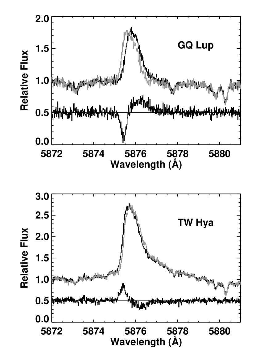
Figure 2.— In each panel, the continuum normalized right circularly polarized component of the He I 5876 Å line profile is shown in the upper black curve and the left circularly polarized component is shown in the gray curve. The difference (right – left) of the two, offset by 0.5, is shown in the lower black curve. This difference is $2\times$ Stokes $V$ with the profiles normalized in this way.

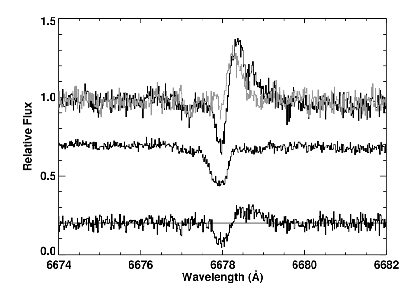
Figure 3.— The continuum normalized right circularly polarized component of the He I 6678 Å line profile of GQ Lup is shown in the upper black curve and the left circularly polarized component is shown in the gray curve. The difference (right – left) of the two, offset by 0.2, is shown in the bottom black curve. This difference is $2\times$ Stokes $V$ with the profiles normalized in this way. The middle black curve shows the same region in the Stokes $I$ spectrum of V2129 Oph, revealing the presence of a strong Fe I photospheric absorption line which can alter the inferred field in the He formation region if the Fe line is not properly accounted for.

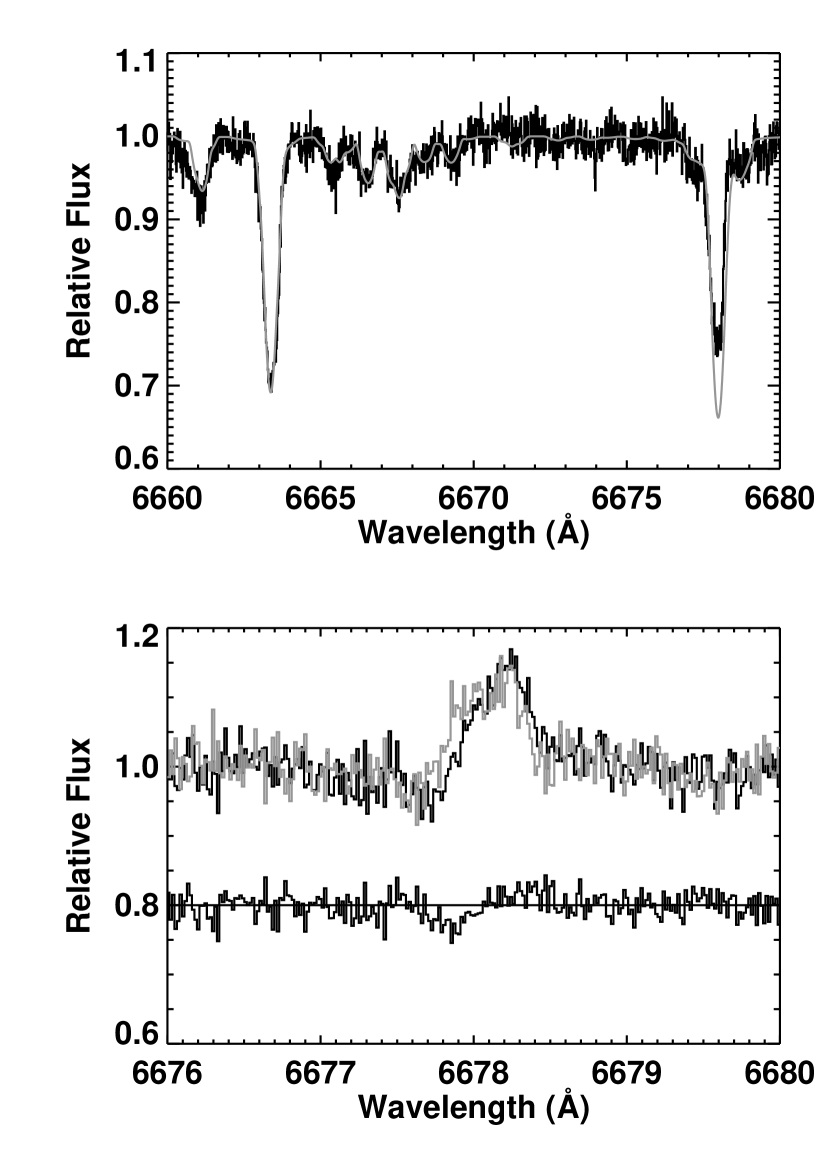
Figure 4.— The upper panel shows the observed Stokes $I$ spectrum of V2129 Oph in an expanded region near the He I 6678 Å line. The two strongest lines are Fe I lines at 6678 Å and 6663 Å. The smooth gray curve in the upper panel shows a synthetic fit to the spectrum, showing that there is excess emission the spectrum of V2129 Oph at 6678 Å due to a weak He I emission line superimposed on the photospheric absorption spectrum. In the bottom panel, the upper black curve shows the continuum normalized right circularly polarized component of the He I 6678 Å line profile of V2129 Oph after subtracting off the synthetic fit and adding 1.0 back to the result. The gray curve shows the same for the left circularly polarized component of the spectrum. The difference (right – left) of the two, offset by 0.8, is shown in the lower black curve. This difference is $2\times$ Stokes $V$ with the profiles normalized in this way.

References

- (1) Alencar, S. H. P., & Basri, G. 2000, AJ, 119, 1881
- (2) Alencar, S. H. P., & Batalha, C. 2002, ApJ, 571, 378
- (3) Alencar, S. H. P., Johns–Krull, C. M., & Basri, G., 2001, AJ, 122, 3335
- (4) Allard, F. & Hauschildt, P.H. 1995, in Bottom of the Main Sequence and Beyond, ed. C.G. Tinney (Berlin: Springer), 32
- (5) Asensio Ramos, A., Trujillo Bueno, J., & Landi Degl’Innocenti, E. 2008, ApJ, 683, 542
- (6) Azevedo, R., Calvet, N., Hartmann, L., Folha, D. F. M., Gameiro, F., & Muzerolle, J. 2006, A&A, 456, 225
- (7) Babcock, H. W. 1962, in Astronomical Techniques, ed. W. A. Hiltner (Chicago: Univ. of Chicago Press), p. 107
- (8) Bagnulo, S., Landolfi, M., Landstreet, J. D., Landi Degl Innocenti, E., Fossati, L., & Sterzik, M. 2009, PASP, 121, 993
- (9) Basri, G., & Batalha, C. 1990, ApJ, 363, 654
- (10) Basri, G., Marcy, G. W., & Valenti, J. A. 1992, ApJ, 390, 622
- (11) Batalha, C., Lopes, D. F., & Batalha, N. M. 2001, ApJ, 548, 377
- (12) Batalha, C. C., Stout–Batalha, N. M., Basri, G., & Terra, M. A. O. 1996, ApJS, 103, 211
- (13) Beristain, G., Edwards, S., & Kwan, J. 2001, ApJ, 551, 1037
- (14) Bertout, C. 1989, ARAA, 27, 351
- (15) Bertout, C., Basri, G., & Bouvier, J. 1988, ApJ, 330, 350
- (16) Bertout, C., Harder, S., Malbet, F., Mennessier, C., & Regev, O. 1996, AJ, 112, 2159
- (17) Borra, E. F. & Vaughan, A. H. 1977, ApJ, 216, 462
- (18) Bouvier, J., et al. 1999, A&A, 349, 619
- (19) Bouvier, J., Alencar, S. H. P., Harries, T. J., Johns-Krull, C. M., & Romanova, M. M. 2007, Protostars and Planets V, 479
- (20) Calvet, N., & Gullbring, E. 1998, ApJ, 509, 802
- (21) Camenzind, M. 1990, Rev. Modern Astron., (Berlin: Springer-Verlag), 3, 234
- (22) Cauley, P. W., Johns-Krull, C. M., Hamilton, C. M., & Lockhart, K. 2012, ApJ, 756, 68
- (23) Chen, W. & Johns–Krull, C.M. 2011, ASP Conf. Series, in press
- (24) Collier Cameron, A. & Campbell, C. G. 1993, A&A, 274, 309
- (25) Daou, A. G., Johns–Krull, C. M., & Valenti, J. A. 2006, AJ, 131, 520
- (26) Donati, J.-F., Semel, M., Carter, B. D., Rees, D. E., & Collier Cameron, A. 1997, MNRAS, 291, 658
- (27) Donati, J.-F., et al. 2007, MNRAS, 380, 1297
- (28) Donati, J.-F., et al. 2008, MNRAS, 386, 1234
- (29) Donati, J.-F., et al. 2010a, MNRAS, 402, 1426
- (30) Donati, J.-F., et al. 2010b, MNRAS, 409, 1347
- (31) Donati, J.-F., et al. 2011a, MNRAS, 412, 2454
- (32) Donati, J.-F., et al. 2011b, MNRAS, 417, 472
- (33) Donati, J.-F., et al. 2012, MNRAS, 425, 2948
- (34) Edwards, S., Hartigan, P., Ghandour, L., & Andrulis, C. 1994, AJ, 108, 1056
- (35) Feigelson, E. D. & Montmerle, T. 1999, ARAA, 37, 363
- (36) Ferreira, J. 2008, New Astronomy Review, 52, 42
- (37) Gregory, S. G., Matt, S. P., Donati, J.-F., & Jardine, M. 2008, MNRAS, 389, 1839
- (38) Guenther, E. W., Lehmann, H., Emerson, J. P., & Staude, J. 1999, A&A, 341, 768
- (39) Guenther, E. W., Neuhäuser, R., Wuchterl, G., et al. 2005, Astronomische Nachrichten, 326, 958
- (40) Gullbring, E., Hartmann, L., Briceño, C., & Calvet, N. 1998, ApJ, 492, 323
- (41) Hartigan, P., Edwards, S., & Ghandour, L. 1995, ApJ, 452, 736
- (42) Hartigan, P., Kenyon, S. J., Hartmann, L., Strom, S. E., Edwards, S., Welty, A. D., & Stauffer, J. 1991, ApJ, 382, 617
- (43) Hartmann, L., Hewett, R., & Calvet, N. 1994, ApJ, 426, 669
- (44) Herbig, G. H., & Bell, K. R. 1988, Third catalog of emission-line stars of the Orion population., by G.H. gerbig and K.R. Bell. Lick Observatory Bulletin #1111, Santa Cruz: Lick Observatory, Jun 1988, 90 p.
- (45) Herbst, W., Bailer–Jones, C. A. L., & Mundt, R. 2001, ApJ, 554, L197
- (46) Hinkle, K., Wallace, L., Valenti, J., & Harmer, D. 2000, Visible and Near Infrared Atlas of the Arcturus Spectrum 3727-9300 A ed. Kenneth Hinkle, Lloyd Wallace, Jeff Valenti, and Dianne Harmer. (San Francisco: ASP) ISBN: 1-58381-037-4, 2000.,
- (47) Huélamo, N., Figueira, P., Bonfils, X., et al. 2008, A&A, 489, L9
- (48) Hussain, G. A. J., et al. 2009, MNRAS, 398, 189
- (49) Jayawardhana, R., Mohanty, S., & Basri, G. 2003, ApJ, 592, 282
- (50) Johns, C. M. & Basri, G. 1995, ApJ, 449, 341
- (51) Johns–Krull, C. M. 2007, ApJ, 664, 975
- (52) Johns–Krull, C. M. & Gafford, A. D. 2002, ApJ, 573, 685
- (53) Johns–Krull, C. M., Valenti, J. A., Hatzes, A. P., & Kanaan, A. 1999a, 510, L41
- (54) Johns–Krull, C. M., Valenti, J. A., & Koresko, C. 1999b, ApJ, 516, 900
- (55) Johns–Krull, C. M., Valenti, J. A., & Saar, S. H. 2004, ApJ, 617, 1204
- (56) Kastner, J. H., Zuckerman, B., Weintraub, D. A., & Forveille, T. 1997, Science, 277, 67
- (57) Königl, A. 1991, ApJ, 370, L39
- (58) Kenyon, S. J., Hartmann, L., Hewett, R., Carrasco, L., Cruz–Gonzalez, I., Recillas, E., Salas, L., Serrano, A., Strom, K. M., Strom, S. E., & Newton, G. 1994, AJ, 107, 2153
- (59) Kochukhov, O., Bagnulo, S., Wade, G. A., Sangalli, L., Piskunov, N., Landstreet, J. D., Petit, P., & Sigut, T. A. A. 2004, A&A, 414, 613
- (60) Kochukhov & Wade 2010, A&A, 513, 13
- (61) Kupka, F., Ryabchikova, T.A., Piskunov, N.E., Stempels, H.C., & Weiss, W.W., 2000, Baltic Astronomy, vol. 9, 590
- (62) Kupka, F., Piskunov, N.E., Ryabchikova, T.A., Stempels H.C., & Weiss, W.W., 1999, A&AS 138, 119
- (63) Kurucz, R. L., Furenlid, I., Brault, J., & Testerman, L. 1984, National Solar Observatory Atlas, Sunspot, New Mexico: National Solar Observatory, 1984
- (64) Lamzin, S. A. 1998, Astronomy Reports, 42, 322
- (65) Landi Degl Innocenti E. & Landolfi, M., 2004, Polarisation in Spectral Lines. Vol. 307 of Astrophysics and Space Science Library, Kluwer Academic Publishers
- (66) Long, M., Romanova, M. M., & Lovelace, R. V. E. 2005, ApJ, 634, 1214
- (67) Long, M., Romanova, M. M., & Lovelace, R. V. E. 2008, MNRAS, 386, 1274
- (68) Marois, C., Macintosh, B., & Barman, T. 2007, ApJ, 654, L151
- (69) Mathys, G. 1989, Fund. Cosmic Phys., 13, 143
- (70) Mathys, G. 1991, A&AS, 89, 121
- (71) Mayor, M., et al. 2003, The Messenger, 114, 20
- (72) McElwain, M. W., Metchev, S. A., Larkin, J. E., et al. 2007, ApJ, 656, 505
- (73) Mohanty, S., & Shu, F. H. 2008, ApJ, 687, 1323
- (74) Morin, J., Donati, J.-F., Petit, P., et al. 2008, MNRAS, 390, 567
- (75) Mugrauer, M., & Neuhäuser, R. 2005, Astronomische Nachrichten, 326, 701
- (76) Muzerolle, J., Calvet, N., Briceẽno, C., Hartmann, L., & Hillenbrand, L. 2000, ApJ, 535, L47
- (77) Muzerolle, J., Calvet, N., & Hartmann, L. 1998, ApJ, 492, 743
- (78) Muzerolle, J., Calvet, N., & Hartmann, L. 2001, ApJ, 550, 944
- (79) Neuhäuser, R., Guenther, E. W., Wuchterl, G., et al. 2005, A&A, 435, L13
- (80) Neuhäuser, R., Mugrauer, M., Seifahrt, A., Schmidt, T. O. B., & Vogt, N. 2008, A&A, 484, 281
- (81) Paatz, G. & Camenzind, M. 1996, A&A, 308, 77
- (82) Piskunov, N. 1999, Polarization, 243, 515
- (83) Piskunov, N. E., & Valenti, J. A. 2002, A&A, 385, 1095
- (84) Plachinda, S. I., & Tarasova, T. N. 1999, ApJ, 514, 402
- (85) Romanova, M. M., Long, M., Lamb, F. K., Kulkarni, A. K., & Donati, J.-F. 2011, MNRAS, 411, 915
- (86) Romanova, M. M., Ustyugova, G. V., Koldoba, A. V., & Lovelace, R. V. E. 2004, ApJ, 610, 920
- (87) Romanova, M. M., Ustyugova, G. V., Koldoba, A. V., & Lovelace, R. V. E. 2009, MNRAS, 399, 1802
- (88) Seifahrt, A., Neuhäuser, R., & Hauschildt, P. H. 2007, A&A, 463, 309
- (89) Seperuelo Duarte, E., Alencar, S. H. P., Batalha, C., & Lopes, D. 2008, A&A, 489, 349
- (90) Setiawan, J., Henning, T., Launhardt, R., et al. 2008, Nature, 451, 38
- (91) Shu, F. H., Najita, J., Ostriker, E., Wilkin, F., Ruden, S., & Lizano, S. 1994, ApJ, 429, 781
- (92) Siess, L., Dufour, E., & Forestini, M. 2000, A&A, 358, 593
- (93) Smirnov, D. A., Lamzin, S. A., Fabrika, S. N., & Chuntonov, G. A. 2004, Astronomy Letters, 30, 456
- (94) Snik, F., Jeffers, S., Keller, C., Piskunov, N., Kochukhov, O., Valenti, J., & Johns-Krull, C. 2008, Proc. SPIE, 7014
- (95) Snik, F., Kochukhov, O., Piskunov, N., et al. 2011, Solar Polarization 6, 437, 237
- (96) Stempels, H. C., & Piskunov, N. 2003, A&A, 408, 693
- (97) Symington, N. H., Harries, T. J., Kurosawa, R., & Naylor, T. 2005, MNRAS, 358, 977
- (98) Tull, R. G., MacQueen, P. J., Sneden, C., & Lambert, D. L. 1995, PASP, 107, 251
- (99) Valenti, J. A. 1994, Ph.D. Thesis, University of California, Berkeley
- (100) Valenti, J. A., Basri, G., & Johns, C. M. 1993, AJ, 106, 2024
- (101) Valenti, J. A. & Johns–Krull, C. M. 2004, Ap&SS, 292, 619
- (102) Valenti, J. A., & Piskunov, N. 1996, A&AS, 118, 595
- (103) Vink, J. S., Drew, J. E., Harries, T. J., Oudmaijer, R. D., & Unruh, Y. C. 2003, A&A, 406, 703
- (104) Vink, J. S., Harries, T. J., & Drew, J. E. 2005, A&A, 430, 213
- (105) Vogt, S. S. 1978, Ph.D. Thesis, The Univ. of Texas at Austin, Austin, TX
- (106) Vogt, S. S., Tull, R. G., & Kelton, P. W. 1980, ApJ, 236, 308
- (107) Webb, R. A., Zuckerman, B., Platais, I., et al. 1999, ApJ, 512, L63
- (108) Weise, P., Launhardt, R., Setiawan, J., & Henning, T. 2010, A&A, 517, A88
- (109) White, R. J., & Basri, G. 2003, ApJ, 582, 1109
- (110) Wichmann, R., Bastian, U., Krautter, J., Jankovics, I., & Rucinski, S. M. 1998, MNRAS, 301, L39
- (111) Yang, H., & Johns-Krull, C. M. 2011, ApJ, 729, 83
- (112) Yang, H., Johns–Krull, C. M., & Valenti, J. A. 2005, ApJ, 635, 466
- (113) Yang, H., Johns–Krull, C. M., & Valenti, J. A. 2007, AJ, 133, 73
- (114) Yang, H., Johns-Krull, C. M., & Valenti, J. A. 2008, AJ, 136, 2286
- (115) Zanni, C., & Ferreira, J. 2009, A&A, 508, 1117