Substructuring Preconditioners for
an $h$-$p$ Nitsche-type method

Abstract

We propose and study an iterative substructuring method for an $h$-$p$ Nitsche-type discretization, following the original approach introduced in [18] for conforming methods. We prove quasi-optimality with respect to the mesh size and the polynomial degree for the proposed preconditioner. Numerical experiments asses the performance of the preconditioner and verify the theory.

1 Introduction

Discontinuous Galerkin (DG) Interior Penalty (IP) methods were introduced in the late 70’s for approximating elliptic problems. They were arising as a natural evolution or extension of Nitsche’s method [43], and were based on the observation that inter-element continuity could be attained by penalization; in the same spirit Dirichlet boundary conditions are weakly imposed for Nitsche’s method [43]. The use, study and application of DG IP methods was abandoned for a while, probably due to the fact that they were never proven to be more advantageous or efficient than their conforming relatives. The lack of optimal and efficient solvers for the resulting linear systems, at that time, surely was also contributing to that situation.

However, over the last 10-15 years, there has been a considerable interest in the development and understanding of DG methods for elliptic problems (see, for instance, [7] and the references therein), partly due to the simplicity with which the DG methods handle non-matching grids and allow for the design of hp-refinement strategies. The IP and Nitsche approaches have also found some new applications; in the design of new conforming and non-conforming methods [9, 8, 39, 25, 40, 38] and as a way to deal with non-matching grids for domain decomposition [14, 33].

This has also motivated the interest in developing efficient solvers for DG methods. In particular, additive Schwarz methods are considered and analyzed in [35, 20, 3, 4, 5, 6, 13, 20]. Multigrid methods are studied in [37, 21, 41]. Two-level methods and multi-level methods are presented in [27, 22] and other subspace correction methods are considered in [12, 10, 11].

Still the development of preconditioners for DG methods based on Domain Decomposition (DD) has been mostly limited to classical Schwarz methods. Research towards more sophisticated non-overlapping DD preconditioners, such as the BPS (Bramble Pasciak Schatz), Neuman-Neuman, BDDC, FETI or FETI-DP is now at its inception. Non-overlapping DD methods typically refer to methods defined on a decomposition of a domain made up of a collection of mutually disjoint subdomains, generally called substructures. These family of methods are obviously well suited for parallel computations and furthermore, for several problems (like problems with jump coefficients) they offer some advantages over their relative overlapping methods, and have already proved their usefulness. Roughly speaking, these methods are algorithms for preconditioning the Schur complement with respect to the unknowns on the skeleton of the subdomain partition. They are generally referred substructuring preconditioners.

While the theory for the confoming case is now well established and understood for many problems [51], the discontinuous nature of the finite element spaces at the interface of the substructures (in the case of Nitsche-type methods) or even within the skeleton of the domain partition, poses extra difficulties in the analysis which preclude from having a straight extension of such theory. Mainly, unlike in the conforming case, the coupling of the unknowns along the interface does not allow for splitting the global bilinear form as a sum of local bilinear forms associated to the substructures (see for instance [35] and [3, Proposition 3.2]). Moreover the discontinuity of the finite element space makes the use of standard $H^{1/2}$-norms in the analysis of the discrete harmonic functions difficult.

For Nitsche-type methods, a new definition of discrete harmonic function has been introduced in [29] together with some tools (similar to those used in the analysis of mortar preconditioners) that allow them to adapt and extend the general theory [51] for substructuring preconditioners in two dimensions. More precisely, in [29, 30, 31] the authors introduced and analyzed Balancing Domain with Constrains BDDC, Neuman-Neuman and FETI-DP domain decomposition preconditioners for a first order Nitsche type discretization of an elliptic problem with jumping coefficients. For the discretization, a symmetric IP DG scheme is used (only) on the skeleton of the subdomain partition, while piecewise linear conforming approximation is used in the interior of the subdomains. In these works, the authors prove quasi-optimality with respect to the mesh-size and optimality with respect to the jump in the coefficient. They also address the case of non-conforming meshes.

More recently, several BDDC preconditioners have been introduced and analyzed for some full DG discretizations [48, 23, 47], following a different path. In [48] the authors consider the $p$-version of the preconditioner for an Hibridized IP DG method [24, 34], for which the unknown is defined directly on the skeleton of the partition. They prove cubic logarithmic growth on the polynomial degree but also show numerically that the results are not sharp. The IP DG and the IP-spectral DG methods for an elliptic problem with jumping coefficient are considered in [47] and [23], respectively. In both works the approach for the analysis differs considerably from the one taken in [29, 30, 31] and relies on suitable space decomposition of the global DG space; using either nonconforming or conforming subspaces. This allow the authors to adapt the classical theories for analyzing the resulting BDDC preconditioners.

In this work, we focus on the original substructuring approach introduced in [18] for conforming discretization of two dimensional problems and in [19, 32] for three dimensions (see also [52, 51] for a detailed description). In the framework of non conforming domain decomposition methods, this kind of preconditioner has been applied to the mortar method [1, 16, 45, 46] and to the three fields domain decomposition method [15], always considering the $h$-version of the methods. For spectral discretizations and the $p$ version of conforming approximations the preconditioner has been studied in [44, 42]. For $h$-$p$ conforming discretizations of two dimensional problems the BPS preconditioner is studied in [2]. To the best of our knowledge, this preconditioner has not been considered for Nitsche or DG methods before.

Here, we propose a BPS (Bramble-Pasciak-Schatz) preconditioner for an $h$-$p$ Nitsche type discretization of elliptic problems. In our analysis, we use some of the tools introduced in [29, 30], such as their definition of the discrete harmonic lifting that allows for defining the discrete Steklov-Poincaré operator associated to the Nitsche-type method. However, our construction of the preconditioners is guided by the definition of a suitable norm on the skeleton of the subdomain partition, that scales like an $H^{1/2}$-norm and captures the energy of the DG functions on the skeleton. This allow us to provide a much simpler analysis, proving quasi-optimality with respect to the mesh size and the polynomial degree for the proposed preconditioners. Furthermore, we demonstrate that unlike what happens in the conforming case, to ensure quasi-optimality of the preconditioners a block diagonal structure that de-couples completely the edge and vertex degrees of freedom on the skeleton is not possible; this is due to the presence of the penalty term which is needed to deal with the discontinuity. We show however that the implementation of the preconditioner can be done efficiently and that it performs in agreement with the theory.

The rest of the paper is organized as follows. The basic notation, functional setting and the description of the Nitsche-type method are given in next section; Section 2. Some technical tools required in the construction and analysis of the proposed preconditioners are revised in Section 3. The substructuring preconditioner is introduced and analyzed in Section 4. Its practical implementation together with some variants of the preconditioner are discussed in Section 5. The theory is verified through several numerical experiments presented in Section 6. The proofs of some technical lemmas used in our analysis are reported in the Appendix A.

2 Nitsche methods and Basic Notation

In this section, we introduce the basic notation, the functional setting and the Nitsche discretization.

To ease the presentation we restrict ourselves to the following model problem. Let $\Omega\subset\mathbb{R}^{2}$ a bounded polygonal domain, let $f\in L^{2}(\Omega)$ and let

$$\left\{\begin{aligned} -\Delta u^{\ast}&=f\qquad&&\mbox{in }\Omega,\\ u^{\ast}&=0\qquad&&\mbox{on }\partial\Omega.\end{aligned}\right.$$

The above problem admits the following weak formulation: find $u^{*}\in H^{1}_{0}(\Omega)$ such that:

$$a(u^{*},v)=f(v)\qquad\text{ for all }v\in H^{1}_{0}(\Omega),$$ (1)

where

$$a(u,v)=\int_{\Omega}\nabla u\cdot\nabla v\,\textrm{dx}\qquad f(v)=\int_{\Omega}fv\,\textrm{dx}\;,\quad\forall\,u,v\in H^{1}_{0}(\Omega)$$

2.1 Partitions

We now introduce the different partitions needed in our work. We denote by ${\mathcal{T}}_{H}$ a subdomain partition of $\Omega$ into $N$ non-overlapping shape-regular triangular or quadrilateral subdomains:

$$\overline{\Omega}=\bigcup_{\ell=1}^{N}\overline{\Omega}_{\ell}, {\Omega_{\ell}}\cap\Omega_{j}=\emptyset \ell\neq j.$$

We set

$${H_{\ell}}=\min_{j\,:\,\bar{\Omega}_{\ell}\cap\bar{\Omega}_{j}\neq\emptyset}H_{\ell,j}\qquad\mbox{where }\quad H_{\ell,j}=\left|\partial{\Omega_{\ell}}\cap\partial\Omega_{j}\right|\;,$$ (2)

and we also assume that ${H_{\ell}}\simeq\mbox{diam}({\Omega_{\ell}})$ for each $\ell=1,\ldots N$. We finally define the granularity of ${\mathcal{T}}_{H}$ by $H=\min_{\ell}{H_{\ell}}$. We denote by $\Gamma$ and $\Gamma^{\partial}$ respectively the interior and the boundary portions of the skeleton of the subdomain partition ${\mathcal{T}}_{H}$:

$$\Gamma=\bigcup_{\ell=1}^{N}{\Gamma_{\ell}}, {\Gamma_{\ell}}=\partial{\Omega_{\ell}}\smallsetminus\partial\Omega \forall\,\ell=1,\ldots,N.$$

$$\Gamma^{\partial}=\bigcup_{\ell=1}^{N}{\Gamma^{\partial}_{\ell}}, {\Gamma^{\partial}_{\ell}}=:\partial{\Omega_{\ell}}\cap\partial\Omega \forall\,\ell=1\ldots,N.$$

We also define the complete skeleton as $\Sigma=\Gamma\cup\Gamma^{\partial}$. The edges of the subdomain partition that form the skeleton will be denoted by $E\subset\Gamma$ and we will refer to them as macro edges, if they do not allude to a particular subdomain or subdomain edges, when they do refer to a particular subdomain.

For each ${\Omega_{\ell}}$, let $\left\{{\mathcal{T}}_{h}^{\ell}\right\}$ be a family of fine partitions of $\Omega_{\ell}$ into elements (triangles or quadrilaterals) $K$ with diameter $h_{K}$. All partitions ${\mathcal{T}}_{h}^{\ell}$ are assumed to be shape-regular and we define a global partition ${\mathcal{T}}_{h}$ of $\Omega$ as

$${\mathcal{T}}_{h}=\bigcup_{\ell=1}^{N}{\mathcal{T}}_{h}^{\ell}.$$

Observe that by construction ${\mathcal{T}}_{h}$ is a fine partition of $\Omega$ which is compatible within each subdomain $\Omega_{\ell}$ but which may be non matching across the skeleton $\Gamma$. Throughout the paper, we always assume that the following bounded local variation property holds: for any pair of neighboring elements $K^{+}\in{\mathcal{T}}_{h}^{\ell^{+}}$ and $K^{-}\in{\mathcal{T}}_{h}^{\ell^{-}}$, $\ell^{+}\neq\ell^{-}$, $h_{K^{+}}\simeq h_{K^{-}}$.

Note that the restriction of ${\mathcal{T}}_{h}$ to the skeleton $\Gamma$ induces a partition of each subdomain edge $E\subset\Gamma$. We define the set of element edges on the skeleton $\Gamma$ and on the boundary of $\Omega$ as follows:

$${{\mathcal{E}}^{o}_{h}}: =\{e=\partial K^{+}\cap\partial K^{-}\cap\Gamma,\,K^{+}\in{\mathcal{T}}_{h}^{\ell^{+}}\,,K^{-}\in{\mathcal{T}}_{h}^{\ell^{-}}\,,\ell^{+}\neq\ell^{-}\}\,,$$

$${{\mathcal{E}}^{\partial}_{h}}: =\{e=\partial K\cap\partial\Omega,\,K\in{\mathcal{T}}_{h}\}\,,$$

and we set ${{\mathcal{E}}_{h}}={{\mathcal{E}}^{o}_{h}}\cup{{\mathcal{E}}^{\partial}_{h}}$. When referring to a particular subdomain, say ${\Omega_{\ell}}$ for some $\ell$, the set of element edges are denoted by

$${{\mathcal{E}}^{o,\ell}_{h}}=\{e\in{{\mathcal{E}}^{o}_{h}}:\ e\subset\partial{\Omega_{\ell}}\},\quad {{\mathcal{E}}^{\partial,\ell}_{h}}=\{e\in{{\mathcal{E}}^{\partial}_{h}}:\ e\subset\partial{\Omega_{\ell}}\},\quad {{\mathcal{E}}^{\ell}_{h}}={{\mathcal{E}}^{o,\ell}_{h}}\cup{{\mathcal{E}}^{\partial,\ell}_{h}}\;.$$

2.2 Basic Functional setting

For $s\geq 1$, we define the broken Sobolev space

$$H^{s}({\mathcal{T}}_{H})=\left\{\phi\in L^{2}(\Omega)\,\,:\quad\phi\big{|}_{{\Omega_{\ell}}}\in H^{s}({\Omega_{\ell}})\quad\forall\,\,{\Omega_{\ell}}\in{\mathcal{T}}_{H}\,\right\}\sim\prod_{\ell}\,H^{s}({\Omega_{\ell}})\;,$$

whereas the trace space associated to $H^{1}({\mathcal{T}}_{H})$ is defined by

$$\Phi=\prod_{\ell}\,H^{1/2}(\partial{\Omega_{\ell}}).$$

For $u=(u^{\ell})_{\ell=1}^{N}$ in $H^{1}({\mathcal{T}}_{H})$ we will denote by $u_{|_{\Sigma}}$ the unique element $\phi=(\phi^{\ell})_{\ell=1}^{N}$ in $\Phi$ such that

$$\phi^{\ell}=u^{\ell}_{|_{\partial{\Omega_{\ell}}}}.$$

We now recall the definition of some trace operators following [7], and introduce the different discrete spaces that will be used in the paper.

Let $e\in{{\mathcal{E}}^{o}_{h}}$ be an edge on the interior skeleton shared by two elements $K^{+}$ and $K^{-}$ with outward unit normal vectors ${\bf n}^{+}$ and ${\bf n}^{-}$, respectively. For scalar and vector-valued functions $\varphi\in H^{1}({\mathcal{T}}_{H})$ and ${\bf\tau}\in\left[{H}^{1}({\mathcal{T}}_{H})\right]^{2}$, we define the average and the jump on $e\in{{\mathcal{E}}^{o}_{h}}$ as

$$\{{\bf\tau}\}=\frac{1}{2}({\bf\tau}^{+}+{\bf\tau}^{-}), [\![\,\varphi\,]\!]=\varphi^{+}{\bf n}^{+}+\varphi^{-}{\bf n}^{-}\;, \mbox{on }e\in{{\mathcal{E}}^{o}_{h}}$$

On a boundary element edge $e\in{{\mathcal{E}}^{\partial}_{h}}$ we set $\{{\bf\tau}\}={\bf\tau}$ and $[\![\,\varphi\,]\!]=\varphi{\bf n}$, ${\bf n}$ denoting the outward unit normal vector to $\Omega$.

To each element $K\in\mathcal{T}^{\ell}_{h}$, we associate a polynomial approximation order $p_{K}\geq 1$, and define the $hp$-finite element space of piecewise polynomials as

$${X_{h}^{\ell}}=\{v\in C^{0}({\Omega_{\ell}})\text{~{}such~{}that~{}}v|_{K}\in\mathbb{P}^{p_{K}}(K),~{}K\in\mathcal{T}^{\ell}_{h}\},$$

where $\mathbb{P}^{p_{K}}(K)$ stands for the space of polynomials of degree at most $p_{K}$ on $K$. We also assume that the polynomial approximation order satisfies a local bounded variation property: for any pair of elements $K^{+}$ and $K^{-}$ sharing an edge $e\in{{\mathcal{E}}^{o}_{h}}$, $p_{K^{+}}\simeq p_{K^{-}}$.

Our global approximation space ${X_{h}}$ is then defined as

$${X_{h}}=\{v\in L^{2}(\Omega)\,\,:\text{~{}such~{}that~{}}v_{|_{{\Omega_{\ell}}}}\in{X_{h}^{\ell}}\}\sim\prod_{\ell=1}^{N}{X_{h}^{\ell}}\;,.$$

We also define ${X^{0}_{h}}\subset{X_{h}}$ as the subspace of functions of ${X_{h}}$ vanishing on the skeleton $\Sigma$, i.e.,

$${X^{0}_{h}}=\{v\in{X_{h}}\,\,:\text{~{}such~{}that~{}}v_{|_{\Sigma}}=0\}.$$

The trace spaces associated to ${X_{h}^{\ell}}$ and ${X_{h}}$ are defined as follows

$$\Phi_{h}^{\ell} =\{\eta^{\ell}\in H^{1/2}(\partial{\Omega_{\ell}})\,:\,\,\eta^{\ell}=w_{|_{\partial{\Omega_{\ell}}}}\text{ for some }w\in{X_{h}^{\ell}}\} \forall\ell=1,\ldots,N\;$$

$$\Phi_{h} =\prod_{\ell=1}^{N}\Phi_{h}^{\ell}\;\ \subset\Phi.$$

Notice that the functions in the above finite element spaces are conforming in the interior of each subdomain but are double-valued on $\Gamma$. Moreover, any function $v\in{X_{h}}$ can be represented as $v=(v^{\ell})_{\ell=1}^{N}$ with $v^{\ell}\in{X_{h}^{\ell}}$.

Next, for each subdomain ${\Omega_{\ell}}\in{\mathcal{T}}_{H}$ and for each subdomain edge $E\subset\partial{\Omega_{\ell}}$, we define the discrete trace spaces

$$\Phi_{\ell}(E)={\Phi_{h}^{\ell}}_{|_{E}}, \Phi^{o}_{\ell}(E)=\{\eta^{\ell}\in\Phi_{\ell}(E)\,\,:\;~{}~{}\eta^{\ell}=0\;\mbox{on }\partial E\,\}.$$

Note that, since we are in two dimensions, the boundary of a subdomain edge $E$ is the set of the two endpoints (or vertices) of $E$, that is if $E=(a,b)$ then $\partial E=\{a,b\}$.

Finally, we introduce a suitable coarse space ${\mathfrak{L}}_{H}\subset\Phi$, that will be required for the definition of the subtructuring preconditioner:

$${\mathfrak{L}}_{H}=\{\eta=(\eta^{\ell})\in\Phi\,\,:\,\,\,\eta^{\ell}_{|_{E}}\in\mathbb{P}^{1}(E),\quad\forall\,E\subset\partial{\Omega_{\ell}}\;,\,\,\,\forall{\Omega_{\ell}}\in{\mathcal{T}}_{H}\}\;.$$ (3)

2.3 Nitsche-type methods

In this section, we introduce the Nitsche-type method we consider for approximating the model problem (1). Here and in the following, to avoid the proliferation of constants, we will use the notation $x\lesssim y$ to represent the inequality $x\leq Cy$, with $C>0$ independent of the mesh size, of the polynomial approximation order, and of the size and number of subdomains. Writing $x\simeq y$ will signify that there exists a constant $C>0$ such that $C^{-1}x\leq y\leq Cx$.

We introduce the local mesh size function $\mathtt{h}\in L^{\infty}(\Sigma)$ defined as

$$\mathtt{h}(x)=\left\{\begin{aligned} &h_{K}\quad&&\textrm{if $x\in\partial K\cap\partial\Omega$},\\ &\min\{h_{K^{+}},h_{K^{-}}\}&&\textrm{if $x\in\partial K^{+}\cap\partial K^{-}\cap\Gamma$, $K^{\pm}\in{\mathcal{T}}_{h}^{\ell^{\pm}}\,,\ell^{+}\neq\ell^{-}$},\end{aligned}\right.$$ (4)

and the local polynomial degree function $\mathtt{p}\in L^{\infty}(\Sigma)$:

$$\mathtt{p}(x)=\left\{\begin{aligned} &p_{K}\quad&&\textrm{if $x\in\partial K\cap\partial\Omega$},\\ &\max\{p_{K^{+}},p_{K^{-}}\}&&\textrm{if $x\in\partial K^{+}\cap\partial K^{-}\cap\Gamma$, $K^{\pm}\in{\mathcal{T}}_{h}^{\ell^{\pm}}$, $\ell^{+}\neq\ell^{-}$}.\end{aligned}\right.$$ (5)

Remark 2.1.

A different definition for the local mesh size function $\mathtt{h}$ and the local polynomial degree function $\mathtt{p}$ involving harmonic averages is sometimes used for the definition of Nitsche or DG methods [29]. We point out that such a definition yields to functions $\mathtt{h}$ and $\mathtt{p}$ which are of the same order as the ones given in (4) and (5), and therefore result in an equivalent method.

We now define the following Nitsche-type discretization [50, 14] to approximate problem (1): find $u^{*}_{h}\in{X_{h}}$ such that

$${\mathcal{A}}_{h}(u^{*}_{h},v_{h})=f(v_{h})\qquad\text{ for all }v_{h}\in{X_{h}}\;,$$ (6)

where, for all $u,v\in{X_{h}}$, ${\mathcal{A}}_{h}(\cdot,\cdot)$ is defined as

$${\mathcal{A}}_{h}(u,v) =\sum_{\ell=1}^{N}\int_{{\Omega_{\ell}}}\nabla u\cdot\nabla v\,\textrm{dx}-\sum_{e\in{{\mathcal{E}}_{h}}}\int_{e}\{\nabla u\}\cdot[\![\,v\,]\!]\,\textrm{ds}$$ (7)

$$\quad-\sum_{e\in{{\mathcal{E}}_{h}}}\int_{e}[\![\,u\,]\!]\cdot\{\nabla v\}\,\textrm{ds}+\sum_{e\in{{\mathcal{E}}_{h}}}\alpha\,\int_{e}\mathtt{p}^{2}\,\mathtt{h}^{-1}[\![\,u\,]\!]\cdot[\![\,v\,]\!]\,\textrm{ds}.$$

Here, $\alpha>0$ is the penalty parameter that needs to be chosen $\alpha\geq\alpha_{0}$ for some $\alpha_{0}\gtrsim 1$ large enough to ensure the coercivity of ${\mathcal{A}}_{h}(\cdot,\cdot)$.

On ${X_{h}}$, we introduce the following semi-norms:

$$|v|_{1,{\mathcal{T}}_{H}}^{2}=\sum_{\ell=1}^{N}\|\nabla v\|^{2}_{L^{2}({\Omega_{\ell}})}, \qquad|v|_{\ast,{{\mathcal{E}}_{h}}}^{2} =\sum_{e\in{{\mathcal{E}}_{h}}}\|\mathtt{p}\,\mathtt{h}^{-1/2}\,[\![\,v\,]\!]\|_{L^{2}(e)}^{2},$$ (8)

together with the natural induced norm by $\mathcal{A}_{h}(\cdot,\cdot)$:

$$\|v\|_{\mathcal{A}}^{2}=|v|_{1,{\mathcal{T}}_{H}}^{2}+\alpha|v|_{\ast,{{\mathcal{E}}_{h}}}^{2} \forall\,v\in{X_{h}}\;.$$ (9)

Following [50] (see also [7]) it is easy to see the bilinear form ${\mathcal{A}}_{h}(\cdot,\cdot)$ is continuous and coercive (provided $\alpha\geq\alpha_{0}$ ) with respect the norm (9), i.e.,

$$\textrm{Continuitiy}: |{\mathcal{A}}_{h}(u,v)|\lesssim\|u\|_{\mathcal{A}}\|v\|_{\mathcal{A}} \forall\,u,v\in{X_{h}}$$

$$\textrm{Coercivity}: {\mathcal{A}}_{h}(v,v)\gtrsim\|v\|_{\mathcal{A}}^{2} \forall\,v\in{X_{h}}.$$

From now on we will always assume that $\alpha\geq\alpha_{0}$. Notice that the continuity and coercivity constants depend only on the shape regularity of ${\mathcal{T}}_{h}$.

3 Some technical tools

We now revise some technical tools that will be required in the construction and analysis of the proposed preconditioners.

We recall the local inverse inequalities (cf. [49], for example): for any $\eta\in\mathbb{P}^{p_{K}}(K)$ it holds

$$|\eta|_{H^{r}(e)}\lesssim p_{K}^{2(r-s)}h_{K}^{s-r}|\eta|_{H^{s}(e)},\qquad e\subset\partial K$$

for all $s,r$ with $0\leq s<r\leq 1$. Using the above inequality for $s=0$ and space interpolation, it is easy to deduce that for a subdomain edge $E\subset\partial\Omega_{\ell}$ and for all $s,r$, $0\leq s<r<1$, for all $\eta\in X_{h}^{\ell}|_{E}$ it holds that

$$|\eta|_{H^{r}(E)} \lesssim\max_{\begin{subarray}{c}K\in{\mathcal{T}}_{h}^{\ell}\\ \partial K\cap E\neq\emptyset\end{subarray}}(p_{K}^{2}h_{K}^{-1})^{(r-s)}|\eta|_{H^{s}(e)}\lesssim p_{\ell}^{2(s-r)}h_{\ell}^{s-r}|\eta|_{H^{s}(E)},$$ (10)

$$|\eta|_{H^{r}(\partial{\Omega_{\ell}})} \lesssim\max_{\begin{subarray}{c}K\in{\mathcal{T}}_{h}^{\ell}\\ \partial K\cap\partial{\Omega_{\ell}}\neq\emptyset\end{subarray}}(p_{K}^{2}h_{K}^{-1})^{(r-s)}|\eta|_{H^{s}(E)}\lesssim p_{\ell}^{2(r-s)}h_{\ell}^{s-r}|\eta|_{s,\partial{\Omega_{\ell}}},$$ (11)

where $h_{\ell}$ and $p_{\ell}$ refer to the minimum (resp. the maximum) of the restriction to $\partial{\Omega_{\ell}}$ of the local mesh size $\mathtt{h}$ (resp. the local polynomial degree function $\mathtt{p}$), that is,

$$h_{\ell}=\min_{x\in\partial{\Omega_{\ell}}\cap\Gamma}\mathtt{h}(x)\quad\text{and}\quad p_{\ell}=\max_{x\in\partial{\Omega_{\ell}}\cap\Gamma}\mathtt{p}(x).$$ (12)

We write conventionally

$$\frac{H\,p^{2}}{h}=\max_{\ell}\left\{\frac{H_{\ell}\,p_{\ell}^{2}}{h_{\ell}}\right\}.$$ (13)

The next two results generalize [18, Lemma 3.2, 3.4 and 3.5] and [15, Lemma 3.2] to the $hp$-version. The detailed proofs are reported in the Appendix A.

Lemma 3.1.

Let $\eta=(\eta^{\ell})_{\ell=1}^{N}\in\Phi_{h}$ and let $\chi=(\chi^{\ell})_{\ell=1}^{N}\in{\mathfrak{L}}_{H}$ be such that $\chi^{\ell}(a)=\eta^{\ell}(a)$ at all vertices $a$ of ${\Omega_{\ell}}$, for all ${\Omega_{\ell}}\in{\mathcal{T}}_{H}$. Then

$$\sum_{{\Omega_{\ell}}\in{\mathcal{T}}_{H}}|\chi^{\ell}|_{H^{1/2}(\partial{\Omega_{\ell}})}^{2}\lesssim\left(1+\log{\left(\frac{H\,p^{2}}{h}\right)}\right)\sum_{{\Omega_{\ell}}\in{\mathcal{T}}_{H}}|\eta^{\ell}|^{2}_{H^{1/2}(\partial{\Omega_{\ell}})}\;.$$

Lemma 3.2.

Let $\xi\in\Phi_{h}^{\ell}$ such that $\xi(a)=0$ at all vertices $a$ of ${\Omega_{\ell}}$. Let $\zeta_{L}\in H^{1/2}(\partial{\Omega_{\ell}})$ be linear on each subdomain edge of $\partial{\Omega_{\ell}}$. Then, it holds

$$\sum_{E\subset\partial{\Omega_{\ell}}}\|\xi\|_{H^{1/2}_{00}(E)}^{2}\lesssim\left(1+\log{\left(\frac{H_{\ell}\,p_{\ell}^{2}}{h_{\ell}}\right)}\right)^{2}\left|\xi+\zeta_{L}\right|_{H^{1/2}(\partial{\Omega_{\ell}})}^{2}\;,$$

where $h_{\ell}$ and $p_{\ell}$ are defined in (12) and $H_{\ell}$ is defined as in (2).

3.1 Norms on $\Phi_{h}$

We now introduce a suitable norm on $\Phi_{h}$ that will suggest how to properly construct the preconditioner. The natural norm that we can define for all $\eta=(\eta_{\ell})_{\ell}\in\Phi_{h}$ is:

$$\lVert\eta\rVert_{\Phi_{h}}=\inf_{\begin{array}[]{c}u\in{X_{h}}\\ {u}_{|\Sigma}=\eta\end{array}}\|u\|_{\mathcal{A}}\;,$$ (14)

where the $\inf$ is taken over all $u\in{X_{h}}$ that coincide with $\eta$ along $\Sigma$. We recall that since on $\Gamma$ both $u$ and $\eta$ are double valued, the identity $\eta=u_{|_{\Sigma}}$ is to be intended as $\eta^{\ell}=u^{\ell}_{|_{\partial{\Omega_{\ell}}}}$. Although (14) is the natural trace norm induced on $\Phi$ by the norm (9), working with it might be difficult.

For this reason, we introduce another norm which will be easier to deal with and which, as we will show below, is equivalent to (14). The structure of the preconditioner proposed in this paper will be driven by this norm. We define:

$$\lVert\eta\rVert_{\Phi_{h},*}^{2} =\sum_{{\Omega_{\ell}}\in{\mathcal{T}}_{H}}|\eta|^{2}_{H^{1/2}(\partial{\Omega_{\ell}})}+\alpha\sum_{e\in{{\mathcal{E}}_{h}}}\|\mathtt{p}\,\mathtt{h}^{-1/2}[\![\,\eta\,]\!]\|_{L^{2}(e)}^{2}.$$ (15)

The next result shows that the norms (14) and (5.2) are indeed equivalent:

Lemma 3.3.

The following norm equivalence holds:

$$\lVert\eta\rVert_{\Phi_{h}}\lesssim\lVert\eta\rVert_{\Phi_{h},*}\lesssim\lVert\eta\rVert_{\Phi_{h}} \forall\eta\in\Phi_{h}$$

Proof.

We first prove that $\lVert\eta\rVert_{\Phi_{h},*}\lesssim\lVert\eta\rVert_{\Phi_{h}}$. Let $\eta=(\eta_{\ell})_{\ell=1,\dots,N}\in\Phi_{h}$ and let $u=(u_{\ell})_{\ell=1,\dots,N}$ such that ${u}_{|{\Sigma}}=\eta$ arbitrary. Thanks to the trace inequality, we have

$$|\eta_{\ell}|^{2}_{H^{1/2}(\partial{\Omega_{\ell}})}\lesssim|u_{\ell}|^{2}_{H^{1}({\Omega_{\ell}})}\;,$$

and so, summing over all the subdomains ${\Omega_{\ell}}\in{\mathcal{T}}_{H}$ we have

$$\sum_{{\Omega_{\ell}}\in{\mathcal{T}}_{H}}|\eta_{\ell}|^{2}_{H^{1/2}(\partial{\Omega_{\ell}})}\lesssim\sum_{{\Omega_{\ell}}\in{\mathcal{T}}_{H}}|u_{\ell}|^{2}_{H^{1}({\Omega_{\ell}})}=|u|_{1,{\mathcal{T}}_{H}}^{2}\;.$$

Adding now the term $\alpha\sum_{e\in{{\mathcal{E}}_{h}}}\|\mathtt{p}\mathtt{h}^{-1/2}[\![\,\eta\,]\!]\|_{L^{2}(e)}^{2}$ to both sides, and recalling the definition of the norms (9), (14) and (5.2) we get the thesis thanks to the arbitrariness of $u$.

We now prove that $\lVert\eta\rVert_{\Phi_{h}}\lesssim\lVert\eta\rVert_{\Phi_{h},*}$. Given $\eta=(\eta_{\ell})_{\ell=1,\dots,L}\in\Phi_{h}$ let $\check{u}_{\ell}\in X_{h}^{\ell}$ be the standard discrete harmonic lifting of $\eta^{\ell}$, for which the bound $|\check{u}_{\ell}|_{H^{1}({\Omega_{\ell}})}\lesssim|\eta_{\ell}|_{H^{1/2}(\partial{\Omega_{\ell}})}$ holds (see e.g. [18]) and let $\check{u}=(\check{u}^{\ell})_{\ell=1,\dots,L}$ Summing over all the subdomains ${\Omega_{\ell}}$ and adding the term $\alpha\sum_{e\in{{\mathcal{E}}_{h}}}\|\mathtt{p}\mathtt{h}^{-1/2}[\![\,\eta\,]\!]\|_{L^{2}(e)}^{2}$ we get

$$\lVert\eta\rVert_{\Phi_{h}}\leq\|\check{u}\|_{\mathcal{A}}\lesssim\lVert\eta\rVert_{\Phi_{h},*}.$$

∎

4 Substructuring preconditioners

In this section we present the construction and analysis of a substructing preconditioner for the Nitsche method (6)-(7).

The first step in the construction is to split the set of degrees of freedom into interior degrees of freedom (corresponding to basis functions identically vanishing on the skeleton) and degrees of freedom associated to the skeleton $\Gamma$ of the subdomain partition. Then,the idea of the “substructuring” approach (see [18]) consists in further distinguishing two types among the degrees of freedom associated to $\Gamma$ : edge degrees of freedom and vertex degrees of freedom. Therefore, any function $u\in{X_{h}}$ can be split as the sum of three suitably defined components: $u=u^{0}+u_{\Gamma}=u^{0}+u^{E}+u^{V}$.

We first show how to eliminate (or condensate) the interior degrees of freedom and introduce the discrete Steklov-Poincaré operator associated to (7), acting on functions living on the skeleton of the subdomain partition. We then propose a preconditioner of substructuring type for the discrete Steklov-Poincaré operator and provide the convergence analysis.

4.1 Discrete Steklov-Poincarè operator

Following [29, 30], we now introduce a discrete harmonic lifting that allows for defining the discrete Steklov-Poincaré operator associated to (7). We also show that such a discrete Steklov-Poincaré operator defines a norm that is equivalent to the one defined in (5.2).

Let ${X^{0}_{h}}\subset{X_{h}}$ be the subspace of functions vanishing on the skeleton of the decomposition. Given any discrete function $w\in{X_{h}}$, we can split it as the sum of an interior function $w^{0}\in{X^{0}_{h}}$ and a suitable discrete lifting of its trace. More precisely, following [29, 30], we split

$$w=w^{0}+R_{h}(w_{|\Sigma}),\qquad w^{0}\in{X^{0}_{h}},$$

where, for $\eta\in\Phi_{h}$, $R_{h}(\eta)\in{X_{h}}$ denotes the unique element of ${X_{h}}$ satisfying

$$R_{h}(\eta)_{|_{\Sigma}}=\eta,\quad {\mathcal{A}}_{h}(R_{h}(\eta),v_{h})=0 \forall v_{h}\in{X^{0}_{h}}.$$ (16)

The following proposition is easy to prove (see [29, 30]).

Proposition 4.1.

For $\eta=(\eta^{\ell})\in\Phi_{h}$, the following identity holds:

$$R_{h}(\eta)_{|_{{\Omega_{\ell}}}}=w_{\ell}^{H}+w_{\ell}^{0},$$

with $w_{\ell}^{H}\in X_{h}^{\ell}$ denoting the standard discrete harmonic lifting of $\eta^{\ell}$

$${w_{\ell}^{H}}=\eta^{\ell}\text{ on }\partial{\Omega_{\ell}},\quad \int_{\Omega_{\ell}}\nabla w_{\ell}^{H}\cdot\nabla v_{h}^{\ell}=0 \forall v_{h}^{\ell}\in X_{h}^{\ell}\cap H^{1}_{0}({\Omega_{\ell}}),$$

and $w_{\ell}^{0}\in X_{h}^{\ell}\cap H^{1}_{0}({\Omega_{\ell}})$ being the solution of

$$\int_{{\Omega_{\ell}}}\nabla w_{\ell}^{0}\cdot\nabla v_{h}^{\ell}=\int_{\partial{\Omega_{\ell}}}[\![\,\eta\,]\!]\cdot\nabla v_{h}^{\ell}, \forall v_{h}^{\ell}\in X_{h}^{\ell}\cap H^{1}_{0}({\Omega_{\ell}}).$$

The space ${X_{h}}$ can be split as direct sums of an interior and a trace component, that is

$${X_{h}}={X^{0}_{h}}\oplus R_{h}(\Phi_{h}).$$

Using the above splitting, the definition of $R_{h}(\cdot)$ and the definition of ${\mathcal{A}}_{h}(\cdot,\cdot)$, it is not difficult to verify that,

$${\mathcal{A}}_{h}(w,v) ={\mathcal{A}}_{h}(w^{0},v^{0})+{\mathcal{A}}_{h}(R_{h}(w_{|_{\Sigma}}),R_{h}(v_{|_{\Sigma}}))$$

$$=a(w^{0},v^{0})+s(w_{|_{\Sigma}},v_{|_{\Sigma}}),\qquad\qquad\forall\,w,v\in{X_{h}}$$

where the discrete Steklov-Poincaré operator $s:\Phi_{h}\times\Phi_{h}\to{\mathbb{R}}$ is defined as

$$s(\xi,\eta)={\mathcal{A}}_{h}(R_{h}(\xi),R_{h}(\eta))\qquad\forall\,\xi,\eta\in\Phi_{h}\;.$$ (17)

We have the following result:

Lemma 4.2.

Let $R_{h}$ be the discrete harmonic lifting defined in (16). Then,

$$\|R_{h}(\eta)\|_{\mathcal{A}}\simeq\lVert\eta\rVert_{\Phi_{h},*}\qquad\forall\,\eta\in\Phi_{h}\;.$$

Proof.

If we show that $\|R_{h}(\eta)\|_{\mathcal{A}}\simeq\lVert\eta\rVert_{\Phi_{h}}$, then the thesis follows thanks to the equivalence of the norms shown in Lemma 3.3. First, we prove that $\|R_{h}(\eta)\|_{\mathcal{A}}\lesssim\lVert\eta\rVert_{\Phi_{h}}$; let $\eta\in\Phi_{h}$, then from the definition of the $\inf$, we get that

$$\exists u\in{X_{h}}\,:\,u_{|\Sigma}=\eta\quad\mbox{ such that }\quad\|u\|_{\mathcal{A}}\leq 2\lVert\eta\rVert_{\Phi_{h}}\;.$$

Then, we can write $R_{h}(\eta)=u+v$ with $v\in{X^{0}_{h}}$, and (16) reads

$${\mathcal{A}}_{h}(v,w)=-{\mathcal{A}}_{h}(u,w)\qquad\forall w\in{X^{0}_{h}}\;.$$

Setting $w=v\in{X^{0}_{h}}$ in the above equation, leads to

$${\mathcal{A}}_{h}(v,v)=-{\mathcal{A}}_{h}(u,v)\;.$$

Then, using the coercivity and continuity of ${\mathcal{A}}_{h}(\cdot,\cdot)$ in the $\|\cdot\|_{\mathcal{A}}$-norm we find

$$\|v\|_{\mathcal{A}}^{2}\lesssim{\mathcal{A}}_{h}(v,v)=|{\mathcal{A}}_{h}(u,v)|\lesssim\|u\|_{\mathcal{A}}\|v\|_{\mathcal{A}}\;.$$

Hence, $\|v\|_{\mathcal{A}}\lesssim\|u\|_{\mathcal{A}}$, and so this bound together with the triangle inequality gives

$$\|R_{h}(\eta)\|_{\mathcal{A}}\leq\|u\|_{\mathcal{A}}+\|v\|_{\mathcal{A}}\lesssim\|u\|_{\mathcal{A}}\lesssim\lVert\eta\rVert_{\Phi_{h}}\;.$$

The other inequality $\lVert\eta\rVert_{\Phi_{h}}\lesssim\|R_{h}(\eta)\|_{\mathcal{A}}$ follows from the trace theorem. ∎

From the above result, the following result for the discrete Steklov-Poincarè operator follows easily.

Corollary 4.3.

For all $\xi\in\Phi_{h}$, it holds

$$s(\xi,\xi)\simeq\lVert\xi\rVert_{\Phi_{h},*}^{2}.$$

Proof.

Let $\xi\in\Phi_{h}$ then from the definition of $s(\cdot,\cdot)$, the continuity and coercivity of ${\mathcal{A}}_{h}(\cdot,\cdot)$ and applying Lemma 4.2 we have

$$s(\xi,\xi)={\mathcal{A}}_{h}(R_{h}(\xi),R_{h}(\xi))\simeq\|R_{h}(\xi)\|_{\mathcal{A}}^{2}\simeq\lVert\xi\rVert_{\Phi_{h},*}^{2}.$$

∎

4.2 The preconditioner

Following the approach introduced in [18], we now present the construction of a preconditioner for the discrete Steklov-Poincaré operator given by $s(\cdot,\cdot)$. We split the space of skeleton functions $\Phi_{h}$ as the sum of vertex and edge functions. We start by observing that ${\mathfrak{L}}_{H}\subset\Phi_{h}$. We then introduce the space of edge functions $\Phi_{h}^{E}\subset\Phi_{h}$ defined by

$$\Phi_{h}^{E}=\{\eta\in\Phi_{h},~{}\eta_{\ell}(A)=0~{}\text{ ~{}at all vertex $A$ of}~{}{\Omega_{\ell}}\quad\forall\,{\Omega_{\ell}}\in{\mathcal{T}}_{H}\}$$

and we immediately get

$$\Phi_{h}={\mathfrak{L}}_{H}\oplus\Phi_{h}^{E}.$$ (18)

The preconditioner ${\hat{s}}(\cdot,\cdot)$ that we consider is built by introducing bilinear forms

$${\hat{s}}^{E}:\Phi_{h}^{E}\times\Phi_{h}^{E}\longrightarrow{\mathbb{R}} \qquad{\hat{s}}^{V}:{\mathfrak{L}}_{H}\times{\mathfrak{L}}_{H}\longrightarrow{\mathbb{R}}$$

acting respectively on edge and vertex functions, satisfying

$${\hat{s}}^{E}(\eta^{E},\eta^{E}) \simeq\sum_{{\Omega_{\ell}}\in{\mathcal{T}}_{H}}\sum_{E\subset\partial{\Omega_{\ell}}}\|\eta^{E}\|^{2}_{H^{1/2}_{00}(E)} \forall\,\eta^{E}\in\Phi_{h}^{E},$$ (19)

$${\hat{s}}^{V}(\eta^{V},\eta^{V}) \simeq\sum_{{\Omega_{\ell}}\in{\mathcal{T}}_{H}}\left|\eta^{V}\right|^{2}_{H^{1/2}(\partial{\Omega_{\ell}})} \forall\,\eta^{V}\in{\mathfrak{L}}_{H},$$ (20)

and we define ${\hat{s}}:\Phi_{h}\times\Phi_{h}\longrightarrow{\mathbb{R}}$ as

$${\hat{s}}(\eta,\xi)={\hat{s}}^{E}(\eta^{E},\xi^{E})+{\hat{s}}^{V}(\eta^{V},\xi^{V})+q(\eta,\xi),$$ (21)

where

$$q(\eta,\eta) =\alpha\sum_{e\in{{\mathcal{E}}_{h}}}\|\mathtt{p}\,\mathtt{h}^{-1/2}[\![\,\eta\,]\!]\|_{L^{2}(e)}^{2} \forall\,\eta\in\Phi_{h}\;.$$ (22)

Finally, we can state the main theorem of the paper.

Theorem 4.4.

Let $s(\cdot,\cdot)$ and ${\hat{s}}(\cdot,\cdot)$ be the bilinear forms defined in (17) and (21), respectively. Then, we have:

$$\left(1+\log\left(H\,p^{2}/h\right)\right)^{-2}{\hat{s}}(\eta,\eta)\lesssim s(\eta,\eta)\lesssim{\hat{s}}(\eta,\eta)\qquad\forall\,\eta\in\Phi_{h}\;.$$

The proof of Theorem 4.4 follows the analogous proofs given in [18, 15] for conforming finite element approximation. We give it here for completeness.

Proof.

We start proving that $s(\eta,\eta)\lesssim{\hat{s}}(\eta,\eta)$. Let $\eta\in\Phi_{h}$, then, $\eta=\eta^{V}+\eta^{E}$ with $\eta^{E}\in\Phi_{h}^{E}$ and $\eta^{V}\in{\mathfrak{L}}_{H}$. By using Corollary 4.3, as well as the properties (19)-(20) of the edge and vertex bilinear forms, and (22) of $q(\cdot,\cdot)$, we get

$$s(\eta,\eta) \lesssim\lVert\eta\rVert_{\Phi_{h},*}^{2}=\sum_{{\Omega_{\ell}}\in{\mathcal{T}}_{H}}|\eta^{E}+\eta^{V}|^{2}_{1/2,\partial\Omega_{\ell}}+\alpha\sum_{e\in{{\mathcal{E}}_{h}}}\|\mathtt{p}\,\mathtt{h}^{-1/2}[\![\,\eta\,]\!]\|_{L^{2}(e)}^{2}$$

$$\lesssim\sum_{{\Omega_{\ell}}\in{\mathcal{T}}_{H}}|\eta^{E}|^{2}_{1/2,\partial\Omega_{\ell}}+\sum_{{\Omega_{\ell}}\in{\mathcal{T}}_{H}}|\eta^{V}|^{2}_{1/2,\partial\Omega_{\ell}}+q(\eta,\eta)$$

$$\lesssim{\hat{s}}^{E}(\eta^{E},\eta^{E})+{\hat{s}}^{V}(\eta^{V},\eta^{V})+q(\eta,\eta),$$

and hence

$$s(\eta,\eta)\lesssim{\hat{s}}(\eta,\eta)\qquad\forall\,\eta\in\Phi_{h}\;.$$

We next prove the lower bound. We shall show that

$${\hat{s}}(\eta,\eta)\lesssim\left(1+\log\left(H\,p^{2}/h\right)\right)^{2}s(\eta,\eta)\qquad\forall\,\eta\in\Phi_{h}\;.$$ (23)

For $\eta\in\Phi_{h}$, we have $\eta=\eta^{V}+\eta^{E}$ with $\eta^{E}\in\Phi_{h}^{E}$ and $\eta^{V}\in{\mathfrak{L}}_{H}$. Then, from the definition of ${\hat{s}}(\cdot,\cdot)$ we have

$${\hat{s}}(\eta,\eta) ={\hat{s}}^{E}(\eta^{E},\eta^{E})+{\hat{s}}^{V}(\eta^{V},\eta^{V})+q(\eta,\eta)$$

$$\simeq\sum_{{\Omega_{\ell}}\in{\mathcal{T}}_{H}}\sum_{E\subset\partial{\Omega_{\ell}}}\|\eta^{E}\|^{2}_{H^{1/2}_{00}(E)}+\sum_{{\Omega_{\ell}}\in{\mathcal{T}}_{H}}\left|\eta^{V}\right|^{2}_{H^{1/2}(\partial{\Omega_{\ell}})}+\alpha\sum_{e\in{{\mathcal{E}}_{h}}}\|\mathtt{p}\,\mathtt{h}^{-1/2}[\![\,\eta\,]\!]\|_{L^{2}(e)}^{2}.$$

Appling Lemma 3.2 with $\chi=\eta^{E}$ and $\zeta_{L}=\eta^{V}$, we obtain

$$\sum_{{\Omega_{\ell}}\in{\mathcal{T}}_{H}}\sum_{E\subset\partial{\Omega_{\ell}}}\|\eta^{E}\|^{2}_{H^{1/2}_{00}(E)}\lesssim\sum_{{\Omega_{\ell}}\in{\mathcal{T}}_{H}}\left(1+\log\left(\frac{H_{\ell}\,p_{\ell}^{2}}{h_{\ell}}\right)\right)^{2}|\eta|^{2}_{H^{1/2}({\Omega_{\ell}})},$$

that is

$${\hat{s}}^{E}(\eta^{E},\eta^{E})\lesssim\left(1+\log\left(H\,p^{2}/h\right)\right)^{2}\sum_{{\Omega_{\ell}}\in{\mathcal{T}}_{H}}|\eta|^{2}_{H^{1/2}(\partial{\Omega_{\ell}})}.$$

To bound ${\hat{s}}^{V}(\eta^{V},\eta^{V})$, we apply Lemma 3.1 with $\chi^{\ell}=\eta^{V}$ and $\eta^{\ell}=\eta$, and we get

$${\hat{s}}^{V}(\eta^{V},\eta^{V})\lesssim\sum_{{\Omega_{\ell}}\in{\mathcal{T}}_{H}}|\eta^{V}|^{2}_{H^{1/2}(\partial{\Omega_{\ell}})}\lesssim\left(1+\log\left(H\,p^{2}/h\right)\right)\sum_{{\Omega_{\ell}}\in{\mathcal{T}}_{H}}|\eta|^{2}_{H^{1/2}(\partial{\Omega_{\ell}})},$$

and hence

$${\hat{s}}^{E}(\eta^{E},\eta^{E})+{\hat{s}}^{V}(\eta^{V},\eta^{V})\lesssim\left(1+\log\left(H\,p^{2}/h\right)\right)^{2}\sum_{{\Omega_{\ell}}\in{\mathcal{T}}_{H}}|\eta|^{2}_{H^{1/2}(\partial{\Omega_{\ell}})}.$$

Adding now the term $\alpha\sum_{e\in{{\mathcal{E}}_{h}}}\|\mathtt{p}\mathtt{h}^{-1/2}[\![\,\eta\,]\!]\|_{L^{2}(e)}^{2}$ to both sides and recalling the definition of $q(\cdot,\cdot)$ we have:

$${\hat{s}}(\eta,\eta) ={\hat{s}}^{E}(\eta^{E},\eta^{E})+{\hat{s}}^{V}(\eta^{V},\eta^{V})+q(\eta,\eta)$$

$$\lesssim\left(1+\log\left(H\,p^{2}/h\right)\right)^{2}\left(\sum_{{\Omega_{\ell}}\in{\mathcal{T}}_{H}}|\eta|^{2}_{H^{1/2}(\partial{\Omega_{\ell}})}+\alpha\sum_{e\in{{\mathcal{E}}_{h}}}\|\mathtt{p}\mathtt{h}^{-1/2}[\![\,\eta\,]\!]\|_{L^{2}(e)}^{2}\right)$$

$$=\left(1+\log\left(H\,p^{2}/h\right)\right)^{2}\lVert\eta\rVert_{\Phi_{h},*}^{2}.$$

Finally, using the equivalence norm given in Corollary 4.3, we reach (23) and the proof of the Theorem is completed.

∎

As a direct consequence of Theorem 4.4 we obtain the following estimate for the condition number of the preconditioned Schur complement.

Corollary 4.5.

Let ${\mathbf{S}}$ and ${\mathbf{P}}$ be the matrix representation of the bilinear forms $s(\cdot,\cdot)$ and ${\hat{s}}(\cdot,\cdot)$, respectively. Then, the condition number of ${\mathbf{P}}^{-1}{\mathbf{S}}$, $\kappa({\mathbf{P}}^{-1}{\mathbf{S}})$, satisfies

$$\kappa({\mathbf{P}}^{-1}{\mathbf{S}})\lesssim\left(1+\log\left(H\,p^{2}/h\right)\right)^{2}.$$ (24)

Unfortunately, the splitting (18) of $\Phi_{h}$ is not orthogonal with respect to the $\hat{s}(\cdot,\cdot)$-inner product given in (21), and therefore the preconditioner based on $\hat{s}(\cdot,\cdot)$ is not block diagonal, in contrast to what happens in the full conforming case. Furthermore the off-diagonal blocks in the preconditioner cannot be dropped without loosing the quasi-optimality. The reason is the presence of the $q(\cdot,\cdot)$ bilinear form in the definition (21), and the fact that the two components in the splitting (18) of $\Phi_{h}$ scale differently in the semi-norm that $q(\cdot,\cdot)$ defines. In fact, it is possible to show that, if for some constant $\kappa(h)$, it holds

$$\|\eta^{V}\|_{\Phi_{h},*}^{2}\leq\kappa(h)\|\eta\|_{\Phi_{h},*}^{2} \forall\eta=\eta^{V}+\eta^{E}\in\Phi_{h},$$ (25)

then such $\kappa(h)$ must verify $\kappa(h)\gtrsim H/h$, which implies that, if we were to use a fully block diagonal preconditioner based on the splitting (18) of $\Phi_{h}$ an estimate of the form (23) would no be longer true. In order to show this, consider linear finite elements on quasi uniform meshes with meshsize $h$ in all subdomains, and let $\eta=(\eta^{\ell})_{\ell}$ be the function identically vanishing in all subdomains but one, say $\Omega_{k}$, and let $\eta^{k}$ be equal to $1$ in a single vertex of $\Omega_{k}$ and zero at all other nodes. With this definition, we have $|[\![\,\eta\,]\!]|=|\eta^{k}|$ on $\partial\Omega_{k}$ and $[\![\,\eta\,]\!]=0$ on $\Sigma\setminus\partial\Omega^{k}$. Then, by a direct calculation, and recalling the definition of the semi-norm $|\cdot|_{\ast,{{\mathcal{E}}_{h}}}$ in (8), we easily see that

$$|\eta|^{2}_{\ast,{{\mathcal{E}}_{h}}}\simeq 1,\quad\mbox{ but }\qquad|\eta^{V}|^{2}_{\ast,{{\mathcal{E}}_{h}}}\simeq\frac{H_{k}}{h_{k}}$$

or equivalently

$$q(\eta^{V},\eta^{V})\simeq\frac{H_{k}}{h_{k}}\;,\qquad q(\eta,\eta)\simeq 1.$$ (26)

Therefore the energy of coarse interpolant $\eta^{V}$ exceeds that of $\eta$ by a factor of $H_{k}/h_{k}$. Hence, bounding $\eta^{V}$ alone in the $\|\cdot\|_{\Phi_{h},*}$-norm would result in an estimate of the type (25)

$$q(\eta^{V},\eta^{V})\lesssim\|\eta^{V}\|_{\Phi_{h},*}^{2}\lesssim\kappa(h)q(\eta,\eta),$$ (27)

which in view of (26) would imply

$$\kappa(h)\gtrsim\frac{H_{k}}{h_{k}}.$$

Remark 4.1.

We point out that the lack of the block-diagonal structure of the preconditioner associated to ${\hat{s}}(\cdot,\cdot)$ defined in (21), will not affect its computational efficiency, see Section 6.

5 Realizing the preconditioner

We start by deriving the matrix form of the discrete Steklov-Poincaré operator $s(\cdot,\cdot)$ defined in (17). We choose a Lagrangian nodal basis for the discrete space $X_{h}$, and we take care of numbering interior degrees of freedom first (grouped subdomain-wise), then edge degrees of freedom (grouped edge by edge and in such a way that the degrees of freedom corresponding to the common edge of two adjacent subdomains are ordered consecutively), and finally the degrees of freedom corresponding to the vertices of the subdomains. We let $\mathtt{n}_{\mathtt{i}}$, $\mathtt{n}_{\mathtt{e}}$ and $\mathtt{n}_{\mathtt{v}}$ be the number of interior, edge and vertex degrees of freedom, respectively, and set $\mathtt{n}=\mathtt{n}_{\mathtt{e}}+\mathtt{n}_{\mathtt{v}}$ Problem (6) is then reduced to looking for a vector ${{\mathbf{u}}}\in\mathbb{R}^{\mathtt{n}_{\mathtt{i}}+\mathtt{n}}$ with ${\mathbf{u}}=({\mathbf{u}}_{\mathtt{i}},{\mathbf{u}}_{\mathtt{e}},{\mathbf{u}}_{\mathtt{v}})$ solution to a linear system of the following form

$$\begin{pmatrix}{\mathbf{A}}_{\mathtt{i}\mathtt{i}}&{\mathbf{A}}_{\mathtt{i}\mathtt{e}}&{\mathbf{A}}_{\mathtt{i}\mathtt{v}}\\ {\mathbf{A}}_{\mathtt{i}\mathtt{e}}^{T}&{\mathbf{A}}_{\mathtt{e}\mathtt{e}}&{\mathbf{A}}_{\mathtt{e}\mathtt{v}}\\ {\mathbf{A}}_{\mathtt{i}\mathtt{v}}^{T}&{\mathbf{A}}_{\mathtt{e}\mathtt{v}}^{T}&{\mathbf{A}}_{\mathtt{v}\mathtt{v}}\end{pmatrix}\begin{pmatrix}{\mathbf{u}}_{\mathtt{i}}\\ {\mathbf{u}}_{\mathtt{e}}\\ {\mathbf{u}}_{\mathtt{v}}\end{pmatrix}=\begin{pmatrix}{\mathbf{F}}_{\mathtt{i}}\\ {\mathbf{F}}_{\mathtt{e}}\\ {\mathbf{F}}_{\mathtt{v}}\end{pmatrix}.$$

Here, ${\mathbf{u}}_{\mathtt{i}}\in\mathbb{R}^{\mathtt{n}_{\mathtt{i}}}$ (resp. ${\mathbf{F}}_{\mathtt{i}}\in\mathbb{R}^{\mathtt{n}_{\mathtt{i}}}$) represents the unknown (resp. the right hand side) component associated to interior nodes. Analogously, ${\mathbf{u}}_{\mathtt{e}},{\mathbf{F}}_{\mathtt{e}}\in\mathbb{R}^{\mathtt{n}_{\mathtt{e}}}$ and ${\mathbf{u}}_{\mathtt{v}},{\mathbf{F}}_{\mathtt{v}}\in\mathbb{R}^{\mathtt{n}_{\mathtt{v}}}$ are associated to edge and vertex nodes, respectively. We recall that for each vertex we have one degree of freedom for each of the subdomains sharing it. For each macro edge $E$, we will have two sets of nodes (some of them possibly physically coinciding) corresponding to the degrees of freedom of $\Phi_{h}^{\ell^{+}}(E)$ and of $\Phi_{h}^{\ell^{-}}(E)$.

As usual, we start by eliminating the interior degrees of freedom, to obtain the Schur complement system

$${\mathbf{S}}\begin{pmatrix}{\mathbf{u}}_{\mathtt{e}}\\ {\mathbf{u}}_{\mathtt{v}}\end{pmatrix}={\mathbf{g}},$$

with

$${\mathbf{S}}=\begin{pmatrix}{\mathbf{A}}_{\mathtt{e}\mathtt{e}}-{\mathbf{A}}_{\mathtt{i}\mathtt{e}}^{T}{\mathbf{A}}_{\mathtt{i}\mathtt{i}}^{-1}{\mathbf{A}}_{\mathtt{i}\mathtt{e}}&{\mathbf{A}}_{\mathtt{e}\mathtt{v}}-{\mathbf{A}}_{\mathtt{i}\mathtt{e}}^{T}{\mathbf{A}}_{\mathtt{i}\mathtt{i}}^{-1}{\mathbf{A}}_{\mathtt{i}\mathtt{v}}\\ {\mathbf{A}}_{\mathtt{e}\mathtt{v}}^{T}-{\mathbf{A}}_{\mathtt{i}\mathtt{v}}^{T}{\mathbf{A}}_{\mathtt{i}\mathtt{i}}^{-1}{\mathbf{A}}_{\mathtt{i}\mathtt{e}}&{\mathbf{A}}_{\mathtt{v}\mathtt{v}}-{\mathbf{A}}_{\mathtt{i}\mathtt{v}}^{T}{\mathbf{A}}_{\mathtt{i}\mathtt{i}}^{-1}{\mathbf{A}}_{\mathtt{i}\mathtt{v}}\end{pmatrix}, {\mathbf{g}}=\begin{pmatrix}{\mathbf{F}}_{E}-{\mathbf{A}}_{\mathtt{i}\mathtt{e}}^{T}{\mathbf{A}}_{\mathtt{i}\mathtt{i}}^{-1}{\mathbf{F}}_{\mathtt{i}}\\ {\mathbf{F}}_{V}-{\mathbf{A}}_{\mathtt{i}\mathtt{v}}^{T}{\mathbf{A}}_{\mathtt{i}\mathtt{i}}^{-1}{\mathbf{F}}_{\mathtt{i}}\end{pmatrix}.$$

The Schur complement ${\mathbf{S}}$ represents the matrix form of the Steklov-Poincaré operator $s(\cdot,\cdot)$. Remark that in practice we do not need to actually assemble ${\mathbf{S}}$ but only to be able to compute its action on vectors.

In order to implement the preconditioner introduced in the previous section we need to represent algebraically the splitting of the trace space given by (18). As defined in (3), we consider the space ${\mathfrak{L}}_{H}$ of functions that are linear on each subdomain edge, and introduce the matrix representation of the injection of ${\mathfrak{L}}_{H}$ into $\Phi_{h}$. More precisely, we let $\mathbf{\Xi}=\{{\mathbf{x}}_{i},\,i=1,\ldots,\mathtt{n}_{\mathtt{e}},\mathtt{n}_{\mathtt{e}}+1,\ldots,\mathtt{n}_{\mathtt{e}}+\mathtt{n}_{\mathtt{v}}\}$ be the set of edge and vertex degrees of freedom. For any vertex degree of freedom ${\mathbf{x}}_{j}$, $j=\mathtt{n}_{\mathtt{e}}+1,\ldots,\mathtt{n}_{\mathtt{e}}+\mathtt{n}_{\mathtt{v}}$ , let $\varphi_{j}(\cdot)$ be the piecewise polynomial that is linear on each subdomain edge and that satisfies

$$\varphi_{j}({\mathbf{x}}_{k})=\delta_{jk} j,k=\mathtt{n}_{\mathtt{e}}+1,\ldots,\mathtt{n}_{\mathtt{e}}+\mathtt{n}_{\mathtt{v}}.$$

The matrix ${\mathbf{R}}^{T}\in\mathbb{R}^{\mathtt{n}\times\mathtt{n}_{\mathtt{v}}}$ realizing the linear interpolation of vertex values is then defined as

$${\mathbf{R}}^{T}(i,j-\mathtt{n}_{\mathtt{e}}+1)=\varphi_{j}({\mathbf{x}}_{i}), i=1,\ldots,\mathtt{n}, j=\mathtt{n}_{\mathtt{e}}+1,\ldots,\mathtt{n}_{\mathtt{e}}+\mathtt{n}_{\mathtt{v}}.$$

Next, we define a square matrix $\widetilde{{\mathbf{R}}}^{T}\in\mathbb{R}^{\mathtt{n}\times\mathtt{n}}$ as

$$\widetilde{{\mathbf{R}}}^{T}=\left(\begin{aligned} &\begin{pmatrix}{\mathbf{I}}_{\mathtt{e}}\\ {\bf 0}\end{pmatrix}&&{\mathbf{R}}^{T}\end{aligned}\right),$$

${\mathbf{I}}_{\mathtt{e}}\in\mathbb{R}^{\mathtt{n}_{\mathtt{e}}\times\mathtt{n}_{\mathtt{e}}}$ being the identity matrix. Let now $\widetilde{{\mathbf{S}}}$ be the matrix obtained after applying the change of basis corresponding to switching from the standard nodal basis to the basis related to the splitting (18), that is

$$\widetilde{{\mathbf{S}}}=\widetilde{{\mathbf{R}}}{\mathbf{S}}\widetilde{{\mathbf{R}}}^{T}=\left(\begin{array}[]{cc}\widetilde{{\mathbf{S}}}_{\mathtt{e}\mathtt{e}}&\widetilde{{\mathbf{S}}}_{\mathtt{v}\mathtt{e}}\\ \widetilde{{\mathbf{S}}}_{\mathtt{v}\mathtt{e}}^{T}&\widetilde{{\mathbf{S}}}_{\mathtt{v}\mathtt{v}}\end{array}\right).$$ (28)

Our problem is then reduced to the solution of a transformed Schur complement system

$$\widetilde{{\mathbf{S}}}\,\widetilde{{\mathbf{u}}}=\widetilde{{\mathbf{g}}},$$ (29)

where $\widetilde{{\mathbf{u}}}=\widetilde{{\mathbf{R}}}^{-T}{\mathbf{u}}$ and $\widetilde{{\mathbf{g}}}=\widetilde{{\mathbf{R}}}{\mathbf{g}}$.

The preconditioner ${\mathbf{P}}$. The preconditioner ${\mathbf{P}}$ that we propose is obtained as matrix counterpart of (21). In the literature it is possible to find different ways to build bilinear forms $\hat{s}^{E}(\cdot,\cdot)$, $\hat{s}^{V}(\cdot,\cdot)$ that satisfy (19) and (20), respectively. The choice that we make here for defining $\hat{s}^{E}(\cdot,\cdot)$ is the one proposed in [18] and it is based on an equivalence result for the $H^{1/2}_{00}$ norm. We revise now its construction. Let $l_{0}(\cdot)$ denote the discrete operator defined on $\Phi^{0}_{\ell}(E)$ associated to the finite-dimensional approximation of $-\partial^{2}/\partial s^{2}$ on $E$. It is defined by:

$$\langle l_{0}\varphi,\phi\rangle_{E}=(\varphi^{\prime},\phi^{\prime})_{E}\qquad\forall\phi\in\Phi^{0}_{\ell}(E),$$ (30)

where the prime superscript refers, as usual, to the derivative $\partial/\partial s$ with respect to the arc length $s$ on $E$. Notice that, since $l_{0}(\cdot)$ is symmetric and positive definite, its square root can be defined. Furthermore, it can be shown that

$$\|\varphi\|_{H^{1/2}_{00}(E)}\simeq(l_{0}^{1/2}\varphi,\varphi)^{1/2}_{E},$$

see [18]. Then, we define

$${\hat{s}}^{E}(\eta^{E},\xi^{E})=\sum_{{\Omega_{\ell}}\in{\mathcal{T}}_{H}}\sum_{E\subset\partial{\Omega_{\ell}}}(l_{0}^{1/2}\eta^{E},\xi^{E})_{E}\;\qquad\forall\,\eta^{E},\xi^{E}\in\Phi^{0}_{\ell}(E).$$ (31)

For $\eta^{E}\in\Phi^{0}_{\ell}(E)$ we denote by $\bm{\eta}^{E}$ its vector representation. Then, it can be verified that, for each subdomain edge $E\subset\partial{\Omega_{\ell}}$, we have (see [17] pag. 1110 and [28])

$$(l_{0}^{1/2}\eta^{E},\eta^{E})_{E}={\bm{\eta}^{E}}^{T}\widehat{\mathbf{K}}_{E}\bm{\eta}^{E}$$

where $\widehat{\mathbf{K}}_{E}={\mathbf{M}}_{E}^{1/2}({\mathbf{M}}_{E}^{-1/2}{\mathbf{R}}_{E}{\mathbf{M}}_{E}^{-1/2})^{1/2}{\mathbf{M}}_{E}^{1/2}$, and where ${\mathbf{M}}_{E}$ and ${\mathbf{R}}_{E}$ are the mass and stiffness matrices associated to the discretization of the operator $-\textrm{d}^{2}/\textrm{ds}^{2}$ (in $\Phi^{0}_{\ell}(E)$) with homogeneous Dirichlet boundary conditions at the extrema $a$ and $b$ of $E$.

Observe, that for each macro edge $E$ shared by the subdomains $\Omega_{\ell^{+}}$ and $\Omega_{\ell^{-}}$, $\widehat{\mathbf{K}}_{E}$ is a two by two block diagonal matrix of the form

$$\widehat{\mathbf{K}}_{E}=\begin{pmatrix}\widehat{\mathbf{K}}_{E}^{+}&{\bf 0}\\ {\bf 0}&\widehat{\mathbf{K}}_{E}^{-}\\ \end{pmatrix},$$

where $\widehat{\mathbf{K}}_{E}^{\pm}$ are the contributions from the subdomains $\Omega_{\ell^{\pm}}$ sharing the macro-edge $E$. As far as the vertex bilinear form $\hat{s}^{V}(\cdot,\cdot)$ is concerned, we choose:

$$\hat{s}^{V}(\eta^{V},\eta^{V})=\sum_{{\Omega_{\ell}}\in{\mathcal{T}}_{H}}\int_{{\Omega_{\ell}}}\nabla({\cal H}_{h}^{\ell}\eta^{\ell})\cdot\nabla({\cal H}_{h}^{\ell}\eta^{\ell})\,\textrm{dx},$$ (32)

where $\cal H(\cdot)$ denotes the standard discrete harmonic lifting [18, 52]. We observe that if the ${\Omega_{\ell}}$’s are rectangles, for $\eta\in{\mathfrak{L}}_{H}$ we have that ${\cal H}_{h}^{\ell}\eta^{\ell}$ is the $\mathbb{Q}^{1}({\Omega_{\ell}})$ polynomial that coincides with $\eta^{\ell}$ at the four vertices of ${\Omega_{\ell}}$. Computing $\hat{s}^{V}(\eta^{V},\xi^{V})$ for $\eta^{V},\xi^{V}\in{\mathfrak{L}}_{H}$ is therefore easy, since it is reduced to compute the local (associated to ${\Omega_{\ell}}$) stiffness matrix for $\mathbb{Q}^{1}({\Omega_{\ell}})$ polynomials.

Remark 5.1.

A similar construction also holds for quadrilaterals which are affine images of the unit square, and for triangular domains. In fact, if ${\Omega_{\ell}}$ is a triangle then for $\eta\in{\mathfrak{L}}_{H}$ we have that ${\cal H}_{h}^{\ell}\eta^{\ell}$ is the $\mathbb{P}^{1}({\Omega_{\ell}})$ function coinciding with $\eta^{\ell}$ at the three vertices of ${\Omega_{\ell}}$. If ${\Omega_{\ell}}$ is the affine image of the unit square, we work by using the harmonic lifting on the reference element.

The preconditioner ${\mathbf{P}}$ can then be written as:

$${\mathbf{P}}\!=\!\!\left(\begin{array}[]{ccccc}{\mathbf{K}}_{E_{1}}&0&0&0&0\\ 0&{\mathbf{K}}_{E_{2}}&0&0&0\\ 0&0&\ddots&0&0\\ 0&0&0&{\mathbf{K}}_{E_{M}}&0\\ 0&0&0&0&{\mathbf{P}}_{\mathtt{v}\mathtt{v}}\end{array}\right)\!+\widetilde{{\mathbf{Q}}}\,,$$ (33)

where for each macro edge $E_{i}$,

$${\mathbf{K}}_{E_{i}}=\begin{pmatrix}(\widehat{\mathbf{K}}_{E_{i}}^{+})^{1/2}&0\\ 0&(\widehat{\mathbf{K}}_{E_{i}}^{-})^{1/2}\end{pmatrix}.$$

In (33) ${\mathbf{P}}_{\mathtt{v}\mathtt{v}}$ is defined as the matrix counterpart of (32) whereas $\widetilde{{\mathbf{Q}}}=\widetilde{{\mathbf{R}}}{\mathbf{Q}}\widetilde{{\mathbf{R}}}^{T}$ and

$${\mathbf{Q}}=\left(\begin{array}[]{cccc}{\mathbf{Q}}_{E_{1}}&0&0&{\mathbf{Q}}_{E_{1}V}\\ 0&{\mathbf{Q}}_{E_{2}}&0&{\mathbf{Q}}_{E_{2}V}\\ 0&0&\ddots&\vdots\\ {\mathbf{Q}}_{E_{1}V}^{T}&{\mathbf{Q}}_{E_{2}V}^{T}&\cdots&{\mathbf{Q}}_{\mathtt{v}\mathtt{v}},\end{array}\right)$$

is the matrix counterpart of (22). Remark that, due to the structure of the off diagonal blocks of ${\mathbf{Q}}$, ${\mathbf{P}}$ is low-rank perturbation of an invertible block diagonal matrix. The action of ${\mathbf{P}}^{-1}$ can therefore be easily computed, see e.g. [26] sec.2.7.4, p. 83.

The preconditioner ${{\mathbf{P}}}_{\star}$. For comparison we introduce a preconditioner ${{\mathbf{P}}}_{\star}$ with the same block structure of ${\mathbf{P}}$ but with the elements of the non-zero blocks coinciding with the corresponding elements of $\widetilde{{\mathbf{S}}}$. We expect this preconditioner to be the best that can be done within the block structure that we want our preconditioner to have. In order to do so, we replace the $\widetilde{{\mathbf{S}}}_{\mathtt{e}\mathtt{e}}$ component of $\widetilde{{\mathbf{S}}}$ with the matrix obtained by dropping all couplings between the degrees of freedom corresponding to nodes belonging to different macro edges, and use the resulting matrix as preconditioner. More precisely, for any subdomain edge $E_{k}$ of the subdomain partition, $k=1,\ldots,M$, let ${{\mathbf{J}}}_{k}\in\mathbb{R}^{\mathtt{n}_{\mathtt{e}}\times\mathtt{n}_{\mathtt{e}}}$ be the diagonal matrix that extract only the edge degrees of freedom belonging to the macro edge $E_{k}$, i.e.,

$${{\mathbf{J}}}_{k}(i,j)=\left\{\begin{aligned} &1&&\textrm{if $i=j$ and ${\mathbf{x}}_{i}\in E_{k}$}\\ &0&&\textrm{otherwise}\end{aligned}\right.\quad i,j=1,\dots,\mathtt{n}_{\mathtt{e}}.$$

Then, we define

$$\widetilde{{\mathbf{P}}}_{\mathtt{e}\mathtt{e}}=\sum_{k=1}^{m}{{\mathbf{J}}}_{k}^{T}\widetilde{{\mathbf{S}}}_{\mathtt{e}\mathtt{e}}{{\mathbf{J}}}_{k}$$

This provides our preconditioner

$${\mathbf{P}}_{\star}=\left(\begin{array}[]{cc}\widetilde{{\mathbf{P}}}_{\mathtt{e}\mathtt{e}}&\widetilde{{\mathbf{S}}}_{\mathtt{e}\mathtt{v}}\\ \widetilde{{\mathbf{S}}}_{\mathtt{e}\mathtt{v}}^{T}&\widetilde{{\mathbf{S}}}_{\mathtt{v}\mathtt{v}}\end{array}\right).$$ (34)

Building this preconditioner implies the need of assembling at least part of the Schur complement; this is quite expensive and therefore this preconditioner is not feasible in practical applications.

Remark 5.2.

Note that we cannot drop the coupling between edge and vertex points, i.e. we cannot eliminate the off-diagonal blocks ${\mathbf{Q}}_{E_{i}V},{\mathbf{Q}}_{E_{i}V}^{T}$. Indeed, as already pointed out at the end of Section 4.2, with the splitting (18) of $\Phi_{h}$ it is not possible to design a block diagonal preconditioner without losing quasi-optimality. In Section 6 we will present some computations that show that the preconditioner

$${\mathbf{P}}_{D}=\left(\begin{array}[]{cc}\widetilde{{\mathbf{P}}}_{\mathtt{e}\mathtt{e}}&0\\ 0&\widetilde{{\mathbf{S}}}_{\mathtt{v}\mathtt{v}}\end{array}\right),$$ (35)

is not optimal.

6 Numerical results

In this section we present some numerical experiments to validate the performance of the proposed preconditioners.

We set $\Omega=(0,1)^{2}$, and consider a sequence of subdomain partitions made of $N=4^{\ell}$ squares, $\ell=1,2,\ldots$, cf. Figure 1(a) for $\ell=1,2,3,4$. For a given subdomain partition, $\ell=1,2,\ldots$, we have tested our preconditioners on a sequence of nested structured and unstructured triangular grids made of $n=2*4^{r}$, $r=\ell,\ell+1,\ldots$. Notice that the corresponding coarse and fine mesh sizes given by $H\approx 2^{-\ell}$, $\ell=1,2,\ldots$, and $h\approx 2^{-(r+1/2)}$, $r=\ell,\ell+1,\ldots$, respectively. In Figure 1(a) we have reported the initial structured grids, on subdomains partitions made by $N=4^{s}$ squares, $s=1,2,3,4$, are reported. Figure 1(b) shows the first four refinement levels of unstructured grids on a subdomain partition made of $N=4$ squares.

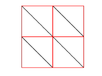
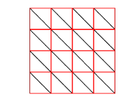
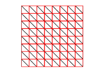
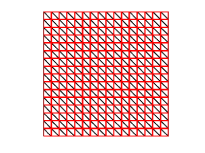
(a) Initial structured grids.

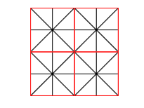
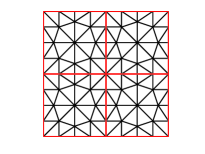
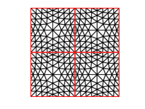
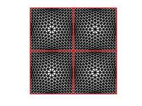
(b) First three refinement levels of unstructured triangular grids on a subdomain partition made of $N=4$ squares.

Figure 1: Top: initial structured grids on subdomains partitions made by $N=4^{\ell}$ squares, $\ell=1,2,3,4$. Bottom: first four refinement levels of unstructured grids on a subdomain partition made of $N=4$ squares.

Throughout the section, we have solved the (preconditioned) linear system of equations by the Preconditioned Conjugate Gradient (PCG) method with a relative tolerance set equal to $10^{-9}$. The condition number of the (preconditioned) Schur complement matrix has been estimated within the PCG iteration by exploiting the analogies between the Lanczos technique and the PCG method (see [36, Sects. 9.3, 10.2], for more details). Finally, we choose the source term in problem (1) as $f(x,y)=1$, and set the penalty parameter $\alpha$ equal to $10$.

We first present some computations that show the behavior of the condition number of the Schur complement matrix ${\mathbf{S}}$, cf. (5).

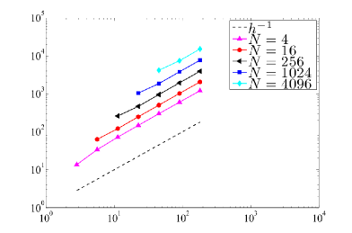
Figure 2: Condition number estimate of the Schur complement matrix ${\mathbf{S}}$ versus $1/h$ on different subdomains partitions made by $N=4^{\ell}$ squares, $\ell=1,2,3,4,5$. Structured (left) and unstructured (right) triangular grids. piecewise linear elements ($p=1$).

In Figure 2 (log-log scale) we report, for different subdomains partitions made by $N=4^{\ell}$ squares, $\ell=1,2,3,4,5$, the condition number estimate of the Schur complement matrix ${\mathbf{S}}$, $\kappa({\mathbf{S}})$, as a function of the mesh-size $1/h$. We clearly observe that $\kappa({\mathbf{S}})$ increases linearly as the mesh size $h$ goes to zero.

Next, we consider the preconditioned linear system of equations

$${\mathbf{P}}^{-1}\widetilde{{\mathbf{S}}}\,\widetilde{{\mathbf{u}}}={\mathbf{P}}^{-1}\widetilde{{\mathbf{g}}},$$

and test the performance of the preconditioners ${\mathbf{P}}$ and ${\mathbf{P}}_{\star}$ (cf. (33) and (34), respectively). Throughout the section, the action of the preconditioner has been computed with a direct solver.

In the first set of experiments, we consider piecewise linear elements ($p=1$), and compute the condition number estimates when varying the number of subdomains and the mesh size. Table 1 shows the condition number estimates increasing the number of subdomains $N$ and the number of elements $n$ of the fine mesh. In Table 1 we also report (between parenthesis) the ratio between the condition number of the preconditioned system and $\left(1+\log(H/h)\right)^{2}$ (between parenthesis). These results have been obtained on a sequence of structured triangular grids as the ones shown in Figure 1(a). Results reported in Table 1 (top) refers to the performance of the preconditioner ${\mathbf{P}}$, whereas the analogous results obtained with the preconditioner ${\mathbf{P}}_{\star}$ are shown in Table 1 (bottom).

	Preconditioner ${\mathbf{P}}$
$N\downarrow\;n\rightarrow\;$	$n=128$	$n=512$	$n=2048$	$n=8192$	$n=32768$
$N=16$	3.11 (0.74)	4.88 (0.65)	7.50 (0.64)	10.84 (0.64)	14.79 (0.64)
$N=64$	-	3.30 (0.79)	5.25 (0.70)	8.00 (0.68)	11.42 (0.67)
$N=256$	-	-	3.35 (0.81)	5.36 (0.72)	8.16 (0.70)
$N=1024$	-	-	-	3.37 (0.81)	5.39 (0.72)
	Preconditioner ${\mathbf{P}}_{\star}$
	$n=128$	$n=512$	$n=2048$	$n=8192$	$n=32768$
$N=16$	2.26 (0.54)	4.04 (0.54)	7.01 (0.60)	11.00 (0.65)	15.83 (0.68)
$N=64$	-	2.42 (0.58)	4.49 (0.60)	7.85 (0.67)	12.28 (0.72)
$N=256$	-	-	2.47 (0.59)	4.60 (0.62)	8.07 (0.69)
$N=1024$	-	-	-	2.48 (0.60)	4.63 (0.62)

Table 1: Preconditioner ${\mathbf{P}}$ (top) and ${\mathbf{P}}_{\star}$ (bottom). Condition number estimates and ratio between the condition number of the preconditioned system and $\left(1+\log(H/h)\right)^{2}$ (between parenthesis). Structured triangular grids, piecewise linear elements ($p=1$).

We have repeated the same set of experiments on the sequence of unstructured triangular grids (cf. Figure 1(b)). The computed results are shown in Figure 2. As before, between parenthesis we report ratio between the condition number of the preconditioned system and $\left(1+\log(H/h)\right)^{2}$. As expected, a logarithmic growth is clearly observed for both preconditioner ${\mathbf{P}}$ and ${\mathbf{P}}_{\star}$.

	Preconditioner ${\mathbf{P}}$
	$n=128$	$n=512$	$n=2048$	$n=8192$	$n=32768$
$N=16$	2.87 (0.69)	4.69 (0.63)	7.35 (0.63)	10.68 (0.63)	14.62 (0.63)
$N=64$	-	3.05 (0.73)	5.01 (0.67)	7.75 (0.66)	11.13 (0.66)
$N=256$	-	-	3.09 (0.74)	5.08 (0.68)	7.89 (0.67)
$N=1024$	-	-	-	3.11 (0.75)	5.11 (0.68)
	Preconditioner ${\mathbf{P}}_{\star}$
	$n=128$	$n=512$	$n=2048$	$n=8192$	$n=32768$
$N=16$	1.84 (0.44)	3.24 (0.43)	5.51 (0.47)	8.44 (0.50)	12.00 (0.52)
$N=64$	-	2.01 (0.48)	3.77 (0.50)	6.35 (0.54)	9.76 (0.58)
$N=256$	-	-	2.04 (0.49)	3.90 (0.52)	6.58 (0.56)
$N=1024$	-	-	-	2.05 (0.49)	3.93 (0.53)

Table 2: Preconditioner ${\mathbf{P}}$ (top) and ${\mathbf{P}}_{\star}$ (bottom). Condition number estimates and ratio between the condition number of the preconditioned system and $\left(1+\log(H/h)\right)^{2}$ (between parenthesis). Unstructured triangular grids, piecewise linear elements ($p=1$).

Next, always with $p=1$, we present some computations that show that the preconditioner ${\mathbf{P}}_{D}$ defined as in (35), i.e., the block-diagonal version of the preconditioner ${\mathbf{P}}_{\star}$, is not optimal (cf. Remark 5.2). More precisely, in Table 3 we report the condition number estimate of the preconditioned system when decreasing $H$ as well as $h$. Table 3 also shows (between parenthesis) the ratio between $\kappa({\mathbf{P}}_{D}\widetilde{{\mathbf{S}}})$ and $Hh^{-1}$. We can clearly observe that on both structured and unstructured mesh configurations, the ratio between $\kappa({\mathbf{P}}_{D}\widetilde{{\mathbf{S}}})$ and $Hh^{-1}$ remains substantially constant as $H$ and $h$ vary, indicating that the preconditioner ${\mathbf{P}}_{D}$ is not optimal.

	Structured triangular grids
	$n=128$	$n=512$	$n=2048$	$n=8192$	$n=32768$
$N=16$	11.51 (4.07)	23.19 (4.10)	47.40 (4.19)	95.21 (4.21)	190.69 (4.21)
$N=64$	-	11.58 (4.09)	23.03 (4.07)	47.16 (4.17)	95.02 (4.20)
$N=256$	-	-	11.55 (4.08)	22.96 (4.06)	47.12 (4.16)
$N=1024$	-	-	-	11.44 (4.04)	22.88 (4.04)
	Unstructured triangular grids
	$n=128$	$n=512$	$n=2048$	$n=8192$	$n=32768$
$N=16$	9.45 (3.34)	18.63 (3.29)	39.13 (3.46)	75.38 (3.33)	148.93 (3.29)
$N=64$	-	8.93 (3.16)	18.30 (3.24)	38.88 (3.44)	78.82 (3.48)
$N=256$	-	-	8.80 (3.11)	17.85 (3.15)	38.59 (3.41)
$N=1024$	-	-	-	8.75 (3.10)	17.64 (3.12)

Table 3: Preconditioner ${\mathbf{P}}_{D}$. Condition number estimates and ratio between $\kappa({\mathbf{P}}_{D}\widetilde{{\mathbf{S}}})$ and $Hh^{-1}$ (between parenthesis). Structured (top) and unstructured (bottom) triangular grids, piecewise linear elements ($p=1$).

Finally, we present some computations obtained with high-order elements. As before, we consider a subdomain partition made of $N=4^{\ell}$ squares, $\ell=1,2,\ldots$, (cf. Figure 1(a) for $\ell=1,2,3$). In this set of experiments, the subdomain partition coincides with the fine grid, i.e., $H=h$ , and on each element we consider the space of polynomials of degree $p=2,3,4,5,6$ in each coordinate direction.

Table 4 shows the condition number estimate of the non-preconditioned Schur complement matrix and the CG iteration counts.

$N=n$	$p=2$	$p=3$	$p=4$	$p=5$	$p=6$
$4$	5.1e+1 ( 5)	2.7e+2 ( 8)	6.2e+2 (13)	1.4e+3 (18)	3.4e+3 (28)
$16$	3.2e+2 (22)	8.4e+2 (42)	2.0e+3 (69)	4.6e+3 (101)	1.1e+4 (153)
$64$	1.2e+3 (90)	3.2e+3 (150)	7.6e+3 (231)	1.8e+4 (312)	4.3e+4 (446)
$256$	4.7e+3 (195)	1.3e+4 (294)	3.0e+4 (462)	7.0e+4 (634)	1.7e+5 (886)

Table 4: Condition number estimates $\kappa({\mathbf{S}})$ and CG iteration counts (between parenthesis). Cartesian grids.

We have run the same set of experiments employing the preconditioners ${\mathbf{P}}$ and ${\mathbf{P}}_{\star}$, and the results are reported in Table 5 . We clearly observe that, as predicted, for a fixed mesh configuration the condition number of the preconditioned system grows logarithmically as the polynomial approximation degree increases. Comparing these results with the analogous ones reported in Table 4, it can be inferred that both the preconditioners ${\mathbf{P}}$ and ${\mathbf{P}}_{\star}$ are efficient in reducing the condition number of the Schur complement matrix.

	Preconditioner ${\mathbf{P}}$
$N=n$	$p=2$	$p=3$	$p=4$	$p=5$	$p=6$
$N=4$	7.14 (1.25)	9.04 (0.88)	12.06 (0.85)	14.15 (0.79)	16.48 (0.78)
$N=16$	9.24 (1.62)	9.93 (0.97)	15.25 (1.07)	15.99 (0.90)	20.25 (0.96)
$N=64$	10.03 (1.76)	10.14 (0.99)	16.34 (1.15)	16.57 (0.93)	21.53 (1.02)
$N=256$	10.24 (1.80)	10.19 (1.00)	16.61 (1.17)	16.71 (0.94)	21.84 (1.04)
	Preconditioner ${\mathbf{P}}_{\star}$
$N=n$	$p=2$	$p=3$	$p=4$	$p=5$	$p=6$
$N=4$	1.88 (0.33)	2.56 (0.25)	3.75 (0.26)	4.64 (0.26)	5.70 (0.27)
$N=16$	4.60 (0.81)	5.23 (0.51)	8.71 (0.61)	9.38 (0.53)	12.25 (0.58)
$N=64$	6.18 (1.09)	6.03 (0.59)	10.35 (0.73)	10.79 (0.61)	14.33 (0.68)
$N=256$	6.55 (1.15)	6.25 (0.61)	10.83 (0.76)	11.20 (0.63)	14.94 (0.71)

Table 5: Preconditioner ${\mathbf{P}}$ (top), ${\mathbf{P}}_{\star}$ (bottom). Condition number estimates and ratio between the condition number of the preconditioned system and $\left(1+\log(p^{2})\right)^{2}$ (between parenthesis). Cartesian grids.

Appendix A Appendix

In this section, we report the proofs of Lemma 3.1 and Lemma 3.2.

In the following, for $E\subset\Omega_{\ell}$ subdomain edge we will make explicit use of the space $H^{s}_{0}(E)$, $0<s<1/2$, which is defined as the subspace of those functions $\eta$ of $H^{s}(E)$ such that the function $\bar{\eta}\in L^{2}(\partial{\Omega_{\ell}})$ defined as $\bar{\eta}=\eta$ on $E$ and $\bar{\eta}=0$ on $\partial{\Omega_{\ell}}\setminus E$ belongs to $H^{s}(\partial{\Omega_{\ell}})$. The space $H^{s}_{0}(E)$ is endowed with the norms

$$\|\eta\|_{H^{s}_{0}(E)}=\|\bar{\eta}\|_{H^{s}(\partial{\Omega_{\ell}})}.$$

We recall that for $s<1/2$ the spaces $H^{s}(E)$ and $H^{s}_{0}(E)$ coincide as sets and have equivalent norms. However, the constant in the norm equivalence goes to infinity as $s$ tends to $1/2$. In particular on the reference segment $\widehat{E}=(0,1)$, for all $\varphi\in H^{s}(\widehat{E})$ and for all $\beta\in{\mathbb{R}}$, the following bound can be shown (see [15])

$$|\varphi|_{H^{s}_{0}(\widehat{E})}\lesssim\frac{1}{1/2-s}\|\varphi-\beta\|_{H^{s}(\widehat{E})}+\frac{1}{\sqrt{1/2-s}}|\beta|,$$

which, provided $\varphi\in H^{1/2}(\widehat{E})$, implies the bound

$$|\varphi|_{H^{s}_{0}(\widehat{E})}\lesssim\frac{1}{1/2-s}\|\varphi-\beta\|_{H^{1/2}(\widehat{E})}+\frac{1}{\sqrt{1/2-s}}|\beta|.$$ (36)

Prior to give the proofs of Lemmas 3.1 and 3.2, we start by observing that the following result, that corresponds to the $hp$-version of [15, Lemma 3.1], holds.

Lemma A.1.

Let $E=(a,b)$ be a subdomain edge of ${\Omega_{\ell}}$. Then, for all $\eta\in\Phi_{\ell}(E)$, the following bounds hold:

• $$(\eta(a)-\eta(b))^{2}\lesssim\left(1+\log{\left(\frac{H_{\ell}\,p_{\ell}^{2}}{h_{\ell}}\right)}\right)|\eta|^{2}_{H^{1/2}(E)}.$$ (37)

• If $\eta(x)=0$ at some $x\in E$ it holds

  $$\|\eta\|^{2}_{L^{\infty}(E)}\lesssim\left(1+\log{\left(\frac{H_{\ell}\,p_{\ell}^{2}}{h_{\ell}}\right)}\right)|\eta|^{2}_{H^{1/2}(E)}.$$ (38)

• if $\eta\in\Phi^{0}_{\ell}(E)$, we have

  $$\|\eta\|_{H^{1/2}_{00}(E)}^{2}\lesssim\left(1+\log{\left(\frac{H_{\ell}\,p_{\ell}^{2}}{h_{\ell}}\right)}\right)|\eta|_{H^{1/2}(\partial{\Omega_{\ell}})}^{2}.$$ (39)

Proof.

We first show (ii). Notice that since $E$ is an arbitrary subdomain edge, $E\subset\partial{\Omega_{\ell}}$, and so $|E|\simeq H_{\ell}$. We claim that for any $\varphi\in H^{1/2+\varepsilon}(E)$ the following inequality holds:

$$\|\varphi\|^{2}_{L^{\infty}(E)}\lesssim H^{-1}_{\ell}\|\varphi\|_{L^{2}(E)}^{2}+\frac{H^{2\varepsilon}_{\ell}}{\varepsilon}|\varphi|^{2}_{H^{1/2+\varepsilon}(E)}.$$ (40)

To show (40) one needs to trace the constants in the Sobolev imbedding between $H^{1/2+\varepsilon}(E)$ and $L^{\infty}(E)$. Let $\widehat{E}=]0,1[$ be the reference unit segment. Then, for any $\hat{\varphi}\in H^{1/2+\varepsilon}(\widehat{E})$, the continuity constant of the injection $H^{1/2+\varepsilon}(\widehat{E})\subset L^{\infty}(\widehat{E})$ depends on $\varepsilon$ as follows (see [15, Appendix], for details)

$$\|\hat{\varphi}\|^{2}_{L^{\infty}(\widehat{E})}\lesssim\|\hat{\varphi}\|_{L^{2}(\widehat{E})}^{2}+\frac{1}{\varepsilon}|\hat{\varphi}|^{2}_{H^{1/2+\varepsilon}(\widehat{E})}.$$

A scaling argument using $|E|\simeq H_{\ell}$ leads to (40).

Let now $\eta\in\Phi_{h}$ and $\beta\in\mathbb{R}$ an arbitrary constant. Using the inverse inequality (10), we have

$$\frac{H_{\ell}^{2\varepsilon}}{\varepsilon}|\eta-\beta|^{2}_{H^{1/2+\varepsilon}(E)} =\frac{H_{\ell}^{2\varepsilon}}{\varepsilon}|\eta|^{2}_{H^{1/2+\varepsilon}(E)}\lesssim\frac{H_{\ell}^{2\varepsilon}\,p_{\ell}^{4\varepsilon}h_{\ell}^{-2\varepsilon}}{\varepsilon}|\eta|^{2}_{H^{1/2}(E)}$$ (41)

$$\lesssim\log{\left(\frac{H_{\ell}\,p_{\ell}^{2}}{h_{\ell}}\right)}|\eta|^{2}_{H^{1/2}(E)}\;,$$

where in the last step we have taken $\varepsilon=1/\log(H_{\ell}p_{\ell}^{2}/h_{\ell})$ and used the fact that $s^{1/\log(s)}=e$. Applying now inequality (40) to $\varphi=\eta-\beta$ together with the above estimate (41) yields:

$$\|\eta-\beta\|_{L^{\infty}(E)}^{2}\lesssim H_{\ell}^{-1}\|\eta-\beta\|^{2}_{L^{2}(E)}+\log\left(\frac{H_{\ell}p_{\ell}^{2}}{h_{\ell}}\right)|\eta|_{H^{1/2}(E)}^{2}.$$ (42)

Following [18], let $\beta$ be the average over $E$ of $\eta$ (or the $L^{2}$- projection onto the space $\mathbb{P}^{0}(E))$ of constants functions over $E$. Poincarè-Friederichs inequality (or standard approximation results) give

$$H_{\ell}^{-1/2}\|\eta-\beta\|_{L^{2}(E)}\lesssim|\eta|_{H^{1/2}(E)}$$ (43)

which yields

$$\|\eta-\beta\|^{2}_{L^{\infty}(E)}\lesssim\left(1+\log\left(\frac{H_{\ell}p_{\ell}^{2}}{h_{\ell}}\right)\right)|\eta|^{2}_{H^{1/2}(E)}.$$ (44)

The proof of (38) is concluded by noticing that if $\eta(x)=0$ for some $x\in\bar{E}$ then it follows

$$|\beta|\lesssim\|\eta-\beta\|_{L^{\infty}(E)}$$ (45)

which yields (38) using triangular inequality.

The proof of (37) follows by applying the estimate (38) to the function $\eta-\eta(a)$, which by hypothesis vanishes at $a\in\bar{E}$.

To show (iii), we first notice that for $\eta_{o}\in\Phi^{o}_{\ell}(E)$, we can always construct an extension $\widetilde{\eta}_{o}$ such that

$$\widetilde{\eta}_{o}=\eta_{o}\;\textrm{ on $E$} \quad\widetilde{\eta}_{o}=0\;\textrm{ on $\partial{\Omega_{\ell}}\setminus E$}\;.$$

Using now the inverse inequality (11), we obtain the following bounds

$$\|\eta_{o}\|_{H^{1/2}_{00}(E)}\lesssim|\widetilde{\eta}_{o}|_{H^{1/2}(\partial{\Omega_{\ell}})}\lesssim p_{\ell}^{2\varepsilon}h_{\ell}^{-\varepsilon}|\tilde{\eta}_{o}|_{H^{1/2-\varepsilon}(\partial{\Omega_{\ell}})}\lesssim p_{\ell}^{2\varepsilon}h_{\ell}^{-\varepsilon}|\eta_{o}|_{H^{1/2-\varepsilon}_{0}(E)},$$ (46)

where the second inequality follows from the boundedness from $H^{1/2}_{00}(E)$ to $H^{1/2}(\partial{\Omega_{\ell}})$ of the extension by $0$.

To estimate now the $H^{1/2-\varepsilon}_{0}(E)$ seminorm of $\eta_{o}$ we observe that (36) rescales as

$$|\varphi|_{H^{1/2-\varepsilon}_{0}(E)}\lesssim\frac{H_{\ell}^{\varepsilon}}{\varepsilon}\left(H_{\ell}^{-1/2}\|\varphi-\beta\|_{L^{2}(E)}+|\varphi-\beta|_{H^{1/2}(E)}\right)+\frac{H_{\ell}^{\varepsilon}}{\sqrt{\varepsilon}}|\beta|.$$

Taking now $\varphi=\eta_{o}$ and choosing $\beta$ as its average on $E$, the first term on the right hand side above is bounded by means of Poincaré-Friederichs inequality, and the second by means of estimate (45), which holds since $\eta_{o}(a)=0$. Hence, we get

$$\|\eta_{o}\|_{H^{1/2}_{00}(E)}\lesssim\frac{H_{\ell}^{\varepsilon}p_{\ell}^{2\varepsilon}h_{\ell}^{-\varepsilon}}{\varepsilon}|\eta_{o}|_{H^{1/2}(E)}+\frac{H_{\ell}^{\varepsilon}p_{\ell}^{2\varepsilon}h_{\ell}^{-\varepsilon}}{\sqrt{\varepsilon}}\|\eta_{o}-\beta\|_{L^{\infty}(E)}.$$

Arguing as before and taking $\varepsilon=1/\log(H_{\ell}p_{\ell}^{2}/h_{\ell})$, and using bound (44) we obtain

$$\|\eta_{o}\|_{H^{1/2}_{00}(E)}\lesssim\left(1+\log\frac{H_{\ell}\,p_{\ell}^{2}}{h_{\ell}}\right)|\eta_{o}|_{H^{1/2}(E)}.$$

Finally, since $\sum_{E\subset\partial{\Omega_{\ell}}}|\cdot|_{H^{1/2}(E)}^{2}\lesssim|\cdot|_{H^{1/2}(\partial{\Omega_{\ell}})}^{2},$ by squaring and taking the sum over $E\subset\partial{\Omega_{\ell}}$, we obtain (39). ∎

We are now able to prove Lemma 3.1 and Lemma 3.2.

Proof of Lemma 3.1..

A direct computation using the linearity of $\chi$ shows that, if $a_{i},b_{i}$ are the vertices of the $i$-th subdomain edge $E^{i}$ of ${\Omega_{\ell}}$, we have

$$|\chi^{\ell}|_{H^{1/2}(\partial{\Omega_{\ell}})}^{2}\lesssim\sum_{i=1}^{N^{\ell}_{E}}(\eta^{\ell}(a_{i})-\eta^{\ell}(b_{i}))^{2}$$

with $N^{\ell}_{E}$($=3$ or $4$) denoting the number of subdomain edges of ${\Omega_{\ell}}$. Now, using  (37) and assembling all the contributions we easily conclude that the thesis holds.

∎

Proof of Lemma 3.2.

Let $\zeta_{0}\in\Phi_{h}^{\ell}$ be the unique element of $\Phi_{h}^{\ell}$ satisfying $\zeta_{0}(a)=0$ for all vertices $a$ of ${\Omega_{\ell}}$ and $(\zeta_{0},\tau)_{H^{1/2}(\partial{\Omega_{\ell}})}=(\zeta_{L},\tau)_{H^{1/2}(\partial{\Omega_{\ell}})}$ for all $\tau\in\Phi_{h}^{\ell}$ with $\tau(a)=0$ for all vertices $a$ of ${\Omega_{\ell}}$. It is not difficult to see that $|\cdot|_{H^{1/2}(\partial{\Omega_{\ell}})}$ is a norm on the subspace of functions in $\Phi_{h}^{\ell}$ vanishing at the vertices of ${\Omega_{\ell}}$ and then, by standard arguments we get that $\zeta_{0}$ is well defined and $|\zeta_{0}|_{H^{1/2}(\partial{\Omega_{\ell}})}\lesssim|\zeta_{L}|_{H^{1/2}(\partial{\Omega_{\ell}})}$. Now we can write:

$$\sum_{i=1}^{N^{\ell}_{E}}\|\xi\|^{2}_{H^{1/2}_{00}({E_{\ell}^{i}})}\lesssim\sum_{i=1}^{N^{\ell}_{E}}\|\xi+\zeta_{0}\|^{2}_{H^{1/2}_{00}({E_{\ell}^{i}})}+\sum_{i=1}^{N^{\ell}_{E}}\|\zeta_{0}\|^{2}_{H^{1/2}_{00}({E_{\ell}^{i}})},$$ (47)

with $N^{\ell}_{E}$ number of subdomain edges of ${\Omega_{\ell}}$. The first sum on the right hand side of (47) can be bound by using the previous lemma as

$$\sum_{i=1}^{N^{\ell}_{E}}\|\xi+\zeta_{0}\|^{2}_{H^{1/2}_{00}({E_{\ell}^{i}})} \lesssim\left(1+\log\left(\frac{H_{\ell}\,p_{\ell}^{2}}{h_{\ell}}\right)\right)^{2}|\xi+\zeta_{0}|^{2}_{H^{1/2}(\partial{\Omega_{\ell}})}$$

$$\lesssim\left(1+\log\left(\frac{H_{\ell}\,p_{\ell}^{2}}{h_{\ell}}\right)\right)^{2}|\xi+\zeta_{L}|^{2}_{H^{1/2}(\partial{\Omega_{\ell}})},$$

where on one hand we used Poincaré inequality to bound the $H^{1/2}$ norm of $\xi+\zeta_{0}$ (which vanishes at the vertices of ${\Omega_{\ell}}$) by the corresponding seminorm, while the last inequality follows by observing that, by the definition of $\zeta_{0}$, $\xi+\zeta_{0}\in\Phi_{h}^{\ell}$ vanishes at the vertices of ${\Omega_{\ell}}$ and satisfies $(\zeta_{L}-\zeta_{0},\xi+\zeta_{0})_{H^{1/2}(\partial{\Omega_{\ell}})}=0$. Hence, we have

$$|\xi+\zeta_{L}|^{2}_{H^{1/2}(\partial{\Omega_{\ell}})}=|\xi+\zeta_{0}|^{2}_{H^{1/2}(\partial{\Omega_{\ell}})}+|\zeta_{L}-\zeta_{0}|^{2}_{H^{1/2}(\partial{\Omega_{\ell}})}\geq|\xi+\zeta_{0}|^{2}_{H^{1/2}(\partial{\Omega_{\ell}})}.$$

Let us now bound the second sum on the right hand side of (47): we first observe that

$$\|\zeta_{0}\|^{2}_{H^{1/2}_{00}({E_{\ell}^{i}})}=|\zeta_{0}|^{2}_{H^{1/2}({E_{\ell}^{i}})}+I_{1}(\zeta_{0})+I_{2}(\zeta_{0}),$$

having set

$$I_{1}(\zeta_{0})=\int_{a_{i}}^{b_{i}}\frac{|\zeta_{0}(x)|^{2}}{|x-{a_{i}}|}\,\textrm{dx}, I_{2}(\zeta_{0})=\int_{a_{i}}^{b_{i}}\frac{|\zeta_{0}(x)|^{2}}{|x-{b_{i}}|}\,\textrm{dx},$$

with ${a_{i}}$ and ${b_{i}}$ the two vertices of the subdomain edge ${E_{\ell}^{i}}$. Now we can write

$$\sum_{i=1}^{N^{\ell}_{E}}|\zeta_{0}|^{2}_{H^{1/2}({E_{\ell}^{i}})} \lesssim|\zeta_{0}|^{2}_{H^{1/2}(\partial{\Omega_{\ell}})}\lesssim|\zeta_{L}|^{2}_{H^{1/2}(\partial{\Omega_{\ell}})}\lesssim\sum_{i=1}^{N^{\ell}_{E}}(\zeta_{L}({a_{i}})-\zeta_{L}({b_{i}}))^{2}$$

$$\lesssim\left(1+\log\left(\frac{H_{\ell}\,p_{\ell}^{2}}{h_{\ell}}\right)\right)|\xi+\zeta_{L}|^{2}_{H^{1/2}(\partial{\Omega_{\ell}})},$$

where the inequality $|\zeta_{L}|^{2}_{H^{1/2}(\partial{\Omega_{\ell}})}\lesssim\sum_{i=1}^{N^{\ell}_{E}}(\zeta_{L}({a_{i}})-\zeta_{L}({b_{i}}))^{2}$ is proven in [18] by direct computation, and the last inequality follows by applying the bound of Lemma A.1-(ii) to the function $(\xi+\zeta_{L})(x)-(\xi+\zeta_{L})({b_{i}})$.

Let us now bound $I_{1}$. For notational simplicity let us identify ${a_{i}}=0$ and ${b_{i}}=H$. Adding and subtracting $\zeta_{L}(x)+\zeta_{L}(0)$ and using the Cauchy-Schwarz inequality, we have

$$I_{1}(\zeta_{0})=\int_{0}^{H}\frac{|\zeta_{0}(x)|^{2}}{|x|}\,\textrm{dx}\lesssim\int_{0}^{H}\frac{|\zeta_{0}(x)-\zeta_{L}(x)+\zeta_{L}(0)|^{2}}{|x|}\,\textrm{dx}+\int_{0}^{H}\frac{|\zeta_{L}(x)-\zeta_{L}(0)|^{2}}{|x|}\,\textrm{dx}.$$ (48)

Let us bound the first integral on the right hand side of (48). Setting $\zeta_{\perp}=\zeta_{0}-\zeta_{L}$, we have

$$\int_{0}^{H}\frac{|\zeta_{\perp}(x)-\zeta_{\perp}(0)|^{2}}{|x|}\,\textrm{dx}=\int_{0}^{h}\frac{|\zeta_{\perp}(x)-\zeta_{\perp}(0)|^{2}}{|x|}\,\textrm{dx}+\int_{h}^{H}\frac{|\zeta_{\perp}(x)-\zeta_{\perp}(0)|^{2}}{|x|}\,\textrm{dx}.$$

The first term can be bounded by

$$\int_{0}^{h}\frac{|\zeta_{\perp}(x)-\zeta_{\perp}(0)|^{2}}{|x|}\,\textrm{dx}=\int_{0}^{h}\frac{|\int_{0}^{x}(\zeta_{\perp})_{x}(\tau)\,d\tau|^{2}}{|x|}\,\textrm{dx}\lesssim h|\zeta_{\perp}|^{2}_{H^{1}({E_{\ell}^{i}})}\lesssim|\zeta_{\perp}|^{2}_{H^{1/2}({E_{\ell}^{i}})},$$

while we bound the second term by

$$\int_{h}^{H}\frac{|\zeta_{\perp}(x)-\zeta_{\perp}(0)|^{2}}{|x|}\,\textrm{dx}\lesssim \|\zeta_{\perp}-\zeta_{\perp}(0)\|^{2}_{L^{\infty}({E_{\ell}^{i}})}\log\left(\frac{H_{\ell}\,p_{\ell}^{2}}{h_{\ell}}\right)$$

$$\lesssim \left(\log\left(\frac{H_{\ell}\,p_{\ell}^{2}}{h_{\ell}}\right)\right)^{2}|\zeta_{\perp}|^{2}_{H^{1/2}({E_{\ell}^{i}})}.$$

Next, we estimate the second integral on the right hand side of (48). By direct calculation and using the linearity of $\zeta_{L}$, we have

$$\int_{0}^{H}\frac{|\zeta_{L}(x)-\zeta_{L}(0)|^{2}}{|x|}\,\textrm{dx}\lesssim(\zeta_{L}(B_{\ell})-\zeta_{L}(A_{\ell}))^{2}\lesssim\log\left(\frac{H_{\ell}\,p_{\ell}}{h_{\ell}}\right)\,|\zeta_{L}+\xi|^{2}_{H^{1/2}({E_{\ell}^{i}})}.$$

Hence, we conclude that

$$I_{1}(\zeta_{0})\lesssim\left(1+\log\left(\frac{H_{\ell}\,p_{\ell}^{2}}{h_{\ell}}\right)\right)^{2}|\zeta_{0}-\zeta_{L}|^{2}_{H^{1/2}({E_{\ell}^{i}})}+\log\left(\frac{H_{\ell}\,p_{\ell}^{2}}{h_{\ell}}\right)\,|\zeta_{L}+\xi|^{2}_{H^{1/2}({E_{\ell}^{i}})}.$$

The term $I_{2}$ can be bounded by the same argument. Collecting all the previous estimates the thesis follows. ∎

References

- [1] Yves Achdou, Yvon Maday, and Olof B. Widlund. Iterative substructuring preconditioners for mortar element methods in two dimensions. SIAM J. Numer. Anal., 36(2):551–580 (electronic), 1999.
- [2] Mark Ainsworth. A preconditioner based on domain decomposition for - finite-element approximation on quasi-uniform meshes. SIAM J. Numer. Anal., 33(4):1358–1376, 1996.
- [3] Paola F. Antonietti and Blanca Ayuso. Schwarz domain decomposition preconditioners for discontinuous Galerkin approximations of elliptic problems: non-overlapping case. M2AN Math. Model. Numer. Anal., 41(1):21–54, 2007.
- [4] Paola F. Antonietti and Blanca Ayuso. Multiplicative Schwarz methods for discontinuous Galerkin approximations of elliptic problems. M2AN Math. Model. Numer. Anal., 42(3):443–469, 2008.
- [5] Paola F. Antonietti and Blanca Ayuso. Two-level Schwarz preconditioners for super penalty discontinuous Galerkin methods. Commun. Comput. Phys., 5(2-4):398–412, 2009.
- [6] Paola F. Antonietti and Paul Houston. A class of domain decomposition preconditioners for -discontinuous Galerkin finite element methods. J. Sci. Comput., 46(1):124–149, 2011.
- [7] Douglas N. Arnold, Franco Brezzi, Bernardo Cockburn, and L. Donatella Marini. Unified analysis of discontinuous Galerkin methods for elliptic problems. SIAM J. Numer. Anal., 39(5):1749–1779, 2001/02.
- [8] Douglas N. Arnold, Franco Brezzi, Richard S. Falk, and L. Donatella Marini. Locking-free Reissner-Mindlin elements without reduced integration. Comput. Methods Appl. Mech. Engrg., 196(37-40):3660–3671, 2007.
- [9] Douglas N. Arnold, Franco Brezzi, and L. Donatella Marini. A family of discontinuous Galerkin finite elements for the Reissner-Mindlin plate. J. Sci. Comput., 22/23:25–45, 2005.
- [10] B. Ayuso de Dios, M. Holst, Y. Zhu, and L. Zikatanov. Multilevel preconditioners for discontinuous Galerkin approximations of elliptic problems with jump coefficients. Math. Comp., to appear.
- [11] Blanca Ayuso de Dios, Ivan Georgiev, Johannes Kraus, and Ludmil Zikatanov. Subspace correction methods for discontinuous Galerkin methods discretizations for linear elasticity equations. submitted, 2011.
- [12] Blanca Ayuso de Dios and Ludmil Zikatanov. Uniformly convergent iterative methods for discontinuous Galerkin discretizations. J. Sci. Comput., 40(1-3):4–36, 2009.
- [13] Andrew T. Barker, Susanne C. Brenner, Park Eun-Hee, and Li-Yeng Sung. Two-level additive Schwarz preconditioners for a weakly over-penalized symmetric interior penalty method. J. Sci. Comp., 47:27–49, 2011.
- [14] Roland Becker, Peter Hansbo, and Rolf Stenberg. A finite element method for domain decomposition with non-matching grids. M2AN Math. Model. Numer. Anal., 37(2):209–225, 2003.
- [15] Silvia Bertoluzza. Substructuring preconditioners for the three fields domain decomposition method. Math. Comp., 73(246):659–689 (electronic), 2004.
- [16] Silvia Bertoluzza and Micol Pennacchio. Analysis of substructuring preconditioners for mortar methods in an abstract framework. Appl. Math. Lett., 20(2):131–137, 2007.
- [17] Petter E. Bjørstad and Olof B. Widlund. Iterative methods for the solution of elliptic problems on regions partitioned into substructures. SIAM J. Numer. Anal., 23(6):1093–1120, 1986.
- [18] James H. Bramble, Joseph E. Pasciak, and Alfred H. Schatz. The construction of preconditioners for elliptic problems by substructuring. I. Math. Comp., 47(175):103–134, 1986.
- [19] James H. Bramble, Joseph E. Pasciak, and Alfred H. Schatz. The construction of preconditioners for elliptic problems by substructuring. IV. Math. Comp., 53(187):1–24, 1989.
- [20] Susanne C. Brenner and Kening Wang. Two-level additive Schwarz preconditioners for interior penalty methods. Numer. Math., 102(2):231–255, 2005.
- [21] Susanne C. Brenner and Jie Zhao. Convergence of multigrid algorithms for interior penalty methods. Appl. Numer. Anal. Comput. Math., 2(1):3–18, 2005.
- [22] Kolja Brix, Martin Campos Pinto, and Wolfgang Dahmen. A multilevel preconditioner for the interior penalty discontinuous Galerkin method. SIAM J. Numer. Anal., 46(5):2742–2768, 2008.
- [23] Claudio Canuto, Luca F. Pavarino, and Alexandre B. Pieri. BDDC preconditioners for Continuous and Discontinuous Galerkin methods using spectral/hp elements with variable local polynomial degree. Technical report, 2012. (submitted).
- [24] Bernardo Cockburn, Jayadeep Gopalakrishnan, and Raytcho Lazarov. Unified hybridization of discontinuous Galerkin, mixed, and continuous Galerkin methods for second order elliptic problems. SIAM J. Numer. Anal., 47(2):1319–1365, 2009.
- [25] Bernardo Cockburn, Guido Kanschat, and Dominik Schötzau. A note on discontinuous Galerkin divergence-free solutions of the Navier-Stokes equations. J. Sci. Comput., 31(1-2):61–73, 2007.
- [26] James W. Demmel. Applied Numerical Linear Algebra. SIAM, 1997.
- [27] Veselin A. Dobrev, Raytcho D. Lazarov, Panayot S. Vassilevski, and Ludmil T. Zikatanov. Two-level preconditioning of discontinuous Galerkin approximations of second-order elliptic equations. Numer. Linear Algebra Appl., 13(9):753–770, 2006.
- [28] Maksymilian Dryja. A capacitance matrix method for Dirichlet problem on polygon region. Numer. Math., 39:51–64, 1982.
- [29] Maksymilian Dryja, Juan Galvis, and Marcus Sarkis. BDDC methods for discontinuous Galerkin discretization of elliptic problems. J. Complexity, 23(4-6):715–739, 2007.
- [30] Maksymilian Dryja, Juan Galvis, and Marcus Sarkis. Neumann-Neumann methods for a DG discretization of elliptic problems with discontinuous coefficients on geometrically nonconforming substructures. Numer. Methods Partial Differential Equations, 28(4):1194–1226, 2012.
- [31] Maksymilian Dryja and Marcus Sarkis. FETI-DP method for DG discretization of elliptic problems with discontinuous coefficients. Technical report, Instituto de Matematica Pura e Aplicada, Brazil, 2010. submitted.
- [32] Maksymilian Dryja, Barry F. Smith, and Olof B. Widlund. Schwarz analysis of iterative substructuring algorithms for elliptic problems in three dimensions. SIAM J. Numer. Anal., 31(6):1662–1694, 1994.
- [33] Eduardo Gomes Dutra do Carmo and André Vinicius Celani Duarte. A discontinuous finite element-based domain decomposition method. Comput. Methods Appl. Mech. Engrg., 190(8-10):825–843, 2000.
- [34] Herbert Egger and Joachim Schöberl. A hybrid mixed discontinuous Galerkin finite-element method for convection-diffusion problems. IMA J. Numer. Anal., 30(4):1206–1234, 2010.
- [35] Xiaobing Feng and Ohannes A. Karakashian. Two-level additive Schwarz methods for a discontinuous Galerkin approximation of second order elliptic problems. SIAM J. Numer. Anal., 39(4):1343–1365 (electronic), 2001.
- [36] Gene H. Golub and Charles F. Van Loan. Matrix computations. Johns Hopkins Studies in the Mathematical Sciences. Johns Hopkins University Press, Baltimore, MD, third edition, 1996.
- [37] J. Gopalakrishnan and G. Kanschat. A multilevel discontinuous Galerkin method. Numer. Math., 95(3):527–550, 2003.
- [38] Peter Hansbo and Mats G. Larson. Discontinuous Galerkin methods for incompressible and nearly incompressible elasticity by Nitsche’s method. Comput. Methods Appl. Mech. Engrg., 191(17-18):1895–1908, 2002.
- [39] Mika Juntunen and Rolf Stenberg. Nitsche’s method for general boundary conditions. Math. Comp., 78(267):1353–1374, 2009.
- [40] G. Kanschat and B. Rivière. A strongly conservative finite element method for the coupling of Stokes and Darcy flow. J. Comput. Phys., 229(17):5933–5943, 2010.
- [41] Guido Kanschat. Preconditioning methods for local discontinuous Galerkin discretizations. SIAM J. Sci. Comput., 25(3):815–831, 2003.
- [42] Jan Mandel. Iterative solvers by substructuring for the -version finite element method. Comput. Methods Appl. Mech. Engrg., 80(1-3):117–128, 1990. Spectral and high order methods for partial differential equations (Como, 1989).
- [43] J. Nitsche. Über ein Variationsprinzip zur Lösung von Dirichlet-Problemen bei Verwendung von Teilräumen, die keinen Randbedingungen unterworfen sind. Abh. Math. Sem. Univ. Hamburg, 36:9–15, 1971. Collection of articles dedicated to Lothar Collatz on his sixtieth birthday.
- [44] Luca Pavarino. Domain Decomposition Algorithms for the p-version Finite Element Method for Elliptic Problem. PhD thesis, Courant Institute of Mathematical Sciences, New York University, New York, NY, 1992.
- [45] Micol Pennacchio. Substructuring preconditioners for parabolic problems by the mortar method. Int. J. Numer. Anal. Model., 5(4):527–542, 2008.
- [46] Micol Pennacchio and Valeria Simoncini. Substructuring preconditioners for mortar discretization of a degenerate evolution problem. J. Sci. Comput., 36(3):391–419, 2008.
- [47] Eun-Hee S.C. Brenner and Li yeng Sung. A bddc preconditioner for a symmetric interior penalty galerkin method. Technical report. in preparation.
- [48] Joachim Schöberl and Christoph Lehrenfeld. Domain decomposition preconditioning for high order hybrid discontinuous Galerkin methods on tetrahedral meshes. In Advanced finite element methods and applications, volume 66 of Lect. Notes Appl. Comput. Mech., pages 27–56. Springer, Heidelberg, 2013.
- [49] Ch. Schwab. - and -finite element methods. Numerical Mathematics and Scientific Computation. The Clarendon Press Oxford University Press, New York, 1998. Theory and applications in solid and fluid mechanics.
- [50] Rolf Stenberg. Mortaring by a method of J. A. Nitsche. In Computational mechanics (Buenos Aires, 1998), pages CD–ROM file. Centro Internac. Métodos Numér. Ing., Barcelona, 1998.
- [51] Andrea Toselli and Olof Widlund. Domain decomposition methods—algorithms and theory, volume 34 of Springer Series in Computational Mathematics. Springer-Verlag, Berlin, 2005.
- [52] Jinchao Xu and Jun Zou. Some nonoverlapping domain decomposition methods. SIAM Rev., 40(4):857–914, 1998.