Electronic properties of closed cage nanometer-size spherical graphitic particles

Abstract

We investigate the localization of charged particles by the image potential of spherical shells, such as fullerene buckyballs. These spherical image states exist within surface potentials formed by the competition between the attractive image potential and the repulsive centripetal force arising from the angular motion. The image potential has a power law rather than a logarithmic behavior for a nanotube, leading to fundamental differences in the forms for the effective potential for the two geometries. The sphere has localized stable states close to its surface. At low temperatures, this results in long lifetimes for the image states. We predict the possibility of creating image states with binding energies of a few meV around metallic/non-metallic spherical shells by photoionization. Applications and related phenomena are discussed.

The experimental and theoretical study of carbon is currently one of the most prevailing research areas in condensed matter physics. Forms of carbon include several allotropes such as graphene, graphite as well as the fullerenes, which cover any molecule composed entirely of carbon, in the form of a hollow sphere, ellipsoid or tube. Like graphite, fullerenes are composed of stacked graphene sheets of linked hexagonal rings. For these, the carbon atoms form strong covalent bonds through hybridized sp² atomic orbitals between three nearest neighbors in a planar or nearly planar configuration.

Mass spectrometry experiments showed strong peaks corresponding to molecules with the exact mass of sixty carbon atoms and other carbon clusters such as C₇₀, C₇₆, and up to C₉₄ 1 ; 1b . Spherical fullerenes, well known as “buckyballs” (C₆₀), were prepared in 1985 by Kroto, et al. 2 The structure was also identified about five years earlier by Iijima, 3 from an electron microscope image, where it formed the core of a multi-shell fullerene or “bucky onion.” Since then, fullerenes have been found to exist naturally 4 . More recently, fullerenes have been detected in outer space 5 . As a matter of fact, the discovery of fullerenes greatly expanded the number of known carbon allotropes, which until recently were limited to graphite, diamond, and amorphous carbon such as soot and charcoal. Both buckyballs and carbon nanotubes, also referred to as buckytubes have been the focus of intense investigation, for their unique chemistry as well as their technological applications in materials science, electronics, and nanotechnology 6 .

Recently, the image states of metallic carbon nanotubes 7 and double-wall non-metallic nanotubes 8 ; 8b were investigated Experimental work 8c includes photoionization 8c+ and time-resolved photoimaging of image-potential states in carbon nanotubes 8cc+ . There has been general interest 8c++ in these structures because of electronic control on the nanoscale using image states. This has led to wide-ranging potential applications including field ionization of cold atoms near carbon nanotubes, 8d and chemisorption of fluorine atoms on the surface of carbon nanotubes 8e . Here, we calculate the nature of the image-potential states in a spherical electron gas (SEG) confined to the surface of a buckyball in a similar fashion as in the case of a nanotube. For the semi-infinite metal/vacuum interface, 9 related image-potential states have been given a considerable amount of theoretical attention over the years. Additionally, these states have been observed for pyrolytic graphite 10 and metal supported graphene 11 . Silkin, et al. 12 further highlighted the importance of image states in graphene 13 by concluding that the inter-layer state in graphite is formed by the hybridization of the lowest image-potential state in graphene in a similar way as occurs in bilayer graphene 14 ; 14a . The significance of the role played by the image potential has led to the observation that for planar layered materials, strongly dispersive inter-layer states are in common. However, the eigenstates for a spherical shell are non dispersive and so too are the collective plasma modes, 15 ; 15a ; 16 ; 16a ; 16b leading to interesting properties for the image potential. Fullerene is an unusual reactant in many organic reactions such as the Bingel reaction that allows the attachment of extensions to the fullerene 17 . For this reaction, the shorter bonds located at the intersection of two hexagons (6-6 bonds) are the preferred double bonds on the fullerene surface. The driving force is the release of steric strain. The surface-related properties of these structures are of course influenced by its image potential, making it one reason why we are interested in this potential.

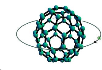
Figure 1: (Color online) Schematic illustration of a charged particle captured by the image potential and orbiting around a buckyball. The radius of the orbit is determined by the dielectric constant within and surrounding the shell as well as the angular momentum quantum number of the captured particle. For semiconducting shells, the localization is strong and the radius of the stable orbit can be a few nanometers. The localization is weak for metallic shells.

The fullerenes are modeled in analogy with the collective excitations in a planar semiconductor two-dimensional-electron-gas. We now consider a spherical shell of radii $R$ whose center is at the origin. The background dielectric constant is $\epsilon_{1}$ for $0<r<R$, and $\epsilon_{2}$ for $r>R$. An electron gas is confined to the surface of the sphere. If a charge $Q$ is located at $(r_{0},\theta_{0},\phi_{0})$ in spherical coordinates, then for $r_{0}>R$, the total electrostatic potential is given by $\Phi_{\rm{tot}}=\Phi_{\rm{ext}}+\Phi_{\rm{ind}}$, where $\Phi_{\rm{ext}}$ is the external potential due to the point particle and $\Phi_{\rm{ind}}$ is the induced potential. The external potential may be expanded in the form

$$\Phi_{\rm{ext}}\left(r,\theta,\phi\right)=4\pi kQ\sum_{LM}\frac{1}{2L+1}\frac{r_{<}^{L}}{r_{>}^{L+1}}Y_{LM}^{\ast}\left(\Omega_{0}\right)Y_{LM}\left(\Omega\right)\ ,$$ (1)

where $k=(4\pi\epsilon_{0})^{-1}$ with $\epsilon_{0}$ the permittivity of free space. Also, $Y_{LM}\left(\Omega\right)$ is a spherical harmonic and $\Omega$ is a solid angle. For $r<R$ we express the total potential in the form

$$\Phi_{\rm{tot}}^{\left(1\right)}\left(r,\theta,\phi\right)=4\pi kQ\sum_{LM}\frac{1}{2L+1}A_{L}r^{L}Y_{LM}\left(\Omega\right),$$ (2)

whereas for $r>R$ we express the induced potential as

$$\Phi_{\rm{ind}}^{\left(2\right)}\left(r,\theta,\phi\right)=4\pi kQ\sum_{LM}\frac{1}{2L+1}B_{L}r^{-\left(L+1\right)}Y_{LM}\left(\Omega\right)\ .$$ (3)

The total potential $\Phi_{\rm tot}^{(2)}(r,\theta,\phi)=\Phi_{\rm ext}(r,\theta,\phi)+\Phi_{\rm ind}^{(1)}(r,\theta,\phi)$ for $r>R$ then becomes

$$\Phi_{\rm{tot}}^{\left(2\right)}\left(r,\theta,\phi\right)=4\pi kQ\sum_{LM}\frac{1}{2L+1}$$ (4)

$$\times \left[\frac{r_{<}^{L}}{r_{>}^{L+1}}Y_{LM}^{\ast}\left(\Omega_{0}\right)+B_{L}r^{-\left(L+1\right)}\right]Y_{LM}\left(\Omega\right)\ .$$

On the surface of the sphere, the boundary conditions are $\Phi_{\rm{tot}}^{\left(1\right)}\left(R,\theta,\phi\right)=\Phi_{\rm{tot}}^{\left(2\right)}\left(R,\theta,\phi\right)$ and $\left.\left[\epsilon_{1}\Phi_{\rm{tot}}^{\left(1\right)}\left(r,\Omega;\omega\right)-\epsilon_{2}\Phi_{\rm{tot}}^{\left(2\right)}\left(r,\Omega;\omega\right)\right]\right|_{r=R}^{\prime}=4\pi k\sigma\left(R,\theta,\phi;\omega\right)\ ,$ where $\sigma\left(R,\theta,\phi;\omega\right)$ is the induced surface charge density on the spherical shell. Expanding $\sigma$ in terms of spherical harmonics and using linear response theory we find

$$\sigma\left(R,\theta,\phi;\omega\right)=-\frac{2kQe^{2}}{R^{2}}\sum_{LM}\frac{1}{2L+1}A_{L}R^{L}\Pi_{L}(\omega)Y_{LM}\left(\Omega\right)\ .$$ (5)

In this equation, $\Pi_{L}(\omega)$ is the SEG polarization function for $L$ an integer and given in terms of the Wigner $3$-$j$ symbol 15 ; 16

$$\Pi_{L}(\omega)=\sum_{\ell\ell^{\prime}}\frac{f_{0}(E_{\ell})-f_{0}(E_{\ell^{\prime}})}{\hbar\omega+E_{\ell^{\prime}}-E_{\ell}}\ (2\ell+1)(2\ell^{\prime}+1)\left(\begin{matrix}l&l^{\prime}&L\cr 0&0&0\cr\end{matrix}\right)^{2}\ ,$$ (6)

where $f_{0}(E)$ is the Fermi-Dirac distribution function and $E_{\ell}=\hbar^{2}\ell(\ell+1)/(2m^{\ast}R^{2})$ with $\ell=0,1,2,\cdots$ and $m^{\ast}$ is the electron effective mass. The induced potential $\Phi_{\rm{ind}}^{\left(2\right)}\left(\bf r;\omega\right)$ outside the spherical shell may be calculated to be

$$\Phi_{\rm{ind}}^{\left(2\right)}\left(\bf r;\omega\right) = 4\pi kQ\sum_{L}\left[\frac{\epsilon_{2}}{\varepsilon_{L}(\omega=0)}-\frac{1}{2L+1}\right]\frac{R^{2L+1}}{r_{0}^{L+1}}$$ (7)

$$\times \frac{1}{r^{L+1}}\sum_{M}Y_{LM}^{\ast}\left(\Omega_{0}\right)Y_{LM}\left(\Omega\right).$$

where $\varepsilon_{L}(\omega)=L\left(\epsilon_{1}+\epsilon_{2}\right)+\epsilon_{2}+(2e^{2}/R)\Pi_{L}(\omega)$ is the dielectric function of the SEG. The force on a charge $Q$ at ${\bf r}_{0}=(r_{0},\phi_{0},\theta_{0})$ is along the radial direction and can be found using $F(r_{0})=-Q\left.\displaystyle\partial\Phi_{\rm{ind}}^{\left(2\right)}({\bf{r}})/\partial r\right|_{{\bf{r}}_{0}}$ yielding

$$F(r_{0})=kQ^{2}\sum_{L}(L+1)\left[(2L+1)\frac{\epsilon_{2}}{\varepsilon_{L}(\omega=0)}-1\right]\frac{R^{2L+1}}{r_{0}^{2L+3}}\ .$$ (8)

The interaction potential energy ${\cal U}_{\rm{im}}(r_{0})$ may now be calculated from

$${\cal U}_{\rm{im}}(r_{0})\equiv\sum_{L}{\cal U}_{\rm{im}}^{(L)}(r_{0})=\frac{1}{2}Q\Phi_{\rm ind}(r_{0},\theta_{0},\phi_{0})$$ (9)

$$= \frac{kQ^{2}}{2r_{0}}\sum_{L}\left[(2L+1)\frac{\epsilon_{2}}{\varepsilon_{L}(\omega=0)}-1\right]\left(\frac{R}{r_{0}}\right)^{2L+1}$$

The effective potential is the sum of the image potential and the centrifugal term and is given by 7 ; 8

$$V\ _{\mbox{eff}}^{(L)}(r_{0},\theta)={\cal U}_{\rm{im}}^{(L)}(r_{0})+\frac{\hbar^{2}\left(L^{2}+L-\frac{1}{4}\right)}{2M^{\ast}(r_{0}\sin\theta_{0})^{2}}\ ,$$ (10)

showing that $V_{\mbox{eff}}^{(L)}$ is not spherically symmetric. In this notation, $M^{\ast}$ is the mass of the captured charged particle in an orbital state with angular momentum quantum number $L$. In Fig. 2(a), we calculated $V_{\mbox{eff}}^{(L)}(r_{0},\theta)$ as a function of $r_{0}$, for chosen $L,\ R$. Also, for the background dielectric constant, we chose $\epsilon_{1}=2.4$, corresponding to graphite, and $\epsilon_{2}=1$. The electron effective mass used in calculating the polarization function $\Pi_{L}$ in Eq. (6) was $m=0.25m_{e}$ where $m_{e}$ is the bare electron mass, and the Fermi energy $E_{F}=0.6\ eV$. The orbiting particle effective mass $M^{\ast}=m_{e}$. Figure 2(b) shows how the peak values of the effective potential depend on radius. Of course, the height of the peak is linked to the localization of the particle in orbit. In Fig. 3, the ground and three lowest excited state wave functions are plotted for the effective potential $V_{\rm eff}^{(L)}$ when $L=2$ in Fig. 2(a).

Figure 2: (Color online) (a) The effective potential $V_{\rm eff}$ between a charged particle and a spherical shell is shown for a number of angular momenta $L$. The radius of the sphere is $R=1$ nm and we chose $\epsilon_{1}=2.4,\ \epsilon_{2}=1$. In (b), the height of the peak in the effective potential appearing in (a) is plotted as a function of the radius.

The value of the angular momentum quantum number $L$ as well as the curvature of the surface of these complex carbon structures clearly plays a crucial role in shaping the effective potential. Generally, the form for the $L$-th term may be expressed as $V_{\rm eff}^{(L)}(r_{0})=-\alpha_{L}r_{0}^{-2(L+1)}+\beta_{L}r_{0}^{-2}$, where $\alpha_{L}$ and $\beta_{L}$ are due to the image potential and centrifugal force, respectively. The coefficient $\alpha_{L}$ is always positive whereas $\beta_{L}$ is only negative for $L=0$. This power-law behavior ensures that no matter what values the two coefficients may have the image term dominates the centrifugal term, leading to a local maximum in the effective potential. This is unlike the behavior for a cylindrical nanotube where the image term is logaritmic, due to the linear charge distribution, and may be dominated by the $r_{0}^{-2}$ centrifugal term, leading to a local minimum instead. Consequently, capturing and localizing a charged particle by the image potential of spherical conductors and dielectrics is fundamentally different from that for a cylindrical nanotube. For the sphere, as shown in Fig. 3, the wave function is more localized around the spherical shell within its effective potential, i.e., the wave function is not as extended . Additionally, the confinement of the charged particle is close to the spherical surface.

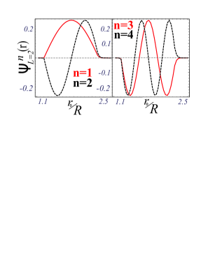
Figure 3: (Color online) The wave functions for the ground state ($n=1$) and first three excited states ($n=2,3,4$) are plotted for the effective potential $V_{\rm eff}$ between a charged particle and a spherical shell when $L=2$. We chose $\epsilon_{1}=2.4,\ \epsilon_{1}=1$ and $R=1\;nm$

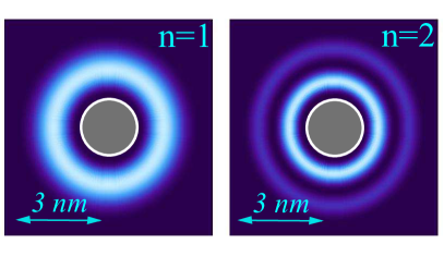
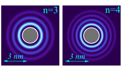
Figure 4: (Color online) Probability density plots for $|\Psi_{L,n}(r_{0})|^{2}/r_{0}^{2}$ when $L=2$ and $n=1,2$ (upper panel) as well as $n=3,4$ (lower panel), where $n$ labels the eigenstates, for a spherical shell of radius $R=10$ Å. The wave function $\Psi_{L,n}(r_{0})$ is a solution of the one-dimensional Schrödinger equation with effective potential $V_{\mbox{eff}}(r_{0},\theta=\pi/2)$ shown in Fig. 2. We chose $\epsilon_{1}=2.4$ inside the ball, whose outline is shown as a thin circle, and $\epsilon_{2}=1$ in the surrounding medium.

The choice for the radius does render some crucial changes in $V_{\rm eff}^{(L)}$ to make a difference in the location and height of the peak. However, only the higher-lying localized states are affected. In Fig.  2, we show how the peak height changes as $L$ is varied. Additional numerical results corresponding to $\epsilon_{1}\gg\epsilon_{2}$ have shown that a spherical metallic shell has a reduced potential peak for confining the captured charge. Thus, the spherical metallic shell is not as susceptible for particle confinement in highly excited states as the metallic nanotube. 7 ; 8 ; 8b This indicates that the dimensionality plays a non-trivial role in formation of image states and their spatial extension near the surface of the nanometer-size graphitic structure. This direct crossover from a one-dimensional to a three-dimensional regime is not determined by polarization effects for the structure in the metallic limit since in the limit $\epsilon_{1}\to\infty$ in Eq. (8), the $\Pi_{L}(\omega)$ term makes no contribution. The difference is due entirely to the geometrical shape in the metallic regime where graphitic plasmons fail to develop. For finite values of $\epsilon_{1}$, we encounter the regime where excited particles contribute through the polarization function $\Pi_{L}(\omega)$ defined in Eq. (6). The behavior of plasmon excitation as a function of angular momentum quantum number $L$ for fullerenes resembles in all respects the long wavelength ($q\to 0$) limit of carbon nanotubes 18 ; 19 ; 20 . Furthermore, in the case of the low-frequency $\pi$- plasmons in carbon nanotubes, a surface mode may develop for large $q$, due to the difference in the values for the dielectric constants within the graphitic structure and the surrounding medium 21 .

Since the polarization function $\Pi_{L}(\omega)$ vanishes identically for $L=0$, the attractive part of the effective potential is only significantly modified by screening for a fast-rotating electron. This behavior at zero angular momentum differs from tubular-shaped image states for single-walled carbon nanotubes which are formed in a potential isolated from the tube 7 . The large angular momentum image states for spheres may be probed by femtosecond time-resolved photoemission 8cc+ . Our formalism shows that considering photoionization from various levels of C₆₀, the Coulomb interaction between an external charge and its image is screened by the statically stretched SEG through the dielectric function $\epsilon_{L}(\omega=0)$. The polarization of the medium $\Pi_{L}$ which is driven by the electrostatic interaction is generated by particle-hole transitions across the Fermi surface. The polarization also determines the Ruderman-Kittel-Kasuya-Yosida (RKKY) interaction energy between two magnetic impurities as well as the induced spin density due to a magnetic impurity.

Increasing radius, the position of the peak moves closer to the sphere as $R^{-1/(2L)}$. In the absolute units, the position of the peak depends as $r_{0}^{(peak)}\backsim R^{1-1/(2L)}$. The typical distances from the surface are between $1.3\ R$ and $1.5\ R$. Figure 2 (b) demonstrates how the potential peaks (corresponding to the local maximum for the $V_{\rm eff}$) depend on the radius of the buckyball for various angular momentum quantum number $L$. Clearly, we see that the potential peak decreases with increased radius leading us to conclude that confinement is strongest for smaller buckyballs and particles with large angular momentum. For the nanotube, increasing $L$ leads to a reduced local minimum in the effective potential and the ability to localize the charge 7 . Approximately, the curves may be fitted analytically to $\backsim 1/R$ for all considered values of $L$. However, we found that a better fit for $L>5$ would be of the form $c_{1}/R+c_{2}/R^{2}$ where $c_{1},c_{2}$ are constants.

For increased $\epsilon_{1}$, i.e., the metallic limit with $\epsilon_{1}\gg\epsilon_{2}$, we have $\epsilon_{L}\backsimeq\epsilon_{1}L$, so that the coefficient $\left((2L+1)[\epsilon_{2}/\epsilon_{L}]-1\right)\to-1$. In the case of dielectric constant $\epsilon_{1}\sim 2.4$ for the buckyball, the above mentioned coefficients lie within the range from $-0.4$ to $-0.9$ and decreases with increasing $L$. Consequently, for the transition to the metallic limit, these coefficients are more affected for states with large $L$. So, we may conclude that $\epsilon_{1}$ has little effect on the position and height of the peak in the effective potential. In fact, for the metallic case, the peak is observed to be slightly further away from the center (very little difference $\sim 1.37\ R$ compared to $\sim 1.31\ R$ for $R=1\;nm$). The height of the peak is only slightly decreased in the metallic case ($0.24$ compared to $0.27$ in the case of fullerenes). These numbers are provided for fixed $L$ and the unit of energy is the same as that in Fig. 2.

Regarding the wave functions and density plots, Figs. 3, and 4 demonstrate the wave function of a bounded electron trapped between the infinite hard wall of the sphere and the potential peak. First, we note that we obtained qualitatively similar behavior for different values of $L$, so the electron states corresponding to the potentials with different angular momenta are almost the same. We clearly see that the electron wave functions are not exactly localized in the ”potential well” due to the asymmetry of the boundary conditions, i.e., infinitely high wall on the left and the effective potential profile on the right-hand side. The wave functions corresponding to $L=0$ are extremely delocalized due to the relatively shallow potential. The fact that the effective potential is not spherically symmetric means that for arbitrary angle $\theta$, we must solve a three-dimensional Schrödinger equation. However, for trajectories parallel to the $x-y$ plane when the angle $\theta$ is a constant of motion, the problem reduces to a quasi-one-dimensional Schrödinger equation involving the radial coordinate. In our calculations, we set $\theta=\pi/2$ so that the captured charge is moving in the equatorial plane. For this, the centrifugal term is weakest compared to the image potential, but still affords us the opportunity to see its effect on localization. The density plots in Fig. 4 show that the innermost ring is substantially brighter than the outer rings. This is a consequence of the presence of the $r_{0}^{-2}$ factor in the electron probability function. In contrast, the corresponding plots for the nanotube 8b do not have the innermost ring so much brighter than the outer rings because of the fact that the density function in that case depends on inverse distance of the charge from the center of the cylinder instead. This is another unusual specific feature of the considered geometry and indicates that the captured charge is more strongly localized for the spherical shell closest to the surface for the sphere than the cylindrical nanotube. The lowest bound states for Fig. 3 are in the range from $-10$ to about$-100$ meV, with first few excited states lying very close to the ground state energy. Of course, the bound state energies may be adjusted by varying the radius $R$ since our calculations have shown that the peak potential decreases as a power function with increasing radius. This property allows considerable manipulation of a captured electron and its release to a source of holes for recombination and release of a single photon whose frequency and polarization are linked to the electron. This single-photon source may have variable frequency with a broad range of applications in quantum information where the message is encoded in the number of photons transmitted from node to node in an all-optical network. Gate operations are performed by the nodes based on quantum interference effects between photons which cannot be identified as being different. The low frequency photons could be in the infrared which is most useful range for telecommunications. Another, more general, practical application and technological use of such unique quantum states would be to quantum optical metrology of high-accuracy and absolute optical measurements.

- (1) E. Osawa, Kagaku 25, 854 (1970).
- (2) Joseph F. Anacleto, Michael A. Quilliam, Anal. Chem. 65, 2236 (1993).
- (3) H.W. Kroto, J. R. Heath, S. C. O’Brien, R. F. Curl, and R. E. Smalley, Nature 318, 162 (1985);
- (4) S Iijima, Journal of Crystal Growth 50, 675 (1980).
- (5) P.R. Buseck, S.J. Tsipursky, R. Hettich, Science 257, 215 (1992).
- (6) J. Cami, J. Bernard-Salas, E. Peeters, S. E.Malek, Science 329, 180 (2010).
- (7) C. A. Poland, et al., Nature Nanotechnology 3, 423 (2008).
- (8) Brian E. Granger, Petr Král, H.R. Sadeghpour, and Moshe Shapiro, Phys. Rev. Lett. 89, 135506 (2002).
- (9) Godfrey Gumbs, Antonios Balassis, and Paula Fekete, Phys. Rev. B 73, 075411 (2006).
- (10) S. Segui, C. Celedon L pez, G. A. Bocan, J. L. Gervasoni, and N. R. Arista, Phys. Rev. B 85, 235441 (2012).
- (11) K. Schouteden, A. Volodin, D. A. Muzychenko, M. P. Chowdhury, A. Fonseca, J. B. Nagy, and C. Van Haesendonck, Nanotechnology 21, 485401 (2010).
- (12) Matthew A. McCune, Mohamed E. Madjet, and Himadri S. Chakraborty, Journal of Physics B: Atomic, Molecular and Optical Physics 41, 201003 (2008).
- (13) M. Zamkov, N. Woody, S. Bing, H. S. Chakraborty, Z. Chang, U. Thumm, and P. Richard, Phys. Rev. Lett. 93, 156803 (2004).
- (14) Silvina Segui, Gisela A. Bocan, N stor R. Arista, and Juana L. Gervasoni, Journal of Physics: Conference Series 194, 132013 (2009).
- (15) Anne Goodsell, Trygve Ristroph, J. A. Golovchenko, and Lene Vestergaard Hau, Phys. Rev. Lett. 104, 133002 (2010).
- (16) V. l. .A. Margulis and E. E. Muryumin, Physica B: Condensed Matter 390, 134 (2007).
- (17) P. M. Echenique and J. B. Pendry, J. Phys.: Condens. Matter 11, 2065 (1978).
- (18) J. Lehmann, M. Merschdorf, A. Thon, S. Voll, and W. Pfeiffer, Phys. Rev. B 60, 17037 (1999).
- (19) 19 I. Kinoshita, D. Ino, K. Nagata, K. Watanabe, N. Takagi, and Y. Matsumoto, Phys. Rev. B 65, 241402(R) (2002).
- (20) V. M. Silkin, J. Zhao, F. Guinea, E. V. Chulkov, P. M. Echenique, and H. Petek, Phys. Rev. B80, 121408(R) (2009).
- (21) Godfrey Gumbs, D. Huang, and P. M. Echenique, Phys. Rev. B 79,035410 (2009).
- (22) J. Zhao, M. Feng, J. Yang, and H. Petek, ACS Nano 3, 853 (2009).
- (23) Lu-Jing Hou and Z. L. Miskovic, Phys. Rev. E 77, 046401 (2008).
- (24) Takeshi Inaoka, Surface Science 273, 191 (1992) .
- (25) P. Longe, Solid State Communications 97, 857 (1996).
- (26) J. Tempere, I. F. Silvera, and J. T. Devreese, Phys. Rev. B65, 195418(2002).
- (27) J. Tempere, I.F. Silvera, J.T. Devreese, Surface Science Reports 62, 159 (2007).
- (28) Constantine Yannouleas, Eduard N. Bogachek, and Uzi Landman, Phys. Rev. B53, 10 225 (1996).
- (29) Carsten Bingel, Chemische Berichte 126, 1957 (1993).
- (30) Godfrey Gumbs and G. R. Aizin, Phys. Rev. B 65, 195407 (2002).
- (31) M.F. Lin and W.K. Kenneth Shung, Phys. Rev. B 47, 6617 (1993).
- (32) M.F. Lin and W.K. Kenneth Shung, Phys. Rev. B 48, 5567 (1993).
- (33) A. Bahari and A. Mohamadi, Nuclear Instruments and Methods in Physics Research Section B: Beam Interactions with Materials and Atoms 268, 3331 (2010).