A remarkably simple and accurate method for computing the Bayes Factor from a Markov chain Monte Carlo Simulation of the Posterior Distribution in high dimension

Abstract

Weinberg, (2012) described a constructive algorithm for computing the marginal likelihood, $Z$, from a Markov chain simulation of the posterior distribution. Its key point is: the choice of an integration subdomain that eliminates subvolumes with poor sampling owing to low tail-values of posterior probability. Conversely, this same idea may be used to choose the subdomain that optimizes the accuracy of $Z$. Here, we explore using the simulated distribution to define a small region of high posterior probability, followed by a numerical integration of the sample in the selected region using the volume tessellation algorithm described in Weinberg, (2012). Even more promising is the resampling of this small region followed by a naive Monte Carlo integration. The new enhanced algorithm is computationally trivial and leads to a dramatic improvement in accuracy. For example, this application of the new algorithm to a four-component mixture with random locations in 16 dimensions yields accurate evaluation of $Z$ with 5% errors. This enables Bayes-factor model selection for real-world problems that have been infeasible with previous methods.

Keywords: Bayesian computation, marginal likelihood, algorithm, Bayes factors, model selection

1 Introduction

Bayesian methods hold the promise of selecting general models with different dimensionality and unrelated structure. For example, consider a collection of such models, $\mathcal{M}=\{M_{1},M_{2},\ldots M_{m}\}$, proposed to describe the data ${\bf D}$. Each model $M_{j}$ is described by parameter vectors $\boldsymbol{\theta}_{j}\in\mathbb{R}^{d_{j}}$ where $d_{j}=\dim(\boldsymbol{\theta}_{j})$. Bayes theorem gives the posterior probability density for each model:

$$P(M_{j}|{\bf D})=\frac{P(M_{j})P({\bf D}|M_{j})}{P({\bf D})}$$ (1)

where $P(M_{j})$ is the prior probability of Model $j$, $P({\bf D})$ is an unknown normalization and

$$P({\bf D}|M_{j})=\int d\boldsymbol{\theta}_{j}\,P(\boldsymbol{\theta}_{j}|M_{j})P({\bf D}|\theta_{j},M_{j})$$ (2)

is the marginal likelihood for Model $j$. The posterior odds of any two models $j,k\in[1,m]$ is then

$$\frac{P(M_{j}|{\bf D})}{P(M_{k}|{\bf D})}=\left[\frac{P(M_{j})}{P(M_{k})}\right]\left[\frac{P({\bf D}|M_{j})}{P({\bf D}|M_{k})}\right],$$ (3)

now independent of the normalization $P({\bf D})$. The first term on the right-hand side describes the odds ratio from prior knowledge and the second term is the Bayes factor. In most cases, the set of models is given a counting measure; the posterior odds ratio is then equal to the Bayes factor. If $P(M_{j}|{\bf D})\gg P(M_{k}|{\bf D})$ for all $k\in[1,m],k\not=j$, Model $j$ best explains the data out of all the proposals in $\mathcal{M}$.

The Bayes factor requires the computation of the marginal likelihood for each model. Analytic computation is almost never possible and direct evaluation by numerical quadrature is almost never feasible for models of real-world dimensionality and complexity. This has led to a variety of approximations based on special properties of the models or their posterior distributions. For example, a smooth unimodal distribution that is well-represented by a multidimensional normal distribution can be evaluated by Laplace approximation (e.g. Kass and Raftery,, 1995). The dimensionality for nested models can be effectively lowered as described in DiCicio et al., (1997). Chib and Jeliazkov, (2001) describe an efficient approach for models amenable to block sampling. A number of astronomical problems of current interest (e.g. Yoon et al.,, 2011; Lu et al.,, 2011, 2012) do not fit into these categories and require explicit methods.

Motivated by these problems, Weinberg, (2012) explored the direct use of MCMC samples to compute the marginal likelihood and proposed two algorithms. In essence, both use the MCMC sample to identify the important regions of parameter space. The first algorithm modifies the harmonic-mean approximation to remove the low-probability tail of the distribution that dominates the error. However, if the harmonic mean integral itself is improper, as it typically is for problems with weakly informative prior distributions, this algorithm will fail. The second algorithm assigns probability to a tree partition of the sample space and performs the marginal likelihood integral directly. This algorithm is consistent for all (proper) posterior distributions. Additional recent applications have suggested a number of important extensions to these ideas, which is what we will explore in this paper. We will begin in §2 with a intuitive motivation and review of Weinberg, (2012).

2 The Main Point

This contribution focuses on a further extension of the second algorithm that dramatically improves its feasibility in a variety of cases. Let $\Omega$ be the MCMC sample of the desired posterior probability. The central point of Weinberg, (2012) is the following: the marginal likelihood $P({\bf D}|M_{j})$ is defined by

$$P({\bf D}|M_{j})\int_{\Omega_{s}}dP(\boldsymbol{\theta}_{j}|{\bf D})=\int_{\Omega_{s}}d\boldsymbol{\theta}_{j}\,P(\boldsymbol{\theta}_{j}|M_{j})P({\bf D}|\boldsymbol{\theta}_{j},M_{j})$$ (4)

where the set $\Omega_{s}\subset\Omega$ may be chosen to optimize the numerical evaluations of the integrals in equation (4). Evaluated by Monte Carlo sampling, the integral on the left-hand side of equation (4) is simply the fraction of points in $\Omega_{s}$ relative to the number in $\Omega$. The integral on the right-hand side of equation (4) is performed by quadrature after the measure is assigned by associating tessellated volume elements $v({\omega_{i}})$ in $\mathbb{R}^{d_{j}}$ to each point or group of points $\omega_{i}$ in $\Omega$. The unity of all subvolumes $v_{i}\equiv v(\omega_{i})$ in the tessellation is a convex hull in $\mathbb{R}^{d_{j}}$. By construction, the MCMC algorithm provides samples such that $\int_{\omega_{i}}d\boldsymbol{\theta}_{j}P(\boldsymbol{\theta}_{j}|{\bf D})\approx P({\bar{\boldsymbol{\theta}}}|{\bf D})v_{i}\approx\mbox{constant}$ for some ${\bar{\boldsymbol{\theta}}}\in\omega_{i}$. Therefore, relatively small values of $P({\bar{\boldsymbol{\theta}}})$ will be associated with relatively large values $v_{i}$, and, therefore, will contribute most of the variance to the resulting quadrature on the right-hand side of equation (4).

This motivates seeking subsets $\Omega_{s}\subset\Omega$ that preserve the measure defined by the tessellation that minimizes the variance of equation (4). A particular solution is intuitively obvious: successively peel the subvolumes on the hull until the volumes $v_{i}$ are sufficiently small that $P(\boldsymbol{\theta}_{j}|{\bf D})$ varies slowly across $v_{i}$ while preserving the condition $|\Omega_{s}|\gg 1$ so that the error in the integral on the left-hand side of equation (4) remains small. Below, we explore three extensions to this approach whose goals are optimizing the choice of $\Omega_{s}$ to accurately and efficiently evaluate equation (4). In §3.1, we try the peeling approach. In §3.2, we identify an easy to tessellate volume near the posterior mode containing the subset $\omega_{s}$ and retessellate this volume. In addition, rather than using the original MCMC sample, the new subvolume identified from the sample can be resampled with a new more efficient sampling function, improving the results.

These proposed extensions do not circumvent the curse of dimensionality (Bellman,, 2003); we still are required to sample a high-dimensional space. However, the approach described above allows us to choose a domain that results in the most accurate integral with the smallest number of samples.

3 Using MCMC for importance sampling choice of the subdomain

3.1 Volume peeling

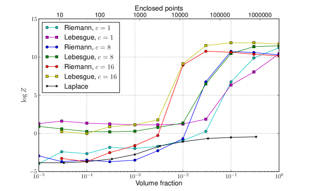
Figure 1: Values of $\log Z$ obtained with the volume-peeling strategy compared with both volume tessellation algorithms for a chain of three million states. The lower axis (upper axis) shows the enclosed volume fraction (number of points) in the ‘peeled’ subvolume. The Laplace approximation applied to a subset of the entire sample (using the upper axis) is shown for comparison. The true value is $\log Z=0$.

We tried two implementations of volume peeling. Both define the geometric center of mass and slowly decrease the scale of the self-similar volume in $\mathbb{R}^{d_{j}}$. In the first implementation, We eliminated all subvolumes $v_{i}$ outside of or containing the boundary of the scaled self-similar volume. In the second, we computed the set $\Omega_{s}$ contained within the new boundary and recomputed the tessellation. The latter is slightly more accurate than the former but requires a new tessellation. We adjust the scale factor to retain a fixed number of points $N$, and, therefore, limit the error in the left-hand side of equation (4) to a root variance of approximately $1/\sqrt{N}$.

The results of applying the volume peeling strategy to a Markov-chain-sampled normal distribution in twelve dimensions is illustrated in Figure 1. For the tessellation, we use a k-d tree with a round-robin geometric bisection, sometimes known as the orthogonal recursive bisection (ORB) tree. This tree recursively subdivides the cells into equal subvolumes, one dimension at a time. The recursion stops when the next division produces cells with occupation numbers below the target size $c$. This algorithm prevents cells with extreme axis ratios but the cells will not have the same number of counts. For this test, we adopt a target cell count of $c=8$. The figure shows both the Riemann ($\mbox{VTA}_{1}$) and Lebesgue ($\mbox{VTA}_{2}$) variants for estimating the integrals in equation (4), as in described in Weinberg, (2012). The Riemann computation uses the median value of the posterior probability in each cell to compute the contribution to the Riemann integral:

$$\int d\boldsymbol{\theta}\,P(\boldsymbol{\theta}|{\bf D})\approx\sum_{j}v(\omega_{j})\operatorname{median}\{P(\boldsymbol{\theta}_{k}|{\bf D})\}$$ (5)

where $\mathbf{\theta}_{k}\in\omega_{j}$ and $v(\omega_{j})$ is the hypervolume in the subdomain $j$ (i.e. the cell). The Lebesgue computation assigns the hypervolume by probability according to the monotone function $f(P)$ as follows:

$$v(\omega_{j};P)\equiv\int_{P>P_{k};k\in\omega_{j}}d\boldsymbol{\theta}\approx\frac{v(\omega_{j})}{|\omega_{j}|}\sum_{k\in\omega_{j}}\begin{cases}1&\mbox{if}\,P\geq P_{k+1}\\ \frac{f(P)-f(P_{k})}{f(P_{k+1})-f(P_{k})}&\mbox{else if}\,P_{k+1}>P>P_{k},\\ 0&\mbox{otherwise}\end{cases}$$ (6)

where we assume that $P_{l}>P_{k}$ if $l>k$. For the computations here, we choose $f(x)=x$. The Lebesgue integral is then approximated as

$$\int d\boldsymbol{\theta}\,P(\boldsymbol{\theta}|{\bf D})\approx\sum_{k}\frac{1}{2}\left(P_{k+1}-P_{k}\right)\left(\sum_{j}v(\omega_{k+1})+\sum_{j}v(\omega_{k})\right).$$

The Riemann and Lebesgue constructions differ, even in the limit $c=1$.

Figure 1 demonstrates that the choice of an appropriate subdomain results in acceptable approximations to the marginal likelihood. In all cases, the sparsely sampled tails of the distribution coupled with regions of empty volume bias the evaluation of $Z$ upward. As the volume is peeled from the outside, the offset from the true value $Z=1$ ($\log Z=0$) decreases dramatically, as expected. All evaluations are for a fixed chain size. Therefore, larger values of $c$ imply lower spatial resolution. In addition, as $c$ increases and the cell width approaches the characteristic scale of the posterior distribution, the variance of $P$ in the cell increases and the approximations in equations (5) and (6) become inaccurate. On the other hand, a small volume fraction constrains the sampled region to the peak of the distribution. Near the peak, the variance of $P$ decreases and accuracy is recovered. This explains the shift to smaller volume fraction required to obtain accuracy with higher $c$ in Figure 1. Both variants are biased in the limit of small volume fractions; the Lebesgue (Riemann) method is biased high (low). The Lebesgue (Riemann) variant with $c\geq 8$ ($c=1$) has the smallest bias. The Lebesgue variant has the lowest bias overall.

The underestimation of $Z$ by the Riemann algorithm makes intuitive sense; the distribution of probability values in each cell will be exponentially skewed toward higher values. Using the median value as the representative value for the cell will tend to underestimate the cell’s true contribution. The overestimation of $Z$ by the Lebesgue owes to the linear assignment of probability to volume in the measure function (our choice of $f(x)$ in eq. 6); the true value of $f(x)$ is likely to be some convex-up function.

We show the Laplace approximation for comparison. We use the same number of enclosed points implied by the volume fraction for the Riemann and Lebesgue variants but randomly sampled from the entire chain with no volume restriction. As expected, the Laplace approximation converges to the true value for a large sample from a multivariate normal distribution. Similar results obtain for lower and higher dimensionality. We have checked this up to $d=16$.

Applying the Lebesgue variant of the volume tessellation algorithm (VTA) to an appropriately ‘peeled’ volume for a unimodal distribution provides a usefully accurate evaluation of the marginal likelihood. Now imagine a bimodal distribution with two widely separated modes. The volume peeling strategy will fail miserably: the central fractional volume will tend to sit in the poorly sampled desert between the two modes. An adaptive approach is needed.

3.2 Identification of the posterior mode

The previous family of subdomain selections relies purely on the shape of the enclosing volume. In general, this algorithm will not center the subdomain on the shallowest part of the posterior distribution. For a worst-case counterexample, consider two equally shaped but widely separated spherical modes in parameter space. The algorithm in §3.1 will eliminate the peaks and retain the tails of both modes. This leads to a worse estimate than the original estimate based on the full posterior sample.

This counterexample suggests the following alternative approach:

1. Set the center to the location of the parameter point $\boldsymbol{\theta}_{k}$ with the maximum value of the posterior probability: $P(\boldsymbol{\theta}_{k}|{\bf D})>P(\boldsymbol{\theta}_{j}|{\bf D})$ for all $j\not=k,j\in[1,\ldots,N]$

2. Compute the shape of the hyperrectangle initially from the parameter ranges of the entire sample: $\sigma_{0r}=\max\{\theta_{1r},\ldots,\theta_{Nr}\}-\min\{\theta_{1r},\ldots,\theta_{Nr}\}$.

3. Let $q$ count the number of iterations and set $q=0$ to start.

4. Compute the distances of the sample from $\boldsymbol{\theta}_{k}$: $d_{j}^{2}=\sum_{r}(\theta_{jr}-\theta_{kr})^{2}/\sigma_{qr}^{2}$

5. Let ${\bar{d}}$ be the $M^{\mbox{th}}$ distance in the sorted list of distances. Choose $M$ large enough to achieve a sufficiently small variance in ${\bar{d}}$ (e.g. $M=10^{3}$). The enclosing hyperrectangle now has the coordinates $\theta_{min,r}=\theta_{kr}-\sigma_{0r}{\bar{d}}$ and $\theta_{max,r}=\theta_{kr}+\sigma_{0r}{\bar{d}}$.

6. Increment $q$ and recompute the shape of the hyperrectangle from the variance of the entire sample, $\sigma_{qr}^{2}=\sum_{j}(\theta_{jr}-\theta_{kr})^{2}$ for $\boldsymbol{\theta}_{j}\in[\boldsymbol{\theta}_{min},\boldsymbol{\theta}_{max}]$. Repeat Steps 4–5.

7. Steps 4–6 may be iterated until converged, if desired.

8. Finally, tessellate the volume defined by these $M$ points and compute the right-hand side of equation (4)

This algorithm significantly improves the marginal likelihood computations, resulting in errors in the log of the marginal likelihood of several tens of percent, i.e. $|\delta\log P({\bf D}|M_{j})|<0.2$. However, the bias in these estimates appears to decrease slowly with sample size. This bias appears to result from large changes in $P(\boldsymbol{\theta}_{j}|{\bf D})$ across the subvolumes. To test this speculation, we replaced Step 8 in the algorithm listed in §3.2 by a uniform resampling of the hyperrectangle. A uniform sampling over the volume prevents the volume of the cells growing as the probability value decreases and results in a strong suppression of the bias. A sampling function with less variance than uniform over the sample volume might lead to better accuracy while still suppressing the bias, but we have not investigated this possibility.

3.3 Test problems

Here, the original and new algorithms are applied to the following four test distributions constructed from one or more normal components with a variance $\sigma^{2}=0.003$ and centered in the unit hypercube of dimensionality $d$. The centers for the test distributions are as follows:

1. A single distribution with center ${\bar{x}}=(0.5,\ldots,0.5)$.

2. Two separated distributions with centers ${\bar{x}}_{1}=(0.2,0.2,0.5,\ldots,0.5)$ and ${\bar{x}}_{2}=(0.8,0.8,0.5,\ldots,\allowbreak 0.5)$ with corresponding weights $w_{1}=0.6,w_{2}=0.4$. This distribution simulates two widely separated modes. Figure 2 (left) shows the distribution marginalized in all but the first two dimensions for $d=8$ and for a MCMC-generated sample of $10^{5}$ points.

3. Two overlapping distributions with centers ${\bar{x}}_{1}=(0.4,0.4,0.5,\ldots,0.5)$ and ${\bar{x}}_{2}=(0.6,0.6,0.5,\ldots,\allowbreak 0.5)$ with corresponding weights $w_{1}=0.6$, $w_{2}=0.4$. This distribution a distribution with two local maxima on a common pedestal. Figure 2 (right) shows shows the distribution marginalized in all but the first two dimensions for $d=8$ and $10^{5}$ MCMC points.

4. Four randomly-oriented distributions with their centers uniformly selected from the hypercube $[0.5-2\sigma,0.5+2\sigma]^{d}$ at random with Dirichlet distributed weights and shape parameter $\alpha=1$. This produces an asymmetric distribution with multiple maxima connected by “necks” of varying amplitude and emulates features of posterior distributions from parametric models found in practice (e.g. Lu et al.,, 2012). Figure 3 shows the distribution in pairs of marginal variables for $d=8$.

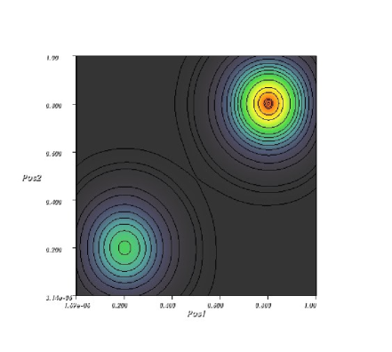
(a) separated

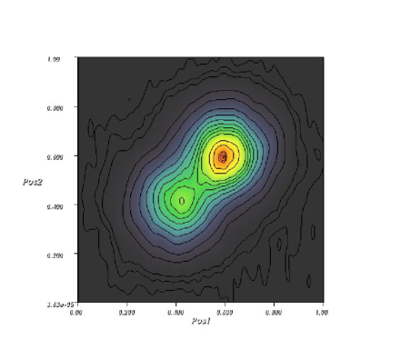
(b) overlapped

Figure 2: Marginalization of two-component Gaussian distribution in 8 dimensions using $10^{5}$ MCMC samples for Test Distribution 2 (left) and Test Distribution (3) (right). The contour levels are 0.001, 0.005, 0.01, 0.05, 0.1, 0.2, 0.3, 0.4, 0.5, 0.6, 0.7, 0.8, 0.9, 0.95, 0.99, 0.995, 0.999.

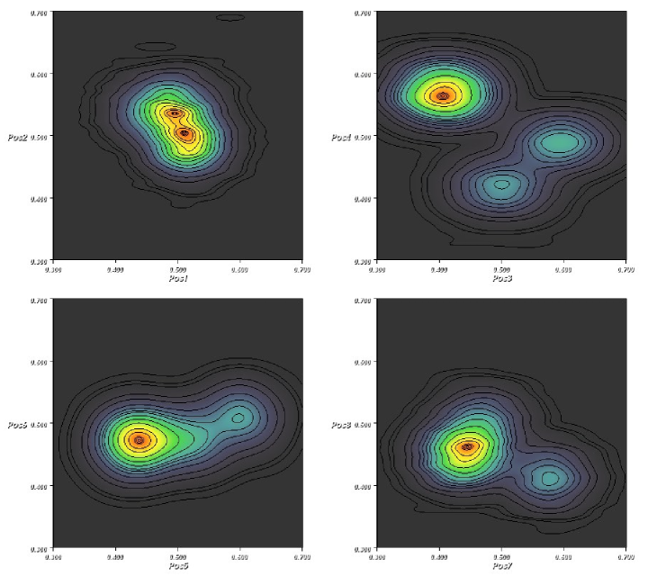
Figure 3: Marginalized distribution of the four-component Gaussian distribution with randomly chosen centers in 8 dimensions using $10^{5}$ MCMC samples for Test Distribution 4. The four panels describe different projections as indicated by the axis labels. Contour levels are as described in Fig. 2.

Table 1: Error in marginal likelihood values: original algorithm

Model		Error in $\log Z$
		100% Volume, $c=8$			0.1% volume, $c=8$		0.1% volume, $c=16$
Type	d	$\hbox{VTA}_{1}$	$\hbox{VTA}_{2}$	Laplace	$\hbox{VTA}_{1}$	$\hbox{VTA}_{2}$	$\hbox{VTA}_{1}$	$\hbox{VTA}_{2}$
1. Single	4	$2.68$	$0.55$	$0.00$	$-3.11$	$-0.07$	$-3.21$	$-0.08$
	8	$6.38$	$5.03$	$-0.08$	$-2.56$	$0.06$	$-2.70$	$0.01$
	12	$9.33$	$10.24$	$-0.29$	$-3.49$	$0.29$	$-1.59$	$1.13$
	16	$14.10$	$11.58$	$0.66$	$13.22$	$15.59$	$12.75$	$14.96$
2. Separated	4	$10.46$	$9.10$	$9.33$	$\infty$	$\infty$	$\infty$	$\infty$
	8	$10.78$	$9.73$	$8.40$	$\infty$	$\infty$	$\infty$	$\infty$
	12	$11.07$	$8.70$	$1.12$	$\infty$	$\infty$	$\infty$	$\infty$
	16	$13.00$	$10.51$	$3.49$	$\infty$	$\infty$	$\infty$	$\infty$
3. Overlapped	4	$3.08$	$0.76$	$0.49$	$-4.60$	$-0.03$	$-3.55$	$-0.13$
	8	$6.51$	$5.35$	$0.12$	$-3.35$	$0.29$	$-3.55$	$0.16$
	12	$9.44$	$10.11$	$-0.71$	$-3.61$	$0.40$	$-3.78$	$0.20$
	16	$12.65$	$13.87$	$-0.64$	$5.36$	$6.38$	$14.25$	$15.76$
4. Random	4	$-2.50$	$-0.01$	$4.76$	$-2.51$	$0.02$	$-4.26$	$0.12$
	8	$-1.37$	$0.67$	$4.41$	$-1.13$	$0.92$	$-1.92$	$0.99$
	12	$1.37$	$3.81$	$4.40$	$7.99$	$9.79$	$-1.24$	$2.42$
	16	$-15.76$	$16.57$	$4.67$	$14.91$	$16.20$	$14.33$	$17.06$

Table 2: Error in marginal likelihood values: important region

Model		Error in $\log Z$
		Subregion			Resampled
Type	d	$\hbox{VTA}_{1}$	$\hbox{VTA}_{2}$	Mean	$\hbox{VTA}_{1}$	$\hbox{VTA}_{2}$	Mean
1. Single	4	$-0.090$	$-0.093$	$-0.0092$	$-0.014$	$-0.023$	$-0.016$
	8	$-0.667$	$-1.097$	$-0.676$	$-0.081$	$-0.121$	$-0.0954$
	12	$-0.746$	$-1.178$	$-0.795$	$0.056$	$-0.021$	$-0.018$
	16	$-0.43$	$-1.08$	$-0.48$	$-0.13$	$-0.12$	$-0.09$
2. Separated	4	$-0.472$	$-0.484$	$-0.475$	$-0.040$	$-0.032$	$-0.036$
	8	$-0.710$	$-1.089$	$-0.703$	$-0.115$	$-0.163$	$-0.140$
	12	$-0.667$	$-1.41$	$-0.717$	$-0.121$	$-0.200$	$-0.139$
	16	$-0.702$	$-0.702$	$-0.571$	$0.027$	$-0.161$	$-0.141$
3. Overlapped	4	$-0.389$	$-0.389$	$-0.391$	$0.108$	$0.102$	$0.105$
	8	$-0.002$	$-0.076$	$-0.020$	$0.075$	$0.016$	$0.053$
	12	$-0.445$1	$-0.548$	$-0.515$	$0.070$	$-0.021$	$0.0178$
	16	$-0.455$	$-0.846$	$-0.520$	$0.200$	$-0.031$	$0.048$
4. Random	4	$-0.460$	$-0.466$	$-0.463$	$0.099$	$0.044$	$0.044$
	8	$-0.456$	$-0.502$	$-0.499$	$0.021$	$0.044$	$0.044$
	12	$-0.595$	$-0.704$	$-0.628$	$0.099$	$-0.081$	$-0.080$
	16	$-0.595$	$-0.740$	$-0.628$	$0.129$	$0.069$	$0.070$

Table 1 summarizes the marginal likelihood evaluation using the original VTA algorithm with the ORB tree as described in Weinberg, (2012) with volume trimming. In all cases, the input chain has $2\times 10^{5}$ states. The first group of columns lists the model, from the list above, and dimensionality. The second group of columns lists $\log Z$ using the entire MCMC sample from $\Omega$ for the Riemann ($\mbox{VTA}_{1}$), Lebesgue ($\mbox{VTA}_{2}$) evaluations using volume tessellation and the Laplace method. For all but the lowest dimensionality, the resulting value of $Z$ is biased upward as for reasons discussed previously. This is designed for comparison with the third and fourth groups of columns computed for the fraction 0.001 of the original tessellated volume and $c=8$ and $c=16$, respectively.

Most notably, the model with two separated normal distributions has no samples in the subvolume between the two modes. For the other three cases, the trimmed volume leads to improved accuracy. In most cases, the Lebesgue evaluation ($\hbox{VTA}_{2}$) significantly outperforms the Riemann evaluation ($\hbox{VTA}_{2}$) owing to the extra information about the distribution of posterior probability values in each cell. In all cases, the posterior distribution is undersampled for $d=12$ and $d=16$ leading to poor results, with some errors greater than 14 in the log! Even when the volume trimming is centered on the posterior mode as it is for Test Distribution 1, the sparse sampling of the mode for $d=12,16$ and fixed sample size yields large inaccuracies.

Contrast the results from Table 1 with those from Table 2, which illustrates the effect of identifying a subvolume around the peak posterior value as described in §3.2 with $M=1000$. This choice implies a relative sampling error of $1/\sqrt{1000}=0.03$. The posterior samples are identical in both cases. In Table 2, the second group of columns (identified by ‘Subregion’) lists the errors in $\log Z$ evaluated by retessellating the $M$ important points and the third group of columns (identified by ‘Resampled’) lists the errors in $\log Z$ evaluated by resampling the important region uniformly in each dimension using $3\times 10^{5}$ points. The column labeled ‘Mean’ denotes the average value of the points in the important region multiplied by the volume of the important region. This is equivalent to the naive Monte Carlo evaluation of $Z$ for the resampled case, which we show for the retessellated case for comparison.

In nearly all cases, the new algorithm outperforms the original one, and significantly so for high values of $d$. The accuracy of the resampled case is remarkable: the computed values are within 25% of the exact value in all cases and much smaller in most cases. No significant differences are found between the Riemann, Lebesgue, and naive Monte Carlo evaluations, owing to the slowing varying values of the posterior probability $P({\bf D}|\boldsymbol{\theta}_{j},{\cal M}_{j})$ across the important region. For the subregion evaluation based on the MCMC posterior sample, the results are clearly worse with $\cal{O}(1)$ errors, but are still remarkably better for high dimensionality. For lower dimensionality, the original algorithm with volume trimmer out performs the new algorithm where the subregion contains enough points to make an evaluation possible.

In summary, using the MCMC posterior sample to identify an important region around a dominant mode and resampling this region to evaluate the integral on the right-hand side of equation (4) yields accurate results with a modest number of evaluations for dimensionality $d\leq 16$. Moreover, using the MCMC chain to evaluate the integral on the left-hand side of equation (4) and the naive Monte Carlo evaluation on the right-hand side yields an accurate result without the more elaborate volume tessellation. These results obtain even for a random distribution of four connected modes (see Fig. 3).

4 Summary and Discussion

Markov chain Monte Carlo sampling of posterior distributions is a common tool in Bayesian inference, particularly for parameter estimation. These samples, often obtained for suites of competing complex models often require a substantial investment in computational resources. This motivates reusing the sample whenever possible. For example, it would be wonderful to exploit Bayesian model selection techniques, Bayes factors in particular, without a new costly computational campaign or resorting to often inaccurate approximations.

Motivated by this desire, Weinberg, (2012) presented two algorithms for computing the Bayes normalization or marginal likelihood value using MCMC-sampled posterior distributions. The main point of that paper was that the numerical evaluation of the integrals in equation (4) that defines the normalization $P({\bf D}|\cal{M})$ can be performed for a subdomain $\Omega_{s}\subset\Omega$ and equation (4) still holds. Our current paper suggests using an appropriately defined subset to eliminate volume elements with large errors. The main point is that a subsample with $|\Omega_{s}|\ll|\Omega|$ but centered around a posterior mode renders the integrals in equation (4) as accurately as possible.

Moreover, and much to our amazement, by resampling the small subdomain $\Omega_{s}$, accurate values for the normalization $P({\bf D}|\cal{M})$ are obtained by estimating the fraction of the sample in $\Omega_{s}$ using the original MCMC-generated posterior sample to evaluate the integral on the left-hand side of equation (4) and using a uniform resampling of volume defined by $\Omega_{s}$ followed by a naive Monte Carlo integration estimate of the right-hand side of equation (4). This may be done without the elaborate tessellation algorithm defined in Weinberg, (2012)!

The sample sizes required are still bound by the curse of dimensionality. In particular, the evaluation of the left-hand side is a counting process with $M$ points and the Poisson error is proportional to $1/\sqrt{M}$. An accurate evaluation of the right-hand side requires that the posterior probability be as uniform as possible in the subvolume. This requires an ever larger posterior sample as the dimensionality $d$ increases. Fortunately, this condition can be easily diagnosed as part of the computation.

This work suggests a number of future improvements. For example, the error analysis could be automated by using a stopping criterion for the initial posterior sample selection that enforces a predefined number of samples $M$ in a volume with $\max\{P(\boldsymbol{\theta}|{\bf D})\}/\min\{P(\boldsymbol{\theta}|{\bf D})\}<L$ with $L$ chosen such that the integral will converge quickly by cubature once the “core” of the posterior mode is reached. Other possible avenues include using sampling by quasi-random numbers or importance sampling based on the covariance matrix of the samples in the subdomain. A paper currently in preparation, will describe the application of this algorithm to marginal likelihood values used to classify astronomical images (Yoon et al.,, 2011; Yoon et al., 2013b, ; Yoon et al., 2013a, ).

References

- Bellman, (2003) Bellman, R. E. (1957, 2003). Dynamic Programming. Dover, reprinted edition.
- Chib and Jeliazkov, (2001) Chib, S. and Jeliazkov, I. (2001). Marginal likelihood from the metropolis-hastings output. Journal of the American Statistical Association, 96(453):470–481.
- DiCicio et al., (1997) DiCicio, T., Kass, R., Raftery, A., and Wasserman, L. (1997). Computing Bayes factors by combining simulation and asymptotic approximations. American Statistical Association, 92:903–915.
- Kass and Raftery, (1995) Kass, R. E. and Raftery, A. E. (1995). Bayes Factors. Journal of the American Statistical Association, 90(430):773–795.
- Lu et al., (2012) Lu, Y., Mo, H. J., Katz, N., and Weinberg, M. D. (2012). Bayesian inference of galaxy formation from the K-band luminosity function of galaxies: tensions between theory and observation. Monthly Notices of the Royal Astronomical Society, 421:1779–1796.
- Lu et al., (2011) Lu, Y., Mo, H. J., Weinberg, M. D., and Katz, N. (2011). A Bayesian approach to the semi-analytic model of galaxy formation: methodology. Monthly Notices of the Royal Astronomical Society, 416:1949–1964.
- Weinberg, (2012) Weinberg, M. D. (2012). Computing the bayes factor from a markov chain monte carlo simulation of the posterior distribution. Bayesian Analysis, 7(3):737–770.
- Yoon et al., (2011) Yoon, I., Weinberg, M. D., and Katz, N. (2011). New insights into galaxy structure from GALPHAT- I. Motivation, methodology and benchmarks for Sérsic models. Monthly Notices of the Royal Astronomical Society, 414:1625–1655.
- (9) Yoon, I., Weinberg, M. D., and Katz, N. (2013a). Bayesian census of -band galaxy morphology in the two micron all sky survey: A pilot study. MNRAS. to be submitted.
- (10) Yoon, I., Weinberg, M. D., and Katz, N. (2013b). New insights into galaxy structure from galphat ii. bulge-disc decomposition and model inference from the baysian point of view. MNRAS. to be submitted.