Classical Cepheids, what else?

Abstract

We present new and independent estimates of the distances to the Magellanic Clouds (MCs) using near-infrared (NIR) and optical–NIR period–Wesenheit (PW) relations. The slopes of the PW relations are, within the dispersion, linear over the entire period range and independent of metal content. The absolute zero points were fixed using Galactic Cepheids with distances based on the infrared surface-brightness method. The true distance modulus we found for the Large Magellanic Cloud—$(m-M)_{0}=18.48\pm 0.01\pm 0.10$ mag—and the Small Magellanic Cloud—$(m-M)_{0}=18.94\pm 0.01\pm 0.10$ mag—agree quite well with similar distance determinations based on robust distance indicators. We also briefly discuss the evolutionary and pulsation properties of MC Cepheids.

1 Introduction

The modern use of classical Cepheids as primary distance indicators dates back more than half century, and in particular to [Baade (1948), Baade (1948)] and [Hubble (1953), Hubble (1953)]. However, for the first detailed discussions regarding the universality of the period–luminosity (PL) relation of classical Cepheids, we refer to the seminal papers by [Sandage (1962), Sandage (1962)], [Gascoigne & Kron (1965), Gascoigne & Kron (1965)]—Magellanic Cloud (MC) Cepheids—[Kayser (1967), Kayser (1967)]—NGC 6822 Cepheids—and [Sandage & Tammann (1968), Sandage & Tammann (1968)]. From a theoretical point of view, the first detailed evolutionary investigations date back to [Kippenhahn & Smith (1969), Kippenhahn & Smith (1969)], [Iben & Tuggle (1975), Iben & Tuggle (1975)], and [Becker et al. (1977), Becker et al. (1977)]. Linear, non-adiabatic pulsation models for classical Cepheids were developed by [Cox (1979), Cox (1979)], [Iben (1974), Iben (1974)], and [Castor (1971), Castor (1971)]. The pioneering modeling of nonlinear, radiative Cepheid models dates back to [Christy (1968), Christy (1975), Christy (1968, 1975)] and [Stobie (1969), Stobie (1969)]. The main outcome of both theoretical and empirical investigations is that classical Cepheids are robust primary distance indicators, since they obey a universal optical PL relation. This evidence is also supported by optical PL–color (PLC) relations for Galactic ([Fernie (1967), Fernie 1967]; [Sandage & Tammann (1969), Sandage & Tammann 1969]), Large and Small Magellanic Cloud (LMC, SMC: [Butler (1978), Butler 1978]; [Feast & Balona (1980), Feast & Balona 1980]; [Caldwell & Coulson (1987), Caldwell & Coulson 1987]) Cepheids. However, empirical and theoretical investigations already suggested that the use of PLC relations is hampered by uncertainties affecting the reddening corrections ([Stift (1982), Stift 1982]).

Observational scenarios regarding the use of classical Cepheids as distance indicators were further enriched by the seminal near-infrared (NIR) investigations of Magellanic and Galactic Cepheids by [Laney & Stobie (1986), Laney & Stobie (1993), Laney & Stobie (1994), Laney & Stobie (1986, 1993, 1994)]. The main advantages of using mid-IR PL relations is that they are minimally affected by uncertainties in reddening, nor by the intrinsic width in temperature of the instability strip ([Bono & Stellingwerf (1993), Bono & Stellingwerf 1993]). The use of NIR photometry also provided a substantial improvement in the precision of individual distances based on the infrared surface-brightness (IRSB) method ([Gieren(1989), Gieren 1989]; [Barnes & Evans (1976), Barnes & Evans 1976]; [Welch (1994), Welch 1994]; [Groenewegen(2004), Groenewegen 2004]; [Storm et al. (2011a), Storm et al. (2011b), Storm et al. 2011a,b]; and references therein). However, the quantum jump in the use of classical Cepheids as standard candles arrived with the advent of microlensing experiments. During the last dozen years, the number of known regular variables, and in particular RR Lyrae and Cepheids, both in the Galaxy and the MCs, increased by more than an order of magnitude (macho: [Alcock et al. (2000), Alcock et al. 2000]; eros: [Marquette (1999), Marquette 1999]; ogle: [Soszyński et al.(2012), Soszyński et al. 2012]).

The modeling of the nonlinear behavior of Cepheids was placed on a solid basis thanks to the coupling between hydrodynamical equations and time-dependent convection ([Stellingwerf (1982), Stellingwerf (1984), Stellingwerf 1982, 1984]; [Bono & Stellingwerf (1993), Bono & Stellingwerf 1993]; [Buchler et al. (1990), Buchler et al. 1990]; [Keller & Wood (2006), Keller & Wood 2006]; [Marconi et al. (2010), Marconi et al. 2010]; [Fiorentino et al. (2012), Fiorentino et al. 2012]). Comparisons between convective models and new results from photometric surveys indicated that optical and NIR PL relations might not be universal. This opened up a lively debate from both theoretical ([Alibert et al. (1999), Alibert et al. 1999]; [Bono et al. (2000), Bono et al. (2010), Bono et al. 2000, 2010]; [Baraffe & Alibert, Baraffe & Alibert 2001]) and empirical ([Sandage et al. (2004), Sandage et al. 2004]; [Sakai et al. (2004), Sakai et al. 2004]; [Ngeow et al. (2005), Ngeow & Kanbur (2008), Ngeow et al. 2005, 2008]; [Fouqué et al. (2007), Fouqué et al. 2007]; [Groenewegen(2008), Groenewegen 2008]; [Storm et al. (2011a), Storm et al. (2011b), Storm et al. 2011a,b]; [Inno et al, (2013), Inno et al. 2013]) points of view.

The two crucial issues addressed in these investigations are (i) the dependence on metallicity of both the slope and the zero point of the PL and PLC relations and (ii) the linearity of the PL and PLC relations over the entire period range. In particular, recent spectroscopic and photometric studies indicate that metal-poor Cepheids are, at fixed period, brighter than their metal-rich counterparts, and that the PL relation is not linear ([Marconi et al. (2005), Marconi et al. 2005]; [Ngeow et al. (2005), Ngeow et al. 2005]; [Romaniello et al. (2008), Romaniello et al. 2008]). However, no general consensus has yet been reached as regards the metallicity dependence, and indeed suggestions have been made of either a marginal dependence ([Gieren et al., (2005), Gieren et al. 2005]) or an inverse trend, i.e. metal-poor Cepheids are, at fixed period, fainter than metal-rich ones ([Macri et al. (2006), Macri et al. 2006]).

However, the use of period–Wesenheit (PW) relations appears very promising. The Wesenheit indices are pseudo-magnitudes, and their key property is that they are reddening-free ([Madore (1982), Madore 1982]). Recent theoretical and empirical investigations indicate that both NIR and optical–NIR PW relations are independent of metal content and linear over the entire period range ([Groenewegen(2008), Groenewegen 2008]; [Matsunaga et al. (2011), Matsunaga et al. 2011]; [Storm et al. (2011a), Storm et al. (2011b), Storm et al. 2011a,b]).

2 NIR data of MC Cepheids

The single-epoch $J,H,K$ data for 3042 LMC (1840 fundamental [FU], 1202 first-overtone [FO]-mode variables) and 4150 SMC (2571 FU, 1579 FO) Cepheids were taken from the NIR catalog of the IRSF/SIRIUS NIR MC Survey of [Kato et al. (2007), Kato et al. (2007)] and transformed to the 2mass NIR photometric system. The $V$ and $I$ mean magnitudes, the $V$-band amplitude, the period, and the pulsation phase for the same Cepheids were extracted from the ogle iii catalog by [Matsunaga et al. (2011), Matsunaga et al. (2011)]. We transformed the single-epoch NIR magnitudes by adopting a template light curve ([Soszyński et al.(2005), Soszyński et al. 2005)]. For 41 long-period Cepheids in the LMC, we adopted the mean magnitudes from [Persson et al.(2004), Persson et al. (2004)]. The entire data set is discussed in detail by [Inno et al, (2013), Inno et al. (2013)]. Fig. 1 shows the period distribution for LMC and SMC FU and FO Cepheids. The main differences between the distributions in the two galaxies are owing to the evolutionary and pulsation properties of the Cepheids (see Section 3).

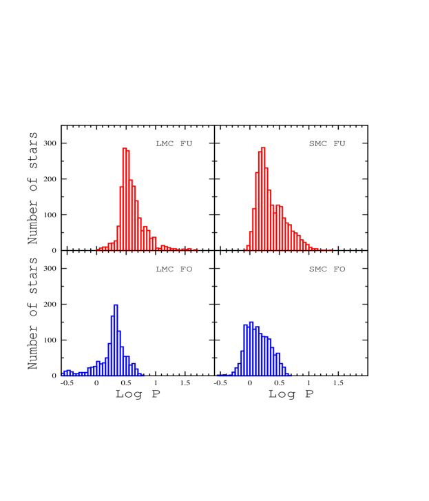
Figure 1: Period distributions for FU (top) and FO (bottom) LMC (left) and SMC (right) Cepheids.

3 Evolutionary and pulsation properties of MC Cepheids

The period distributions of FU (top) and FO (bottom) LMC and SMC Cepheids plotted in Fig. 1 show two well-known differences:

1. The peak in the period distribution of FU and FO SMC Cepheids is found at shorter periods compared with LMC Cepheids. In the former system, the peak is located at $\log P\sim$ 0.2 (FU) and $\sim$ 0.0 [days], while in the LMC, the peak is found at $\log P\sim$ 0.5 (FU) and $\sim$ 0.3 [days].

2. The period distribution of SMC Cepheids is broader than that of LMC Cepheids, and indeed in the former system the long-period tails of both the FU and FO Cepheids exhibit shallower profiles.

The intrinsic difference in the period distribution between LMC and SMC Cepheids, combined with the evidence that SMC Cepheids are, for a given period, systematically bluer than LMC and Galactic Cepheids, was noted more than 40 years ago by [Gascoigne (1969), Gascoigne (1974), Gascoigne (1969, 1974)]. On the basis of evolutionary and pulsation models, [Iben (1967), Iben (1967)] and [Christy (1971), Christy (1971)] suggested that these differences could be explained as a difference in metal content. The observational scenario was soundly confirmed by microlensing experiments ([Sasselov et al. (1997), Sasselov et al. 1997]; [Soszyński et al.(2012), Soszyński et al. 2012]) and more detailed theoretical investigations ([Bono et al. (2000), Bono et al. 2000]). The Cepheid period distribution might play a crucial role in constraining the recent star-formation rate and the properties of young stellar populations ([Alcock et al. (1999), Alcock et al. 1999]). However, the problem is far from trivial, since the period distribution depends not only on the initial mass function and the most recent star-formation episodes, but also on the Cepheid metallicity distribution.

Our knowledge of the metallicity distribution of MC Cepheids is quite limited. Accurate spectroscopic measurements based on high-resolution spectra are only available for a few dozen relatively bright Cepheids ([Luck et al. (1998), Luck et al. 1998]). On the basis of 22 LMC and 14 SMC Cepheids, [Romaniello et al. (2008), Romaniello et al. (2008)] found mean iron abundances for LMC Cepheids of [Fe/H] = $-0.33$ dex, with individual abundances ranging from $-0.62$ to 0.10 dex, while for SMC Cepheids [Fe/H] = $-0.75$ dex on average, with abundances ranging from $-0.87$ to $-0.63$ dex.

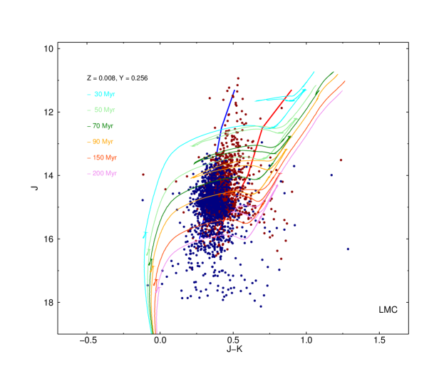
Figure 2: NIR ($J,J-K$) CMD of the FU (red) and FO (blue) LMC Cepheids. The differently colored lines display stellar isochrones with ages ranging from 30 to 200 Myr (see labels). The isochrones are based on non-canonical evolutionary models that include mild convective core overshooting during the central hydrogen-burning phase and a canonical mass-loss rate ($\eta=0.4$; [Pietrinferni et al. (2006), Pietrinferni et al. 2006]). They were constructed by assuming a scaled-solar chemical mixture at fixed metal ($Z=0.008$) and helium ($Y=0.256$) abundances. The vertical red and blue lines show the cool and hot edges, respectively, of the instability strip predicted by pulsation models. They account for the modal stability of both FU and FO Cepheids and have been constructed by assuming a non-canonical mass–luminosity relation and a similar chemical composition ([Marconi et al. (2005), Marconi et al. 2005]). Theoretical predictions were plotted by assuming a true distance modulus of $\mu=18.48$ mag a mean reddening of $E(V-I)=0.09$ mag ([Haschke et al.(2011), Haschke et al. 2011]) based on the reddening law of [Cardelli et al.(1989), Cardelli et al. (1989)].

To further constrain the evolutionary status of MC Cepheids, Fig. 2 shows the NIR ($J,J-K$) color–magnitude diagram (CMD) of the selected Cepheids. Data points plotted in Fig. 2 show that FO Cepheids (blue circles) attain, as expected, bluer colors compared with FU Cepheids (red circles). The colored lines show a set of isochrones with a scaled-solar chemical mixture and a chemical composition ($Z=0.008,Y=0.256$) typical of LMC Cepheids ([Pietrinferni et al. (2004), Pietrinferni et al. (2006), Pietrinferni et al. 2004, 2006]).The isochrones are based on evolutionary models that account for mild convective core overshooting during the central hydrogen-burning phase and include a canonical mass-loss rate ($\eta=0.4$). The comparison between theory and observations indicates that LMC Cepheids have ages ranging from a few tens to a couple of hundred Myr. The isochrones in the old ($t\approx 200$ Myr) and the young ($t\approx 30$ Myr) age ranges are characterized by ‘blue loops’ that do not cover the range in color of observed Cepheids. This is a well-known problem of intermediate-mass evolutionary models. The extent in color of the blue loops is affected by several physical mechanisms and by the input physics adopted. The treatment of mixing processes at the edge of the convective core and at the base of the convective envelope [Cassisi & Salaris (2011), (Cassisi & Salaris 2011)], as well as the mass-loss efficiency ([Matthews et al. (2012, Matthews et al. 2012]), are most popularly considered the culprits. However, the interested reader is referred to [Bono et al. (2000), Bono et al. (2000)], [Prada Moroni et al. (2012), Prada Moroni et al. (2012)], and [Neilson et al. (2011), Neilson et al. (2011)] for more detailed discussions.

The vertical blue and red lines show the predicted edges of the instability strip for a similar chemical composition. The blue and red lines account for the modal stability of both FU and FO Cepheids ([Marconi et al. (2005), Marconi et al. 2005]). Data points included in this figure reveal that theory and observations agree quite well. The predicted blue edge of the instability strip appears to be slightly cooler than the observed edge. However, the comparison between theory and observations was performed for fixed chemical composition, assuming the same reddening and neglecting depth effects. Cepheids located at fainter magnitudes and outside the instability strip are typically affected by higher extinction.

The SMC Cepheids show a very similar distribution in the NIR CMD (see Bono et al. 2000, their fig. 1). The difference in the period distribution between LMC and SMC Cepheids is explained by the current evolutionary framework. More metal-poor isochrones are characterized, at fixed age, by more extended blue loops. This means that the minimum mass crossing the instability strip decreases when moving from metal-rich to more metal-poor stellar systems. This difference, combined with the fact that the lifetime spent inside the instability strip by low-mass Cepheids is longer than for higher masses, causes an increase in the relative number of short-period Cepheids.

4 NIR PW relations

On the basis of two magnitudes (e.g., $m_{I}$ and $m_{V}$), we can define a Wesenheit index, e.g., $W(V,I)=m_{I}-[A_{I}/E(V-I)]\times(m_{V}-m_{I})$. We already mentioned that one of the main advantages of using PW relations for estimating Cepheid distances is that Wesenheit indices are independent of uncertainties affecting reddening estimates of Galactic and extragalactic Cepheids. Once we adopt a reddening law, the ratio of visual-to-selective absorption—$R_{V}=A_{V}/E(B-V)$—and assuming that the reddening law is universal, we can determine the color coefficient to define the Wesenheit pseudo-magnitudes.

The main advantage of using NIR measurements of Cepheids, compared with the use of optical data, is that their pulsation amplitude decreases with increasing wavelength. Therefore, estimating Cepheid mean magnitudes in NIR bands is easier than in optical bands. For the same reasons, the NIR bands are not well-suited for identification of classical Cepheids. Moreover, empirical and theoretical investigations indicate that NIR and optical–NIR PW relations are independent of metal abundance ([Bono et al. (2010), Bono et al. 2010]; [Majaess et al. (2011), Majaess et al. 2011]; [Inno et al, (2013), Inno et al. 2013]). To fully exploit these advantages, we performed a detailed and accurate analysis of NIR and optical–NIR PW relations (see Table 1).

Table 1: NIR and optical–NIR PW relations for LMC and SMC FU Cepheids.

$W(\lambda_{2},\lambda_{1})$1	$N_{c}$	$a$	$b$	$\sigma$2	$\mu$3 (mag)
LMC
$W(J,K_{\rm s})$	1708	15.876 $\pm$ 0.005	$-$3.365 $\pm$ 0.008	0.08	18.48 $\pm$ 0.02
$W(J,H)$	1701	15.630 $\pm$ 0.006	$-$3.373 $\pm$ 0.008	0.08	18.47 $\pm$ 0.02
$W(H,K_{\rm s})$	1709	16.058 $\pm$ 0.006	$-$3.360 $\pm$ 0.010	0.10	18.50 $\pm$ 0.02
$W(V,K_{\rm s})$	1737	15.901 $\pm$ 0.005	$-$3.326 $\pm$ 0.008	0.07	18.49 $\pm$ 0.02
$W(V,H)$	1730	15.816 $\pm$ 0.005	$-$3.315 $\pm$ 0.008	0.07	18.47 $\pm$ 0.02
$W(V,J)$	1732	15.978 $\pm$ 0.006	$-$3.272 $\pm$ 0.009	0.08	18.47 $\pm$ 0.02
$W(I,K_{\rm s})$	1737	15.902 $\pm$ 0.005	$-$3.325 $\pm$ 0.008	0.07	18.48 $\pm$ 0.02
$W(I,H)$	1734	15.801 $\pm$ 0.005	$-$3.317 $\pm$ 0.008	0.08	18.46 $\pm$ 0.02
$W(I,J)$	1735	16.002 $\pm$ 0.007	$-$3.243 $\pm$ 0.011	0.10	18.44 $\pm$ 0.02
$W(V,I)$	1700	15.899 $\pm$ 0.005	$-$3.327 $\pm$ 0.008	0.07	18.54 $\pm$ 0.02
Mean4					18.48 $\pm$ 0.01
SMC
$W(J,K_{\rm s})$	2448	16.457 $\pm$ 0.006	$-$3.480 $\pm$ 0.011	0.16	18.95 $\pm$ 0.02
$W(J,H)$	2448	16.217 $\pm$ 0.006	$-$3.542 $\pm$ 0.011	0.17	18.88 $\pm$ 0.02
$W(H,K_{\rm s})$	2448	16.457 $\pm$ 0.006	$-$3.480 $\pm$ 0.011	0.19	18.99 $\pm$ 0.02
$W(V,K_{\rm s})$	2295	16.507 $\pm$ 0.005	$-$3.461 $\pm$ 0.011	0.15	18.95 $\pm$ 0.02
$W(V,H)$	2285	16.426 $\pm$ 0.005	$-$3.475 $\pm$ 0.010	0.15	18.91 $\pm$ 0.02
$W(V,J)$	2286	16.614 $\pm$ 0.005	$-$3.427 $\pm$ 0.011	0.16	18.94 $\pm$ 0.02
$W(I,K_{\rm s})$	2294	16.511 $\pm$ 0.005	$-$3.464 $\pm$ 0.011	0.16	18.94 $\pm$ 0.02
$W(I,H)$	2202	16.417 $\pm$ 0.005	$-$3.480 $\pm$ 0.011	0.15	18.90 $\pm$ 0.02
$W(I,J)$	2279	16.662 $\pm$ 0.006	$-$3.424 $\pm$ 0.013	0.18	18.91 $\pm$ 0.02
$W(V,I)$	2260	16.482 $\pm$ 0.005	$-$3.449 $\pm$ 0.010	0.13	18.99 $\pm$ 0.02
Mean4					18.94 $\pm$ 0.01

Notes:
¹The color coefficients of the adopted PW relations are $\frac{A_{K}}{E(J-K_{\rm s})}=0.69$, $\frac{A_{H}}{E(J-H)}=1.63$, $\frac{A_{K}}{E(H-K_{\rm s})}=1.92$, $\frac{A_{K}}{E(V-K_{\rm s})}=0.13$, $\frac{A_{H}}{E(V-H)}=0.22$, $\frac{A_{J}}{E(V-J)}=0.41$, $\frac{A_{K}}{E(I-K_{\rm s})}=0.24$, $\frac{A_{H}}{E(I-H)}=0.42$, $\frac{A_{J}}{E(I-J)}=0.92$, and $\frac{A_{I}}{E(I-V)}=1.55$.
²Standard deviation of the linear fit (mag).
³Distance modulus based on the zero-point calibration of S11a.
⁴Weighted distance modulus estimated using the distance moduli of individual PW relations.

The results bearing on the linearity of the PW relations deserve a more detailed discussion. The evidence that optical and NIR PL relations might not be linear over the entire period range does not imply that NIR and optical–NIR PW relations have to show the same trend. The explanation is threefold.

1. [Bono & Marconi(1999), Bono & Marconi (1999)] suggested that PW relations mimic PLC relations. PLC relations, at fixed chemical composition, are intrinsically linear, because we correlate the pulsation period with both magnitude and color.

2. We can divide the sample into short- ($\log P\lesssim 0.4$ [days]) and long-period Cepheids, and provide new PW relations for the two different subsamples. The use of short- and long-period PW relations yields relative MC distances that are less accurate than relative distances based on PW relations covering the entire period range (Inno et al. 2012).

3. The zero points and slopes of the PW and PLC relations are fixed by the most commonly used Cepheids. A glance at the period distributions in Fig. 1 shows that they mainly depend on Cepheids that are located across the main peaks. This is the reason why short-period PW relations agree quite well with the PW relations based on the entire sample. However, the errors in the coefficients of the former PW relations are larger than the errors affecting the latter ([Inno et al, (2013), Inno et al. 2013]).

These results relating to the distance to the MCs rely on two independent calibrations of the zero points. The empirical calibration relies on trigonometric parallaxes of nine Galactic Cepheids, measured using the Fine Guidance Sensor on board the Hubble Space Telescope (HST; [Benedict et al.(2007), Benedict et al. 2007]). The theoretical calibration relies on different sets of nonlinear, convective models computed by [Bono et al. (2010), Bono et al. (2010)] and [Marconi et al. (2010), Marconi et al. (2010)]. To further constrain the intrinsic accuracy of the zero point of the new PW relations, we performed a new empirical calibration of 57 Galactic Cepheids. The main advantage of this sample is that their absolute magnitudes were estimated using a new calibration of the IRSB method ([Gieren et al., (2005), Gieren et al. 2005]; [Fouqué et al. (2007), Fouqué et al. 2007]; [Groenewegen(2008), Groenewegen 2008]), i.e. a variant of the Baade–Wesselink method. Note that the $p$ factor adopted in this relation to transform the radial velocity into a pulsation velocity was fixed using the HST Cepheids. This means that the current calibration (see Table 1) is not independent of the calibration based on HST Cepheids. However, we are using a sample of Cepheids that is a factor of six larger than that composed of HST Cepheids and they cover a broader range in metal abundance.

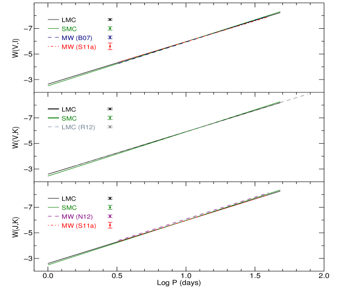
Figure 3: (top) Comparison of current PW $(V,I)$ relations for the LMC (black solid line) and SMC (green solid line), and similar PW relations for Galactic (MW) Cepheids provided by [Benedict et al.(2007), Benedict et al. (2007]; B07: dashed blue line) and [Storm et al. (2011a), Storm et al. (2011a]; S11a: dash-dotted red line). The different optical–NIR PW relations were plotted for the period range they cover. The vertical error bars display the dispersion of the different PW relations. (middle) Same as the top panel, but for the PW $(V,K_{\rm s})$ relations. The PW relation for the LMC was provided by [Ripepi et al. (2012), Ripepi et al. (2012]; R12: grey dashed line). (bottom) Same as the top panel, but for the PW $(J,K_{\rm s})$ relations. The PW $(J,K_{\rm s})$ relations for Galactic Cepheids by [Ngeow (2012), Ngeow (2012]; N12: purple) and S11a (red) are also plotted.

Fig. 3 shows a comparison between new NIR and optical–NIR relations for MC Cepheids and similar relations available in the literature. The MC and Galactic PW relations plotted in this figure agree quite well with each other. The difference in the zero points and slopes is smaller than the dispersion among the individual PW relations (see the error bars). Moreover, the new PW relations provide distances to the MCs that agree quite well with similar estimates available in the literature ([Inno et al, (2013), Inno et al. 2013]).

5 Conclusions and final remarks

New NIR measurements of MC Cepheids provide the opportunity to investigate the properties of both optical and NIR PW relations. Current results indicate that the PW relations are solid distance indicators, since the slopes, within $1\sigma$ errors, are independent of metal abundance. No firm conclusion can be reached regarding the zero points, since we still lack accurate parallaxes for metal-poor Cepheids. Trigonometric parallaxes are only available for a few nearby Galactic Cepheids ([Evans et al. (2005), Evans et al. 2005]; [Benedict et al.(2007), Benedict et al. 2007]).

The use of MC Cepheids in double-lined spectroscopic binaries appears a very promising and new, firm opportunity to overcome this long-standing problem (Pietrzyński et al. and Graczyk et al., this volume). These systems play a crucial role in constraining thorny systematic uncertainties affecting the Cepheid distance scale. They provide not only an independent absolute distance, but also a very precise measurement of their dynamical mass and radius ([Pietrzyński et al. (2010), Pietrzyński et al. (2011), Pietrzyński et al. 2010, 2011]). This information allows us to constrain the input physics adopted in evolutionary and pulsation models.

New optical and NIR surveys of nearby stellar systems provide a detailed census of regular variables, not only in dwarf irregulars ([Matsunaga et al. (2011), Matsunaga et al. 2011]; [Soszyński et al.(2012), Soszyński et al. 2012]), dwarf spheroidals ([pritzle, Pritzl et al. 2007]; [Fiorentino et al. (2012), Fiorentino et al. 2012]), dwarf spirals ([Scowcroft et al. (2009), Scowcroft et al. 2009]), and ultrafaint dwarfs ([Dall’Ora et al. (2012), Dall’Ora et al. 2012]), but also in M31 ([Fliri & Valls-Gabaud (2012), Fliri & Valls-Gabaud 2012]). The observational scenario as regards Galactic Cepheids has also been improved significantly, and indeed new NIR time-series data provide the opportunity to identify new Cepheids not only in the nuclear bulge, but also in the inner disk (Matsunaga, this volume). The NIR vvv survey will also provide a unique opportunity to discover new variables, and in particular Cepheids, along the Galactic plane ([Minniti et al. (2010), Minniti et al. 2010]). Despite these indisputable new results, we still lack detailed knowledge of the Cepheid distribution in the outer disk.

During the last 10 years, the number of Galactic Cepheids for which we have iron abundances based on spectroscopic measurements increased significantly. Thanks to the investigations by [Luck et al.(2011), Luck et al. (2011)], [Luck & Lambert (2011), Luck & Lambert (2011)], [Lemasle et al. (2007), Lemasle et al. (2008), Lemasle et al. (2007, 2008)], [Romaniello et al. (2008), Romaniello et al. (2008)], [Pedicelli et al. (2009), Pedicelli et al. (2009)], and K. Genovali et al. (in prep.), we have accurate iron abundances for $\sim$400 Galactic Cepheids.

We already mentioned that metallicity distributions of MC Cepheids only rely on a few dozen Cepheids. Spectroscopic surveys typically lag behind photometric surveys. However, the new massively multiplexed spectrograph (4MOST) for ESO’s 4m-class telescopes (VISTA, NTT) will certainly play a fundamental role in this context ([de Jong (2011), de Jong 2011]; [Ramsay et al. (2011), Ramsay et al. 2011]). This instrument will have a field of view in excess of 5 deg², more than 3000 fibers, and a spectral resolution ranging from 5000 to 20,000, offering a unique opportunity to map not only the MCs, but also nearby dwarfs and the Galactic plane. The same applies to MOONS, the optical and NIR spectrograph planned for the VLT ([cirascuolo11, Cirasuolo et al. 2011]), and to M2FS, the fiber-fed optical spectrograph at the Magellan II Clay telescope ([Mateo et al. (2012), Mateo et al. 2012]).

6 Acknowledgments

We are indebted to the editor, R. de Grijs, for his constant support. One of us (G.B.) thanks ESO for support as a science visitor. This work was partially supported by PRIN–INAF 2011, ‘Tracing the formation and evolution of the Galactic halo with VST’ (P.I. M. Marconi) and by PRIN–MIUR (2010LY5N2T) ‘Chemical and dynamical evolution of the Milky Way and Local Group galaxies’ (P.I.: F. Matteucci).

References

- [Alcock et al. (1999)] Alcock, C., Allsman, R.A., Alves, D.R., et al. 2000, AJ, 117, 920
- [Alcock et al. (2000)] Alcock, C., Allsman, R.A., Alves, D.R., et al. 2000, ApJ, 542, 281
- [Alibert et al. (1999)] Alibert, Y., Baraffe, I., Hauschildt, P., et al. 1999, A&A, 344, 551
- [Baade (1948)] Baade, W. 1948, PASP, 60, 230
- [Baraffe & Alibert] Baraffe, I., & Alibert, Y. 2001, A&A, 371, 592
- [Barnes & Evans (1976)] Barnes, T.G., & Evans, D.S. 1976, MNRAS, 174, 489
- [Becker et al. (1977)] Becker, S.A., Iben, I., Jr., & Tuggle, R.S. 1977, ApJ, 218, 633
- [Benedict et al.(2007)] Benedict, G.F., McArthur, B.E., Feast, M.W., et al. 2007, AJ, 133, 1810 (B07)
- [Bono & Marconi(1999)] Bono, G., & Marconi, M. 1999, in: New Views of the Magellanic Clouds (Chu, Y.-H., Suntzeff, N., Hesser, J., & Bohlender, D., eds), IAU Symp. Ser., 190, 527
- [Bono & Stellingwerf (1993)] Bono, G., & Stellingwerf, R.F. 1993, Mem. Soc. Astron. It., 64, 559
- [Bono et al. (2000)] Bono, G., Castellani, V., & Marconi, M. 2000, ApJ, 529, 293
- [Bono et al. (2010)] Bono, G., Caputo, F., Marconi, M., et al. 2010, ApJ, 715, 277
- [Buchler et al. (1990)] Buchler, J.R., Moskalik, P., & Kovacs, G. 1990, ApJ, 351, 617
- [Butler (1978)] Butler, C.J. 1978, A&AS, 32, 83
- [Caldwell & Coulson (1987)] Caldwell, J.A.R., & Coulson, I.M. 1987, AJ, 93, 1090
- [Cardelli et al.(1989)] Cardelli, J. A., Clayton, G. C., & Mathis, J. S. 1989, ApJ, 345, 245
- [Cassisi & Salaris (2011)] Cassisi, S., & Salaris, M. 2011, ApJ, 728, L43
- [Castor (1971)] Castor, J.I. 1971, ApJ, 166, 109
- [Christy (1968)] Christy, R.F. 1968, QJRAS, 9, 13
- [Christy (1971)] Christy, R.F. 1971, Astrophys. Space Sci. Libr., 23, 136
- [Christy (1975)] Christy, R.F. 1975, NASA Special Publ., 383, 85
- [Cirasuolo et al. (2011)] Cirasuolo, M., Afonso, J., Bender, R., et al. 2011, ESO Messenger, 145, 11
- [Cox (1979)] Cox, A.N. 1979, ApJ, 229, 212
- [Dall’Ora et al. (2012)] Dall’Ora, M., Kinemuchi, K., Ripepi, V., et al. 2012, ApJ, 752, 42
- [de Jong (2011)] de Jong, R. 2011, ESO Messenger, 145, 14
- [Evans et al. (2005)] Evans, N.R., Carpenter, K.G., Robinson, R., et al. 2005, AJ, 130, 789
- [Feast & Balona (1980)] Feast, M.W., & Balona, L.A. 1980, MNRAS, 192, 439
- [Fernie (1967)] Fernie, J.D. 1967, AJ, 72, 422
- [Fiorentino et al. (2012)] Fiorentino, G., Clementini, G., Marconi, M., et al. 2012, Ap&SS, 341, 143
- [Fliri & Valls-Gabaud (2012)] Fliri, J., & Valls-Gabaud, D. 2012, Ap&SS, 341, 57
- [Fouqué et al. (2007)] Fouqué, P., Arriagada, P., Storm, J., et al. 2007, A&A, 476, 73
- [Gascoigne & Kron (1965)] Gascoigne, S.C.B., & Kron, G.E. 1965, MNRAS, 130, 333
- [Gascoigne (1969)] Gascoigne, S.C.B. 1969, MNRAS146, 1
- [Gascoigne (1974)] Gascoigne, S.C.B. 1974, MNRAS166, 25
- [Gieren(1989)] Gieren, W.P. 1989, A&A, 225, 381
- [Gieren et al., (2005)] Gieren, W., Storm, J., Barnes, T.G., iii, et al. 2005, ApJ, 627, 224
- [Groenewegen(2004)] Groenewegen, M.A.T. 2004, MNRAS, 353, 903
- [Groenewegen(2008)] Groenewegen, M.A.T. 2008, A&A, 488, 25
- [Haschke et al.(2011)] Haschke, R., Grebel, E.K., & Duffau, S. 2011, AJ, 141, 158
- [Hubble (1953)] Hubble, E.P. 1953, MNRAS, 113, 658
- [Iben (1967)] Iben, I., Jr. 1967, ApJ, 147, 650
- [Iben (1974)] Iben, I., Jr. 1974, ARA&A, 12, 215
- [Iben & Tuggle (1975)] Iben, I., Jr., & Tuggle, R.S. 1975, ApJ, 197, 39
- [Inno et al, (2013)] Inno, L., Matsunaga, N., & Bono, G., et al. 2012, ApJ, in press, arXiv1212.4376
- [Kato et al. (2007)] Kato, D., Nagashima, C., Nagayama, T., et al. 2007, PASJ, 59, 615
- [Keller & Wood (2006)] Keller, S.C., & Wood, P.R. 2006 ApJ, 642, 834
- [Kippenhahn & Smith (1969)] Kippenhahn, R., & Smith, L. 1969, A&A, 1, 142
- [Kayser (1967)] Kayser, S.E. 1967, AJ, 72, 134
- [Kovtyukh et al. (2005)] Kovtyukh, V.V., Wallerstein, G., & Andrievsky, S.M. 2005, PASP, 117, 1173
- [Laney & Stobie (1986)] Laney, C.D., & Stobie, R.S. 1986, MNRAS, 222, 449
- [Laney & Stobie (1993)] Laney, C.D., & Stobie, R.S. 1993, MNRAS, 263, 921
- [Laney & Stobie (1994)] Laney, C.D., & Stobie, R.S. 1994, MNRAS, 266, 441
- [Lemasle et al. (2007)] Lemasle, B., François, P., Bono, G., et al. 2007, A&A, 467, 283
- [Lemasle et al. (2008)] Lemasle, B., François, P., Piersimoni, A., et al. 2008, A&A, 490, 613
- [Luck et al. (1998)] Luck, R.E., Moffett, T.J., Barnes, T.G., iii, et al. 1998, AJ, 115, 605
- [Luck et al.(2011)] Luck, R.E., Andrievsky, S.M., Kovtyukh, V.V., et al. 2011, AJ, 142, 51
- [Luck & Lambert (2011)] Luck, R.E., & Lambert, D.L. 2011, AJ, 142, 136
- [Macri et al. (2006)] Macri, L.M., Stanek, K.Z., Bersier, D., et al. 2006, ApJ, 652, 1133
- [Madore (1982)] Madore, B.F. 1982, ApJ, 253, 575
- [Majaess et al. (2011)] Majaess, D., Turner, D., & Gieren, W. 2011, ApJ, 741, L36
- [Marconi et al. (2005)] Marconi, M., Musella, I., & Fiorentino, G. 2005, ApJ, 632, 590
- [Marconi et al. (2010)] Marconi, M., Musella, I., Fiorentino, G., et al. 2010, ApJ, 713, 615
- [Marquette (1999)] Marquette, J.B. 1999, in: New Views of the Magellanic Clouds (Chu, Y.-H., Suntzeff, N., Hesser, J., & Bohlender, D., eds), IAU Symp. Ser., 190, 523
- [Mateo et al. (2012)] Mateo, M., Bailey, J.I., Crane, J., et al. 2012, Proc. SPIE, 8446, 84464Y
- [Matsunaga et al. (2011)] Matsunaga, N., Feast, M.W., & Soszyński, I. 2011, MNRAS, 413, 223
- [Matthews et al. (2012] Matthews, L.D., Marengo, M., Evans, N.R., & Bono, G. 2012, ApJ, 744, 53
- [Minniti et al. (2010)] Minniti, D., Lucas, P.W., Emerson, J.P., et al. 2010, New Astron., 15, 433
- [Neilson et al. (2011)] Neilson, H.R., Cantiello, M., & Langer, N. 2011, A&A, 529, L9
- [Ngeow et al. (2005)] Ngeow, C.-C., Kanbur, S.M., Nikolaev, S., et al. 2005, MNRAS, 363, 831
- [Ngeow & Kanbur (2008)] Ngeow, C.-C., & Kanbur, S.M. 2008, in: Galaxies in the Local Volume (Koribalski, B.S., & Jerjen, H., eds), p. 317
- [Ngeow (2012)] Ngeow, C.-C. 2012, ApJ, 747, 50 (N12)
- [Pedicelli et al. (2009)] Pedicelli, S., Bono, G., Lemasle, B., et al. 2009, A&A, 504, 81
- [Persson et al.(2004)] Persson, S.E., Madore, B.F., Krzemiński, W., et al. 2004, AJ, 128, 2239 (P04)
- [Pietrinferni et al. (2004)] Pietrinferni, A., Cassisi, S., Salaris, M., et al. 2004, ApJ, 612, 168
- [Pietrinferni et al. (2006)] Pietrinferni, A., Cassisi, S., Salaris, M., et al. 2006, ApJ, 642, 797
- [Pietrzyński et al. (2010)] Pietrzyński, G., Thompson, I.B., Gieren, W., et al. 2010, Nature, 468, 542
- [Pietrzyński et al. (2011)] Pietrzyński, G., Thompson, I.B., Graczyk, D., et al. 2011, ApJ, 742, L20
- [Pritzl et al. (2007)] Pritzl, B.J., Armandroff, T.E., Jacoby, G.H., & Da Costa, G.S. 2007, Bull. Am. Astron. Soc., 39, 845
- [Prada Moroni et al. (2012)] Prada Moroni, P.G., Gennaro, M., Bono, G., et al. 2012, ApJ, 749, 108
- [Ramsay et al. (2011)] Ramsay, S., Hammersley, P., & Pasquini, L. 2011, ESO Messenger, 145, 10
- [Ripepi et al. (2012)] Ripepi, V., Moretti, M.I., Marconi, M., et al. 2012, MNRAS, 424, 1807 (R12)
- [Romaniello et al. (2008)] Romaniello, M., Primas, F., Mottini, M., et al. 2008, A&A, 488, 731
- [Sakai et al. (2004)] Sakai, S., Ferrarese, L., Kennicutt, R.C., Jr., et al. 2004, ApJ, 608, 42
- [Sandage (1962)] Sandage, A. 1962, in: Problems of Extra-Galactic Research (McVittie, G.C., ed.), IAU Symp. Ser., 15, 359
- [Sandage & Tammann (1968)] Sandage, A., & Tammann, G.A. 1968, ApJ, 151, 531
- [Sandage & Tammann (1969)] Sandage, A., & Tammann, G.A. 1969, ApJ, 157, 683
- [Sandage et al. (2004)] Sandage, A., Tammann, G.A., & Reindl, B. 2004, A&A, 424, 43
- [Sasselov et al. (1997)] Sasselov, D.D., Beaulieu, J.P., Renault, C., et al. 1997, A&A, 324, 471
- [Scowcroft et al. (2009)] Scowcroft, V., Bersier, D., Mould, J.R., & Wood, P.R. 2009, MNRAS, 396, 1287
- [Soszyński et al.(2005)] Soszyński, I., Gieren, W., & Pietrzyński, G. 2005, PASP, 117, 823
- [Soszyński et al.(2012)] Soszyński, I., Udalski, A., Poleski, R., et al. 2012, Acta Astron., 62, 219
- [Stellingwerf (1982)] Stellingwerf, R.F. 1982, ApJ, 262, 339
- [Stellingwerf (1984)] Stellingwerf, R.F. 1984, ApJ, 284, 712
- [Stift (1982)] Stift, M.J. 1982, A&A, 112, 149
- [Stobie (1969)] Stobie, R.S. 1969, MNRAS, 144, 511
- [Storm et al. (2011a)] Storm, J., Gieren, W., Fouqué, P., et al. 2011a, A&A, 534, A94 (S11a)
- [Storm et al. (2011b)] Storm, J., Gieren, W., Fouqué, P., et al. 2011b, A&A, 534, A95 (S11b)
- [Welch (1994)] Welch, D.L. 1994, AJ, 108, 1421