The Fractional Ionization of the Warm Neutral Interstellar Medium

Abstract

When the neutral interstellar medium is exposed to EUV and soft X-ray radiation, the argon atoms in it are far more susceptible to being ionized than the hydrogen atoms. We make use of this fact to determine the level of ionization in the nearby, warm, neutral medium (WNM). By analyzing FUSE observations of ultraviolet spectra of 44 hot subdwarf stars a few hundred pc away from the Sun, we can compare column densities of Ar I to those of O I, where the relative ionization of oxygen can be used as a proxy for that of hydrogen. The measured deficiency $[{\rm Ar~{}I/O~{}I}]=-0.427\pm 0.11\,$dex below the expectation for a fully neutral medium implies that the electron density $n(e)\approx 0.04\,{\rm cm}^{-3}$ if $n({\rm H})=0.5\,{\rm cm}^{-3}$. This amount of ionization is considerably larger than what we expect from primary photoionizations resulting from cosmic rays, the diffuse X-ray background, and X-ray emitting sources within the medium, along with the additional ionizations caused by energetic secondary photoelectrons, Auger electrons, and photons from helium recombinations. We favor an explanation that bursts of radiation created by previous, nearby supernova remnants that have faded by now may have elevated the ionization, and the gas has not yet recombined to a quiescent level. A different alternative is that the low energy portion of the soft X-ray background is poorly shielded by the H I because it is frothy and has internal pockets of very hot, X-ray emitting gases.

1 INTRODUCTION

In large part, we are aware of the principal processes that create free electrons in otherwise completely neutral parts of the interstellar medium (ISM) in the disk of our Galaxy. However, for some of the contributing factors, ones that either enhance or diminish the relative ionization of the gas, there is a need to validate our understanding of their strengths. Most of these processes are well understood qualitatively, but one major quantitative uncertainty is the effectiveness of extreme ultraviolet (EUV) and soft X-ray photons in ionizing the gas. Two factors contribute to this uncertainty: one is the difficulty in measuring the fluxes of diffuse photons with energies above the ionization potential of hydrogen (13.6 eV) but below about 100 eV, and the other is an overall assessment of how well these photons can penetrate the neutral regions, which depends on the porosity of the gas structures and the distribution of radiation sources.

Our ultimate goal is not only to understand these processes better, but also to obtain an estimate for the fractional amount of the gas that is in an ionized state. This information is relevant to gauging the strength of heating of the gas due to the photoelectric effect from dust grains irradiated by starlight, since the grain charge, which regulates its rate, depends on the electron density (Weingartner & Draine 2001b). While generally considered to be less important than the photoelectric effect, other means of creating thermal energy, such as the heating caused by secondary electrons from cosmic ray and X-ray ionizations and the dissipation of Alfvén waves and magnetosonic turbulence (Kulsrud & Pearce 1969; McIvor 1977; Spangler 1991; Minter & Spangler 1997; Lerche et al. 2007), depend on the relative fractions of electrons. Cooling of the gas through the collisional excitation of the fine-structure levels of C⁺, Si⁺ and Fe⁺ or, at temperatures approaching $10^{4}\,$K various metastable levels and the L$\alpha$ transition of hydrogen, are likewise governed by the degree of partial ionization (Dalgarno & McCray 1972). In the following paragraphs, we consider three different pathways for creating small amounts of ionization in the mostly neutral ISM.

Except for the interiors of dense clouds where there is significant extinction, all of the space in the disk of our Galaxy is exposed to ultraviolet starlight photons that are capable of ionizing atoms that have first ionization potentials less than that of hydrogen (13.6 eV). Since the recombination rates of the ions are slow relative to their ionization rates, the concentrations of the ionized states of these atoms are strongly dominant. Thus, it is a simple matter to add together the contributions from various elements that are able to supply free electrons. The only uncertainty here is an accounting of the strengths of depletions from the gas phase caused by these elements condensing into solid form onto dust grains. These strengths vary collectively for all of the elements from one region to the next. If we take such variations into account (Jenkins 2009), we can state that most of the gas will have free electron contributions that should be somewhere in the range $n({\rm M}^{+})=0.8-1.7\times 10^{-4}n({\rm H}_{\rm tot})$, where $n({\rm M}^{+})$ is the number density of heavy elements that are capable of being ionized and $n({\rm H}_{\rm tot})$ is the total density of hydrogen in both neutral and ionized forms.

As cosmic ray particles collide with gas atoms in the Galaxy, they heat and ionize the ISM. We are unable to observe the flux of the lowest energy particles because we are shielded from them by the heliospheric magnetic field, and extrapolations from the observed higher energy flux distributions are uncertain (Spitzer & Tomasko 1968). Nevertheless, from measurements of the relative abundances of trace molecular species, the cosmic ray ionization rates $\zeta_{\rm CR}\approx 0.5-9\times 10^{-16}{\rm s}^{-1}$ seems to be the most plausible range for the general ISM (Wagenblast & Williams 1996; Liszt 2003; Indriolo et al. 2007; Neufeld et al. 2010; Indriolo & McCall 2012), although details in the chemical models may introduce some uncertainty [cf. Le Petit et al. (2004) and Shaw et al. (2008)]. The chemical models of Bayet et al. (2011) suggest that in some particularly active regions the ionization rates may increase to $\zeta_{\rm CR}>1\times 10^{-14}{\rm s}^{-1}$.

We now consider a third mechanism for ionizing the gas, one that is harder to quantify than the other two. EUV and soft X-ray radiation can ionize atoms, through both the action of primary photoionizations and by creating a cascade of energetic, secondary photoelectrons that can collisionally ionize other atoms. Estimates of the effectiveness of these agents are difficult to synthesize, since there are many complicating factors. At high energies, much of the radiation arises from cooling, very hot ($T>10^{6}\,$K) gas coming from recently shocked regions within the disk and halo of our Galaxy. For energies slightly above about 100 eV, the photons can survive a journey through the neutral medium up to about $N({\rm H}^{0})=2\times 10^{19}\,{\rm cm}^{-2}$, and this penetration depth progressively increases with energy. Supplementing this ionizing radiation is that coming from several kinds of sources that are embedded within the neutral medium. These include stars over a wide range of spectral types on the main sequence, active X-ray binaries, and the plentiful, but faint white dwarf (WD) stars.

2 STRATEGY OF THE INVESTIGATION

The objective of the current study is to use specialized observations to help resolve the uncertainties that were mentioned above and gain a quantitative insight on how effectively the neutral regions are partially photoionized by EUV and X-ray radiation. We do this by repeating a method developed by Sofia & Jenkins (1998, hereafter SJ98), who examined interstellar UV absorption features that could be seen in the spectra of background stars so that they could compare the abundance of the neutral form of argon, which is highly susceptible to being photoionized, to that of hydrogen, which has an ionization potential very close to that of argon but with a markedly lower ionization cross section. We propose that it is safe to assume that the abundance of argon (both neutral and ionized) relative to that of hydrogen should be equal to the solar ratio. For instance, SJ98 presented arguments that support the principle that argon in the gas phase is not likely to be depleted by being incorporated into an atomic matrix within interstellar dust grains. We will reinforce this idea with some indirect observational evidence in Section 4.2.1. Thus, we operate on the principle that any deficiency of neutral argon (Ar I) below our expectation for the amount of H I that is present may be considered to arise from the conversion of Ar to its ionized form, which is invisible.

The investigation by SJ98 covered an extremely limited number of target stars observed with the Interstellar Medium Absorption Profile Spectrograph (IMAPS) (Jenkins et al. 1996). Later, Jenkins et al. (2000b) and Lehner et al. (2003) reported on observations of absorption features of Ar I observed by the Far Ultraviolet Spectroscopic Explorer (FUSE) (Moos et al. 2000; Sahnow et al. 2000) toward collections of WD stars inside and slightly beyond the edge of the Local Bubble, in order to infer ionization conditions of clouds subjected to the characteristic radiation field in our immediate neighborhood. Our current goal is to extend our reach well beyond the stars surveyed in these two studies, again by using FUSE spectra, so that we can sample regions of more typical densities well outside the Local Bubble. We do this by downloading from the Mikulski Archive for Space Telescopes (MAST) at the Space Telescope Science Institute a large collection of FUSE spectra of hot subdwarf stars that are situated several hundred pc away from us, well beyond the boundary of the Local Bubble.

Our ultimate objective is to compare the neutral fractions of Ar and H, as had been done in past investigations. However, a conventional approach of simply deriving the two column densities and dividing one by the other is not easily achievable with the data in this survey for two reasons. First, it is difficult to measure $N$(Ar I) because the lines are saturated, but only moderately so, and recorded at low resolution. Second, the amount of H I on a sight line can usually be determined from the damping wings of L$\alpha$, but when the interstellar column density is low and there is a significant stellar L$\alpha$ absorption, one must know the star’s effective temperature and surface gravity and then create a model for the stellar feature, against which the interstellar feature is superimposed. Also, as emphasized by Sofia et al. (2011) measurements of $N$(H I) using the damping wings of L$\alpha$ can give a misleading outcome if one does not know about and correct for the effects of the velocity structures of the gas. This problem is probably most severe for low column density cases in the present study.

We can overcome the difficulties mentioned above if we replace H with O as the comparison element. In the wavelength coverage of FUSE there are a large number of O I absorption features, and these lines cover a broad range of transition probabilities. Most important, the strengths of the O I features are comparable to the one available feature of Ar I. By a simple comparison of the strength of this Ar I line to those of O I, we can determine $N({\rm Ar~{}I})/N({\rm O~{}I})$. We describe this process in more detail in Section 4.2.

The ionization fraction of O is strongly locked to that of H through a strong charge exchange reaction (Field & Steigman 1971; Chambaud et al. 1980; Stancil et al. 1999). Thus we can use O as a proxy for H. The only shortcoming of this tactic is that O can be depleted in the ISM, but the depletion factors are not very large in the regimes of low densities considered here (Cartledge et al. 2004, 2008; Jenkins 2009).

Section 3 of this paper describes the selection of archival FUSE spectra and how they were processed to yield useful presentations of the absorption features for measurements of equivalent widths. Our method of interpreting the spectra to yield the ionization of Ar relative to that of O is presented in Section 4. Section 5 contains a short digression on how we verify that the target stars are beyond the edge of the Local Bubble. In Section 6 we outline the basic equations that take into account the processes that influence the partial ionizations of Ar, relative to those of H and O. The equations presented in this section are virtually identical to those outlined by SJ98, but with some new refinements (i.e., a few reactions that were not included earlier). We consider the creation of free electrons from the starlight ionization of heavy elements and the effects from cosmic rays as processes that are mostly understood and already accounted for, and view the actions arising from EUV and X-ray ionizations as the principal unknowns whose strengths are to be determined. In Section 7 we make a prediction for the degree of ionization produced by known sources of radiation, but find that in order to satisfy the general outcomes for our measured ratios of Ar I to O I, an extraordinarily low volume density of hydrogen $n({\rm H}_{\rm tot})$ is required. In order to obtain the same results for higher densities, we must propose a means of achieving higher levels of ionization. In Section 8 we propose two possibilities: (1) there is a large residual ionization left over from effects of radiation emitted by nearby, but now extinct supernova remnants (SNRs) over the past several Myr or (2) the neutral medium is porous enough to allow external, low-energy photons to penetrate the gas with less than the expected amount of attenuation. Section 9 presents an overview of the implications of our results on an assortment of physical processes and various other kinds of observations that depend on electron fractions in the diffuse, neutral medium. The paper ends with a summary of the main conclusions (Section 10).

Appendices to this paper give descriptions of various atomic processes that were incorporated into the calculations, but at a level of detail that most readers may wish to ignore. A general section on the ionizations arising from secondary electrons (Appendix A) is broken into two subsections: one treats the effects from electrons liberated by the ionizations of H and He (Section A.1), while the second one discusses primary and Auger electrons created by the inner shell X-ray ionizations of heavy elements (Section A.2). Appendix B gives the equations for evaluating the effects from a multitude of different kinds of ionizing photons that arise from the recombination of He⁺⁺ and He⁺ ions with free electrons. Finally, Appendix C describes how we can estimate the rates of cosmic ray ionization of H⁰, He⁰ and Ar⁰ from the observed rates that apply to molecular hydrogen in dense clouds.

3 OBSERVATIONS

3.1 Target Selection

Our objective was to make use of target stars that represented intermediate cases between nearby WD stars, whose sight lines are entirely or heavily influenced by conditions in the Local Bubble, and the much more distant hot main-sequence, giant or supergiant stars that can create their own enhanced ionizations in atypical concentrations of gas associated with their formation. Hot subdwarf stars represent a class of objects that fall into this intermediate category. They have distances that are of order a few hundred parsecs from us, which reduces the contribution from material in the Local Bubble to a very minor level. Since they are old, they have had adequate time to escape from their progenitorial gas clouds, and thus their locations are essentially random and should show no preference for dense gas complexes. They have the additional advantage that they are bright enough to yield good quality spectra, but they are not so bright that they exceed the maximum allowed count-rate levels for FUSE.

In an initial screening of prospective targets, we examined the quick-look plots of all stars classified as sdO and sdB spectral types in the MAST archive of FUSE data. In this step, we rejected all spectra that either seemed to show very strong stellar spectral features (8 stars) or that had an inadequate signal-to-noise ratio ($S/N$) at wavelengths in the vicinity of 920 Å (70 stars), which is where most of the O I lines are situated. A few further rejections were made after the spectra were downloaded and found to have observing anomalies (an extraordinarily large number of missing observations caused by channel misalignments: 3 stars), strong stellar features that were not evident in the quick-look plots (3 stars), or molecular hydrogen lines that were strong enough to seriously compromise the lines that we wanted to measure (2 stars). The lack of stars with exceptionally strong H₂ features helped to eliminate sight lines that penetrate dense, cool gas clouds.

3.2 Creation of the Spectra

All of the downloads of the calibrated FUSE data from MAST occurred well after the final pipeline reductions were performed for the archive with CalFUSE version 3.2.3 (Dixon et al. 2007). For every target, we accepted data from all of the available observing sessions (identified by unique archive root names) but rejected any subexposures that had an extraordinarily low count level caused by a channel misalignment during the observation. We used exposures obtained during both orbital day and night. Normally, one must be cautious about observations of features for either O I or N I because they can be filled in by diffuse telluric emission lines during daytime observing. However the O I transition strengths considered here are so weak that the telluric contributions are insignificant.

All subexposures and spectral channels that passed our initial screening were coadded with weight factors based on the inverse squares of their respective values of $S/N$ for intensities smoothed over a wavelength interval of 0.12 Å (or 9 independent spectral elements – this ensures that weights are not strongly influenced by random noise excursions). Before this coaddition took place, we examined some strong interstellar features and aligned the individual spectra in wavelength against a preliminary coaddition with no wavelength shifts. This process enabled us to virtually eliminate any degradation in resolution caused by drifts of the spectra in the wavelength direction from one subexposure to the next. However, there can still be overall small systematic errors in radial velocity of about $10\,{\rm km~{}s}^{-1}$; see Appendix A of Bowen et al. (2008). In a few cases, the spectral $S/N$ values were too low to allow such shifts to be made with much confidence, even after the intensities were smoothed with a median filter for viewing. Such spectra were combined without any shifts. For every target, two combined spectra were created: one was made up with shifts appropriate to the spectral region covering the Ar I line at 1048 Å, while the other had differentials that were optimized for the wavelengths that covered the weakest O I lines near 920 Å.

4 ANALYSIS

4.1 Equivalent Widths and Their Errors

We measured equivalent widths of the Ar I and O I lines by integrating intensity deficits below best-fitting Legendre polynomials for the continua defined from intensities at locations somewhat removed from the features. Special precautions were made to account for various sources of error, which are important for later analysis stages that assign relative weights to different measurements and also for the estimates of the ultimate errors in the results. First, we accounted for the direct effect that random count-rate variations can have on the equivalent width outcome (Jenkins et al. 1973). Next, the weakest lines are subject to uncertainties arising from improper definitions of the continua. To construct the probable errors, we evaluated the expected formal errors in the polynomial coefficients, as described by Sembach & Savage (1992), and then we multiplied them by 2 in order to make an approximate allowance for additional uncertainties caused by the arbitrariness in selecting the most appropriate polynomial order. To find the effects of these continuum errors on our measurements, the equivalent widths were re-evaluated using the probable excursions of the continua on either side of the preferred ones. Errors in the background subtraction in the FUSE data processing are small compared to the other errors.

Table 1: Equivalent Widths

	Ar I	O I
	1048.220	919.917	922.200	925.446	916.815	930.257	919.658	921.857	924.950	950.885	976.448	948.686	971.738
Star Name	2.440	$-0.788$	$-0.645$	$-0.484$	$-0.362$	$-0.301$	$-0.137$	$-0.001$	0.155	0.176	0.509	0.778	1.052
	$\cdots$	11.6	15.3	20.6	25.0	27.8	34.5	40.4	46.9	49.0	$\cdots$	$\cdots$	$\cdots$
(1)	(2)	(3)	(4)	(5)	(6)	(7)	(8)	(9)	(10)	(11)	(12)	(13)	(14)
2MASS15265306
+7941307	$77\pm 18$	$(14\pm 16)$	$(-4\pm 16)$	$29\pm 12$	$\cdots$	$24\pm 22$	$41\pm 22$	$39\pm 19$	$84\pm 11$	$59\pm 15$	$97\pm 12$	$111\pm 11$	$(120\pm 12)$
AA Dor	$60\pm 10$	$30\pm 18$	$\cdots$	$56\pm 13$	$\cdots$	$75\pm 31$	$51\pm 37$	$\cdots$	$93\pm 13$	$73\pm 21$	$(121\pm 19)$	$\cdots$	$(225\pm 9)$
AGK+81 266	$76\pm 19$	$22\pm 15$	$44\pm 15$	$33\pm 15$	$\cdots$	$60\pm 19$	$76\pm 15$	$87\pm 18$	$99\pm 14$	$122\pm 14$	$(116\pm 18)$	$(102\pm 15)$	$(125\pm 14)$
BD+18 2647	$43\pm 18$	$22\pm 13$	$\cdots$	$37\pm 11$	$\cdots$	$26\pm 16$	$39\pm 18$	$\cdots$	$78\pm 11$	$68\pm 11$	$(63\pm 13)$	$(131\pm 12)$	$(159\pm 11)$
BD+25 4655	$33\pm 18$	$3\pm 12$	$\cdots$	$18\pm 12$	$\cdots$	$22\pm 11$	$21\pm 12$	$\cdots$	$53\pm 11$	$41\pm 12$	$64\pm 13$	$77\pm 12$	$(75\pm 11)$
BD+28 4211	$31\pm 8$	$14\pm 3$	$27\pm 5$	$24\pm 3$	$25\pm 4$	$37\pm 4$	$34\pm 4$	$35\pm 4$	$42\pm 3$	$51\pm 3$	$(42\pm 4)$	$(83\pm 4)$	$(62\pm 3)$
BD+37 442	$166\pm 7$	$\cdots$	$61\pm 28$	$107\pm 16$	$\cdots$	$95\pm 24$	$\cdots$	$166\pm 17$	$128\pm 16$	$\cdots$	$\cdots$	$\cdots$	$\cdots$
BD+39 3226	$54\pm 3$	$(21\pm 8)$	$(81\pm 8)$	$34\pm 7$	$40\pm 8$	$48\pm 10$	$47\pm 8$	$38\pm 8$	$52\pm 7$	$59\pm 7$	$54\pm 7$	$69\pm 8$	$(73\pm 7)$
CPD$-$31 1701	$16\pm 8$	$11\pm 5$	$\cdots$	$19\pm 4$	$\cdots$	$20\pm 11$	$39\pm 6$	$\cdots$	$45\pm 4$	$(28\pm 5)$	$(45\pm 7)$	$(68\pm 5)$	$(91\pm 4)$
CPD$-$71D172	$34\pm 10$	$31\pm 13$	$34\pm 13$	$52\pm 12$	$\cdots$	$57\pm 13$	$47\pm 15$	$36\pm 18$	$67\pm 12$	$67\pm 13$	$(61\pm 13)$	$(93\pm 13)$	$(83\pm 14)$
EC11481$-$2303	$132\pm 16$	$(39\pm 17)$	$\cdots$	$75\pm 16$	$\cdots$	$92\pm 16$	$99\pm 17$	$80\pm 34$	$145\pm 15$	$121\pm 17$	$153\pm 17$	$146\pm 16$	$177\pm 16$
Feige 34	$36\pm 17$	$(9\pm 13)$	$\cdots$	$13\pm 13$	$\cdots$	$28\pm 14$	$38\pm 13$	$\cdots$	$42\pm 13$	$46\pm 14$	$41\pm 21$	$86\pm 19$	$\cdots$
HD 113001	$115\pm 20$	$(28\pm 10)$	$\cdots$	$(50\pm 10)$	$\cdots$	$(53\pm 15)$	$63\pm 10$	$\cdots$	$96\pm 10$	$93\pm 12$	$100\pm 13$	$125\pm 11$	$128\pm 10$
JL 119	$112\pm 5$	$52\pm 14$	$39\pm 27$	$89\pm 8$	$\cdots$	$103\pm 15$	$83\pm 25$	$80\pm 23$	$138\pm 7$	$111\pm 19$	$(169\pm 7)$	$(180\pm 6)$	$(174\pm 7)$
JL 25	$77\pm 19$	$29\pm 17$	$\cdots$	$43\pm 17$	$\cdots$	$72\pm 22$	$29\pm 17$	$\cdots$	$69\pm 17$	$94\pm 17$	$\cdots$	$111\pm 18$	$106\pm 17$
JL 9	$100\pm 10$	$46\pm 12$	$\cdots$	$67\pm 9$	$\cdots$	$95\pm 16$	$87\pm 14$	$\cdots$	$106\pm 9$	$116\pm 9$	$\cdots$	$129\pm 11$	$(142\pm 12)$
LB 1566	$57\pm 6$	$32\pm 13$	$\cdots$	$51\pm 11$	$\cdots$	$56\pm 14$	$48\pm 15$	$\cdots$	$81\pm 11$	$73\pm 19$	$(98\pm 11)$	$(108\pm 14)$	$(111\pm 11)$
LB 1766	$67\pm 16$	$-3\pm 13$	$\cdots$	$61\pm 12$	$\cdots$	$58\pm 14$	$38\pm 14$	$\cdots$	$98\pm 11$	$\cdots$	$120\pm 11$	$(148\pm 10)$	$(168\pm 10)$
LB 3241	$56\pm 9$	$29\pm 8$	$25\pm 9$	$54\pm 8$	$\cdots$	$53\pm 8$	$52\pm 8$	$97\pm 8$	$82\pm 7$	$106\pm 7$	$(112\pm 7)$	$(123\pm 7)$	$(128\pm 7)$
LS 1275	$62\pm 15$	$29\pm 10$	$42\pm 12$	$45\pm 9$	$52\pm 14$	$65\pm 13$	$46\pm 10$	$(99\pm 13)$	$58\pm 9$	$74\pm 10$	$80\pm 10$	$89\pm 11$	$(89\pm 9)$
LSE 234	$115\pm 12$	$(47\pm 16)$	$72\pm 17$	$76\pm 15$	$\cdots$	$94\pm 16$	$85\pm 18$	$123\pm 17$	$107\pm 15$	$122\pm 15$	$\cdots$	$154\pm 18$	$130\pm 15$
LSE 259	$149\pm 6$	$\cdots$	$\cdots$	$88\pm 14$	$\cdots$	$134\pm 20$	$\cdots$	$\cdots$	$123\pm 13$	$156\pm 13$	$\cdots$	$\cdots$	$\cdots$
LSE 263	$119\pm 17$	$(49\pm 14)$	$\cdots$	$73\pm 12$	$101\pm 19$	$80\pm 15$	$76\pm 14$	$\cdots$	$91\pm 13$	$76\pm 13$	$95\pm 17$	$139\pm 14$	$159\pm 12$
LSE 44	$93\pm 12$	$56\pm 11$	$68\pm 12$	$68\pm 10$	$\cdots$	$78\pm 15$	$61\pm 15$	$94\pm 12$	$92\pm 9$	$132\pm 10$	$\cdots$	$(140\pm 10)$	$(107\pm 11)$
LSII+18 9	$91\pm 15$	$\cdots$	$\cdots$	$54\pm 21$	$66\pm 38$	$73\pm 23$	$72\pm 21$	$\cdots$	$78\pm 21$	$125\pm 21$	$\cdots$	$\cdots$	$(119\pm 21)$
LSII+22 21	$45\pm 12$	$27\pm 10$	$\cdots$	$35\pm 9$	$40\pm 15$	$52\pm 13$	$44\pm 11$	$(116\pm 8)$	$63\pm 8$	$74\pm 9$	$(91\pm 8)$	$(100\pm 9)$	$(119\pm 8)$
LSIV+10 9	$179\pm 12$	$(58\pm 10)$	$\cdots$	$88\pm 9$	$\cdots$	$106\pm 18$	$88\pm 12$	$\cdots$	$152\pm 9$	$170\pm 10$	$231\pm 9$	$\cdots$	$(192\pm 10)$
LSS 1362	$88\pm 3$	$(39\pm 11)$	$52\pm 14$	$59\pm 8$	$\cdots$	$78\pm 18$	$64\pm 20$	$(65\pm 8)$	$(68\pm 10)$	$134\pm 7$	$\cdots$	$\cdots$	$\cdots$
MCT 2005
$-$5112	$103\pm 8$	$\cdots$	$\cdots$	$74\pm 11$	$\cdots$	$75\pm 18$	$\cdots$	$\cdots$	$113\pm 9$	$135\pm 12$	$(168\pm 15)$	$(150\pm 13)$	$(124\pm 18)$
MCT 2048
$-$4504	$122\pm 12$	$\cdots$	$86\pm 21$	$83\pm 15$	$\cdots$	$61\pm 59$	$\cdots$	$90\pm 28$	$118\pm 14$	$117\pm 17$	$149\pm 14$	$174\pm 16$	$(172\pm 15)$
NGC6905
star	$147\pm 8$	$(45\pm 39)$	$\cdots$	$101\pm 39$	$\cdots$	$83\pm 43$	$62\pm 46$	$\cdots$	$139\pm 38$	$167\pm 38$	$205\pm 39$	$\cdots$	$(154\pm 39)$
PG0919+272	$55\pm 27$	$34\pm 17$	$31\pm 16$	$43\pm 16$	$45\pm 27$	$83\pm 17$	$59\pm 17$	$64\pm 16$	$81\pm 15$	$65\pm 17$	$87\pm 15$	$108\pm 16$	$(106\pm 15)$
PG0952+519	$52\pm 3$	$19\pm 8$	$\cdots$	$36\pm 7$	$\cdots$	$43\pm 8$	$53\pm 9$	$\cdots$	$74\pm 7$	$\cdots$	$(125\pm 6)$	$(154\pm 8)$	$(148\pm 6)$
PG1032+406	$-21\pm 27$	$3\pm 23$	$11\pm 19$	$15\pm 18$	$(95\pm 24)$	$20\pm 19$	$-2\pm 36$	$36\pm 18$	$15\pm 17$	$72\pm 17$	$46\pm 20$	$70\pm 18$	$(94\pm 17)$
PG1051+501	$165\pm 15$	$\cdots$	$\cdots$	$81\pm 30$	$\cdots$	$64\pm 33$	$\cdots$	$\cdots$	$128\pm 27$	$142\pm 28$	$\cdots$	$\cdots$	$185\pm 28$
PG1230+068	$102\pm 15$	$40\pm 8$	$45\pm 11$	$72\pm 7$	$\cdots$	$82\pm 16$	$86\pm 9$	$79\pm 13$	$110\pm 7$	$88\pm 8$	$105\pm 18$	$126\pm 7$	$(139\pm 7)$
PG1544+488	$84\pm 3$	$26\pm 11$	$25\pm 13$	$56\pm 8$	$76\pm 34$	$69\pm 10$	$74\pm 13$	$89\pm 11$	$91\pm 7$	$97\pm 9$	$(124\pm 11)$	$(132\pm 7)$	$(151\pm 8)$
PG1605+072	$131\pm 15$	$\cdots$	$\cdots$	$72\pm 21$	$\cdots$	$99\pm 25$	$\cdots$	$\cdots$	$136\pm 20$	$163\pm 20$	$229\pm 20$	$(166\pm 22)$	$(186\pm 20)$
PG1610+519	$122\pm 9$	$\cdots$	$\cdots$	$81\pm 12$	$\cdots$	$\cdots$	$\cdots$	$\cdots$	$150\pm 9$	$\cdots$	$256\pm 5$	$\cdots$	$(228\pm 7)$
PG2158+082	$117\pm 7$	$\cdots$	$\cdots$	$100\pm 19$	$\cdots$	$97\pm 26$	$\cdots$	$\cdots$	$121\pm 19$	$175\pm 17$	$\cdots$	$(154\pm 22)$	$\cdots$
PG2317+046	$68\pm 20$	$49\pm 18$	$29\pm 31$	$61\pm 19$	$\cdots$	$50\pm 24$	$28\pm 21$	$48\pm 33$	$71\pm 18$	$135\pm 18$	$\cdots$	$132\pm 19$	$(81\pm 19)$
Ton 102	$51\pm 13$	$21\pm 15$	$22\pm 16$	$26\pm 16$	$\cdots$	$39\pm 16$	$34\pm 16$	$79\pm 16$	$42\pm 17$	$63\pm 16$	$72\pm 15$	$\cdots$	$\cdots$
Ton S227	$80\pm 25$	$27\pm 10$	$26\pm 11$	$43\pm 10$	$\cdots$	$21\pm 20$	$27\pm 11$	$30\pm 12$	$58\pm 9$	$\cdots$	$85\pm 11$	$111\pm 12$	$121\pm 9$
UV0904$-$02	$69\pm 4$	$(30\pm 9)$	$\cdots$	$43\pm 8$	$\cdots$	$59\pm 12$	$52\pm 10$	$\cdots$	$67\pm 7$	$65\pm 11$	$75\pm 7$	$84\pm 8$	$(89\pm 7)$

The sources of error mentioned above are straightforward to evaluate and would apply to just about any measure of an equivalent width. However, with the subdwarf stars, we must also contend with the confusion produced by stellar lines. We made no attempt to model such features, because in order to do so we would need to know the details of the stellar parameters for each star. Instead, we regarded the influence of stellar features as random sources of error in our line measurements. In order to estimate the amplitude of such errors, which can vary markedly from one star to the next and can change with wavelength, we measured for each target the variance of a large number of equivalent width measurements of imaginary, fake lines at wavelengths similar to the ones under study, but that were displaced away from known real interstellar lines, both atomic and molecular. This variance was then used as a guide for estimating the errors that should arise from stellar features.

Figure 1 shows samples of spectra covering the relevant wavelength regions for two stars. These two cases illustrate strong differences in the degree of interference from stellar lines. The first example, AGK+81 266, has many stellar lines that can either add an apparent absorption to an interstellar line or distort the continuum level that is measured on either side of the line. For this target, these effects dominate over other sources of error and create $1\sigma$ uncertainties in $W_{\lambda}$ equal to 18.5 and 14.2 mÅ for the Ar I and O I lines, respectively. This star also exhibits molecular hydrogen features of moderate strength, but here the lines are not strong enough to compromise the measurements of the atomic lines. A far more favorable case for measuring interstellar features is presented by the star UV0904$-$02. Here, uncertainties produced by random stellar features should create errors of only 3.6 mÅ for the Ar I line and 6.6 mÅ for the O I lines.

All of the errors discussed in this section were combined in quadrature to synthesize the overall errors in the equivalent widths. Values for the equivalent widths of all lines and their associated uncertainties are listed for each of our targets in Table 1. The columns in this table are arranged in a sequence from the weakest to the strongest lines.

4.2 Derivations of [Ar I/O I] Values and Their Uncertainties

4.2.1 Reference Abundances

Detailed discussions on various methods of measuring the protosolar and B-star abundances of Ar have been presented by Lodders (2008) and Lanz et al. (2008). We adopt a mean value for the recommended outcomes of the two, $\log({\rm Ar/H})+12=6.60\pm 0.10$. (Since both determinations might be subject to common errors, the error of the mean is not reduced below the 0.10 dex errors specified by each of them.) This value is higher than the solar photospheric value proposed by Asplund et al. (2009), and it remains so even after one applies a correction for gravitational settling of $+0.07\,$dex (Lodders 2003) to obtain a protosolar value of $\log({\rm Ar/H})+12=6.47\pm 0.13$. For O, we take the solar photospheric value given by Asplund et al. (2009) and again apply a $+0.07\,$dex settling correction to get $\log({\rm O/H})+12=8.76\pm 0.05$. This value agrees remarkably well with the measurement $\log({\rm O/H})+12=8.76\pm 0.03$ obtained for B-stars by Przybilla et al. (2008).

We must now consider the prospect that some of the Ar and O atoms are incorporated into solid form within or on the surfaces of dust grains, and this effect might be large enough to distort our findings on the differences in ionization. Unfortunately, we have no direct information about the depletion of gas-phase Ar, since ionization corrections (the object of the present study) can influence the outcome. While in principle it would be beneficial if we could study $N({\rm Ar~{}I})$ along sight lines that penetrate dense media, where depletions are likely to dominate over ionization effects, this is not possible because the absorption lines are far too saturated (much more so than in the current study).

Figure 1: Examples of FUSE spectra, where signals from all detector channels have been combined, for the two stars AGK+81 266 (top group of panels) and UV0904$-$02 (bottom group). Various interstellar features are indicated. The two panels showing the Ar I feature best illustrate the large contrasts in the strengths of unidentified stellar features that can interfere with the interstellar ones.

SJ98 presented a number of theoretical arguments that suggested Ar is not appreciably depleted in the low density ISM that we can observe. However, it would be good to confirm this outlook by some independent, experimental means. Fortunately, krypton is an element that can be observed in the ISM, and, like argon, is chemically inert. It would be reasonable to expect that the capture of Kr onto interstellar dust grains, if it happens, would be similar to that of Ar. An advantage of studying Kr is that its interstellar features are weak (Cartledge et al. 2008), which means that they can be used to measure column densities over sight lines that have high values of $n({\rm H}_{\rm tot})$ where element depletions should be generally very strong. As with Ar, Kr has a photoionization cross section that is substantially larger than that of H (Sterling 2011). Thus, any simple measure of the deficiencies of this element in the low density ISM could simply be a product of it being more easily photoionized than H.

A way to overcome the confusion from the offset produced by ionization is to compare differential capture rates of elements onto grains as the conditions that favor grain formation change. For instance, Jenkins (2009) has determined that for sight lines with $N({\rm H}^{0})>10^{19.5}$, where ionization corrections should be small, when $5\times 10^{5}$ O atoms are removed from the gas phase, $1(\pm 1)$ atom of Kr vanishes. Since O is more abundant than Kr by a factor of $2.5\times 10^{5}$, any relative decrease in the abundance of Kr in the gas phase would be about half that of O (but the errors allow for this factor to range from zero to being equal to that of oxygen). If we accept the idea that Ar depletes in the same manner as Kr, probably to within a factor of $\sqrt{m_{\rm Kr}/m_{\rm Ar}}$, and that in low density media O shows very low depletions ($<0.1\,$dex) (Jenkins 2009), it is reasonable to adopt a gas-phase abundance ratio that is virtually the same as the protosolar ones, $\log({\rm Ar/O})_{\odot}=-2.16\pm 0.11$. If indeed there is some mild depletion of O due to the formation of silicate dust grains, we may understate the strength of the ionization of Ar.

4.2.2 Interpretation of Line Strengths

We adopt the premise that the distribution of radial velocities of the neutral argon atoms is identical to that of neutral oxygen (but this is not exactly correct; we will revisit this issue later). Figure 2 shows examples of some standard curve-of-growth plots for the O I lines appearing in the spectra of the same two targets that were featured in Fig. 1, AGK+81 266 and UV0904$-$02. The former of the two illustrates an average amount of line saturation for relevant features, while the latter represents an extreme case of saturation caused by a low overall dispersion of radial velocities. In principle, we could have derived values for $N$(O I) from the best-fit curves of growth shown by the dashed curves in the figure panels and then assume that $N$(Ar I) follows from the equivalent width of the one available line at 1048.220 Å assuming the same velocity dispersion parameter $b$ as that found for O I. Instead, we used a much simpler approach that sidesteps the goal of deriving explicit values of $N$ and $b$ (whose errors are strongly correlated) and proceeds directly to an answer for just the ratio of the two column densities. An advantage here is that we can make a straightforward analytical determination of the uncertainty of the outcome based on the errors of some linear fitting coefficients.

The comparison of Ar I to O I is based on the following principle. If one could imagine the existence of a hypothetical O I line with a transition strength $\log(f\lambda)_{\rm O~{}I}$ that is just right to produce a value of $W_{\lambda}/\lambda$ that exactly matches that of the Ar I line, one could then derive the deficiency of Ar I with respect to its expectation based on O I, which we denote in logarithmic form as [Ar I/O I]. This quantity yields the logarithm of the ratio of the two neutral fractions relative to the solar abundance ratio and is given by the relation

$$[{\rm Ar~{}I/O~{}I}] = \log(f\lambda)_{\rm O~{}I}-\log(f\lambda)_{\rm Ar~{}I}-\log({\rm Ar/O})_{\odot}$$ (1)

$$= \log(f\lambda)_{\rm O~{}I}-0.28\pm 0.11,$$

where $\log(f\lambda)_{\rm Ar~{}I}=2.440\pm 0.004$ (Morton 2003).

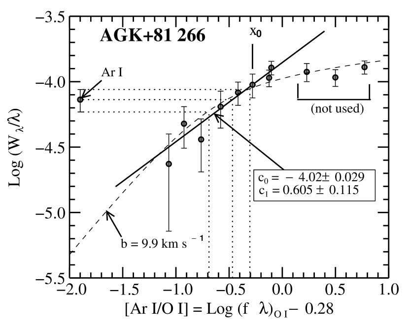
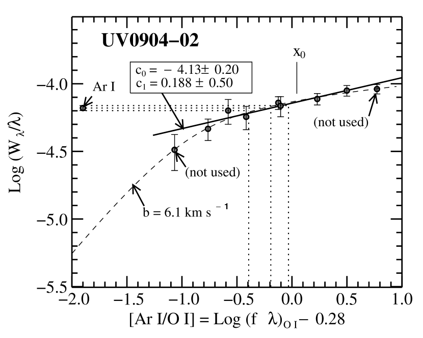
Figure 2: Examples of how the values of [Ar I/O I] are derived for the two stars chosen for Fig. 1. The equality shown in each $x$-axis label applies to the horizontal projection of the Ar I line strength onto the O I curve of growth, as expressed in Eq. 1. We performed weighted least-squares linear fits for the logarithms of $W_{\lambda}/\lambda$ for lines of O I that are most influential in establishing the trends (solid lines) for a comparison with the measurements of $\log W_{\lambda}/\lambda$ of the Ar I line. Values for $c_{0}$ and $c_{1}$ given in Eq. 2 that define these trends are shown in the boxes. The best-fit curves of growth together with their $b$ values are also shown, but they are not used in the derivations. O I lines that had strengths that were well above or below those in the important portion of curve of growth were not included in the derivation of the best fits, and they are indicated here as “(not used).” These unused lines are identified with parentheses around the equivalent width values listed in Table 1.

To determine the strength of the hypothetical O I line, we perform a weighted least-squares linear fit for $\log(W_{\lambda}/\lambda)$ vs. the quantity on the right-hand side of Eq. 1 (the abscissa for each plot in Fig. 2) for an appropriate selection of O I lines. [As with the Ar I line the $f$-values of the O I transitions are from Morton (2003).] The lines that are chosen for this fit are ones that are situated not too far from the horizontal projection (shown by dotted lines in the figure) of $\log(W_{\lambda}/\lambda)$ for the single line of Ar I onto the trend for the O I lines. With this restricted fit, we define a simple relationship in $\log(W_{\lambda}/\lambda)$ that is a good approximation to a relevant portion of the curve of growth.

In the two panels of Fig. 2, these best-fit linear trends are shown by the straight solid lines. They depict the relation between $y=\log W_{\lambda}/\lambda$ and $x=\log(f\lambda)-0.28$ according to the equation

$$y=c_{0}+c_{1}(x-x_{0}),$$ (2)

where

$$x_{0}=\sum_{i}x_{i}\sigma(y)_{i}^{-2}\Big{/}\sum_{i}\sigma(y)_{i}^{-2}$$ (3)

represents a zero reference point that produces a vanishing covariance for the errors in the fitting coefficients $c_{0}$ and $c_{1}$. A nominal value on the $x$ axis for the projection of $y_{\rm Ar~{}I}$ onto the linear relation is given by

$$x_{\rm Ar~{}I}=x_{0}+{y_{\rm Ar~{}I}-c_{0}\over c_{1}}$$ (4)

In the fraction part of this equation, the numerator and denominator have errors $(\sigma(y_{\rm Ar~{}I})^{2}+\sigma(c_{0})^{2})^{0.5}$ and $\sigma(c_{1})$, respectively. A conventional approach for deriving the error of the quotient is to add in quadrature the relative errors of the two terms, yielding the relative error of the quotient. However, this scheme breaks down when the error in the denominator is not very much less than the denominator itself. A more robust way to derive the error of a quotient has been developed by Geary (1930); for a concise description of this method see Appendix A of Jenkins (2009). We use this method here; it is effective as long as there is little chance that the denominator minus its error could become very close to zero or be negative, i.e., ${\rm denom.}/\sigma({\rm denom.})\gtrsim 3$.

The dotted lines in Figure 2 show schematically how the best fit values and the error ranges for [Ar I/O I] are derived. Note that the horizontal and vertical segments for the error limits do not exactly intersect the best linear trend for the O I lines because the error analysis allows for the uncertainty for the location of this line. (But we point out that the intersections for the worst possible error in one direction for $y_{\rm Ar~{}I}$ do not occur at the locations for the worst possible deviations in the opposite direction for the trend line.) Also, the final errors for $[{\rm Ar~{}I}/{\rm O~{}I}]=x_{\rm Ar~{}I}$ are not symmetrical about the best values. On average, the upward error bounds are about 75% as large as the negative ones.

The difference in atomic weights of Ar and O will cause the thermal contributions to the Doppler broadenings of these two elements to differ from each other. The impact of this effect on our results for the column density ratios is small however. For instance, if we consider that we are viewing absorption lines arising from the warm, neutral medium (WNM) and there were no bulk motions of the gas, the line broadening parameters $b_{\rm therm.}$ caused by thermal Doppler broadening for $T=7000\,$K would be 2.7 and $1.7\,{\rm km~{}s}^{-1}$ for O I and Ar I, respectively. For a typical observation, such as the one for AGK+81 266 illustrated in the left-hand panel of Fig. 2, we find that the observed curve of growth for the O I lines, yielding an apparent $b_{\rm obs.}=9.9\,{\rm km~{}s}^{-1}$, indicates that kinematic effects arising from turbulent motions (or multiple velocity components) should be the most important contribution to the broadening since $b_{\rm turb.}=\sqrt{b_{\rm obs.}^{2}-b({\rm O~{}I})_{\rm therm.}^{2}}=9.53\,{\rm km~{}s}^{-1}$ is only slightly smaller than $b_{\rm obs.}$. The curve of growth that characterizes the saturation of the Ar I line would conform to a slightly lower velocity dispersion parameter compared to that observed for O I, $b_{\rm obs.}=\sqrt{b_{\rm turb.}^{2}+b({\rm Ar~{}I})_{\rm therm.}^{2}}=9.68\,{\rm km~{}s}^{-1}$, because the higher atomic weight of Ar causes the thermal contribution to be smaller. For the observed equivalent width of the Ar I line, the error in the ratio of column densities caused by our assumption that the values of $b_{\rm obs.}$ of the two elements are identical will create an underestimate of $[{\rm Ar~{}I/O~{}I}]=-0.012\,$dex. A similar calculation for the more extreme line saturation exhibited by UV0904$-$02 shown in the right-hand panel of Fig. 2 indicates that the perceived outcome for [Ar I/O I] could be too low by $-0.12\,$dex. Cases showing this much saturation are rare for our collection of sight lines.

If the kinematic line broadening is not an approximately Gaussian form that one would expect from pure turbulent broadening, but instead results from distinct and well-separated narrow components, the errors in [Ar I/O I] could be larger than those evaluated above. However, the recordings of Ar I lines for 9 different stars made by IMAPS at a resolution of $4\,{\rm km~{}s}^{-1}$ that were shown by SJ98 reveal profiles that, while not exactly Gaussian, are nevertheless generally smooth and devoid of any narrow spikes that are isolated from each other. Thus, the numerical estimates presented in the above paragraph should be reasonably accurate.

One might question whether or not errors in the adopted $f$-values could cause global systematic errors in the evaluations of [Ar I/O I]. While Morton (2003) listed a very small uncertainty for the $f$-value of the Ar I line at 1048.220 Å, he did not specify errors for the O I lines. Nevertheless, empirical evidence from high quality FUSE observations of WD stars by Hébrard et al. (2002), Sonneborn et al. (2002) and Oliveira et al. (2003) all showed curves of growth that are remarkably well behaved for the same lines that are used in the present study. While one could still pose the objection that all of the O I lines could collectively have a systematic error of a certain magnitude, and yet could still yield acceptable curves of growth, this seems unlikely: the values of [O I/H I] derived by Sonneborn et al. (2002) and Oliveira et al. (2003) are generally consistent with those found elsewhere in the ISM based on measurements of the intersystem O I line at 1355.6 Å (Jenkins 2009). [Hébrard et al. (2002) did not attempt to measure $N$(H I).]

4.2.3 Outcomes

Table 2 shows the outcomes of our analysis for all of the targets in the survey, along with the applicable Galactic coordinates and apparent magnitudes of the stars. The last two columns present some cautions in numerical form. First, Column (9) lists for the fraction part of Eq. 4 the denominator divided by its error. If this number is less than about 3, the upper limit for [Ar I/O I] should not be trusted. Second, Column (10) lists the probability of obtaining a worse fit of the O I lines to the linear trend (i.e., a higher value for $\chi^{2}$), given the errors that we derived. A plot of the frequency of all of these numbers shows a distribution that is consistent with a uniform distribution between 0 and 1, which indicates that our error estimates for $W_{\lambda}$ of the O I lines are neither too conservative nor too generous. Thus, any individual case where this probability is low should not be considered as a real anomaly.

Figure 3: Outcomes for [Ar /O I] sorted according to their best values.

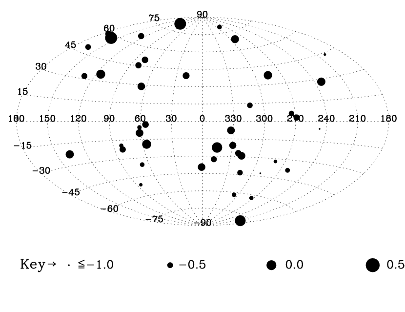
Figure 4: Locations of the stars and their values of [Ar I/O I] shown on an Aitoff projection of Galactic coordinates. The sizes of the black circles indicate the values of [Ar I/O I] according to the key shown at the bottom.

Figure 3 shows a graphic representation of all of the results and their uncertainties. They were ranked and then arranged in order of the best values of [Ar I/O I] to make it easier to see the dispersion of results and also to show that the more extreme deviations often represent cases where the errors are somewhat larger than normal.

Table 2: Results for [Ar I/O I]

	Galactic Coord.				[Ar I/O I]
Star	$\ell$	$b$			Lower	Best	Upper	Denom. Val.	Prob. of
Name	(deg.)	(deg.)	$m_{B}$	$m_{V}$	Limit	Value	Limit	/Error	Worse Fit
(1)	(2)	(3)	(4)	(5)	(6)	(7)	(8)	(9)	(10)
2MASSJ15265306+7941307	$115.06$	$34.93$	$11.30$	$11.60$	$-0.45$	$-0.11$	$0.14$	$4.74$	$0.26$
AA Dor	$280.48$	$-32.18$	$10.84$	$11.14$	$-1.18$	$-0.76$	$-0.51$	$2.60$	$0.70$
AGK+81 266	$130.67$	$31.95$	$11.60$	$11.94$	$-0.69$	$-0.47$	$-0.30$	$5.25$	$0.89$
BD+18 2647	$289.48$	$80.14$	$11.48$	$11.82$	$-1.14$	$-0.63$	$-0.34$	$3.76$	$0.66$
BD+25 4655	$81.67$	$-22.36$	$9.39$	$9.68$	$-1.25$	$-0.44$	$-0.02$	$4.68$	$0.80$
BD+28 4211	$81.87$	$-19.29$	$10.17$	$10.51$	$-1.03$	$-0.69$	$-0.44$	$7.42$	$0.07$
BD+37 442	$137.07$	$-22.45$	$9.69$	$9.92$	$-0.32$	$-0.20$	$-0.02$	$2.54$	$0.04$
BD+39 3226	$65.00$	$28.77$	$9.89$	$10.18$	$-0.49$	$-0.28$	$-0.10$	$3.42$	$0.69$
CPD$-$31 1701	$246.46$	$-5.51$	$10.22$	$10.56$	$-1.69$	$-1.04$	$-0.70$	$4.68$	$0.42$
CPD$-$71 172	$290.20$	$-42.61$	$10.90$	$10.68$	$-2.60$	$-1.46$	$-0.94$	$2.28$	$0.77$
EC11481-2303	$285.29$	$37.44$	$11.49$	$11.76$	$-0.53$	$-0.18$	$0.11$	$4.81$	$0.43$
Feige 34	$173.32$	$58.96$	$10.84$	$11.18$	$-1.16$	$-0.42$	$0.02$	$3.43$	$0.82$
HD113001	$110.97$	$81.16$	$9.65$	$9.65$	$-0.26$	$0.23$	$0.63$	$4.12$	$0.42$
JL 119	$314.61$	$-43.36$	$13.22$	$13.49$	$-0.63$	$-0.53$	$-0.45$	$5.68$	$0.16$
JL 25	$318.63$	$-29.17$	$13.09$	$13.28$	$-0.94$	$-0.27$	$0.20$	$3.54$	$0.29$
JL 9	$322.60$	$-27.04$	$12.96$	$13.24$	$-0.68$	$-0.43$	$-0.22$	$5.12$	$0.24$
LB 1566	$306.36$	$-62.02$	$12.81$	$13.13$	$-0.89$	$-0.65$	$-0.48$	$3.06$	$0.82$
LB 1766	$261.65$	$-37.93$	$\cdots$	$12.34$	$-1.03$	$-0.62$	$-0.34$	$4.71$	$0.07$
LB 3241	$273.70$	$-62.48$	$12.45$	$12.73$	$-0.86$	$-0.69$	$-0.55$	$7.98$	$0.01$
LS 1275	$268.96$	$2.95$	$10.94$	$11.40$	$-1.01$	$-0.44$	$0.00$	$4.69$	$0.77$
LSE 234	$329.44$	$-20.52$	$\cdots$	$12.63$	$-0.77$	$-0.34$	$0.00$	$3.70$	$0.38$
LSE 259	$332.36$	$-7.71$	$\cdots$	$12.54$	$-0.40$	$-0.26$	$-0.12$	$2.52$	$0.08$
LSE 263	$345.24$	$-22.51$	$11.40$	$11.30$	$-0.27$	$0.07$	$0.37$	$6.32$	$0.24$
LSE 44	$313.37$	$13.49$	$12.21$	$12.45$	$-0.73$	$-0.52$	$-0.34$	$5.53$	$0.11$
LSII +18 9	$55.20$	$-2.65$	$11.81$	$12.13$	$-0.65$	$-0.40$	$-0.21$	$2.43$	$0.66$
LSII +22 21	$61.17$	$-4.95$	$12.23$	$12.58$	$-1.06$	$-0.67$	$-0.41$	$4.04$	$0.91$
LSIV +10 9	$56.17$	$-19.01$	$11.71$	$11.98$	$-0.18$	$-0.10$	$-0.03$	$11.01$	$0.21$
LSS 1362	$273.67$	$6.19$	$12.27$	$12.50$	$-0.60$	$-0.53$	$-0.48$	$7.05$	$0.65$
MCT 2005$-$5112	$347.71$	$-32.68$	$15.20$	$\cdots$	$-0.63$	$-0.47$	$-0.36$	$3.82$	$0.46$
MCT 2048$-$4504	$1.10$	$-39.51$	$14.85$	$15.20$	$-0.52$	$-0.28$	$-0.09$	$4.97$	$0.97$
NGC6905 star	$61.49$	$-9.57$	$16.30$	$14.50$	$-0.46$	$-0.26$	$-0.12$	$2.56$	$0.75$
PG0919+272	$200.46$	$43.89$	$12.27$	$12.69$	$-2.24$	$-0.89$	$-0.16$	$3.83$	$0.64$
PG0952+519	$164.07$	$49.00$	$12.47$	$12.80$	$-0.60$	$-0.51$	$-0.44$	$5.11$	$0.90$
PG1032+406	$178.88$	$59.01$	$10.80$	$\cdots$	$-3.79$	$-1.84$	$-0.41$	$2.71$	$0.30$
PG1051+501	$159.61$	$58.12$	$14.59$	$\cdots$	$-0.01$	$0.28$	$0.59$	$2.77$	$0.61$
PG1230+068	$290.42$	$68.85$	$12.25$	$\cdots$	$-0.57$	$-0.23$	$0.06$	$7.58$	$0.03$
PG1544+488	$77.54$	$50.13$	$12.80$	$\cdots$	$-0.48$	$-0.40$	$-0.34$	$5.41$	$0.56$
PG1605+072	$18.99$	$39.33$	$13.01$	$12.84$	$-0.52$	$-0.36$	$-0.24$	$5.31$	$0.88$
PG1610+519	$80.50$	$45.31$	$13.73$	$\cdots$	$-0.53$	$-0.44$	$-0.36$	$10.93$	$0.22$
PG2158+082	$67.58$	$-35.48$	$12.66$	$\cdots$	$-0.91$	$-0.64$	$-0.49$	$2.78$	$0.16$
PG2317+046	$84.84$	$-51.10$	$\cdots$	$12.87$	$-1.42$	$-0.79$	$-0.37$	$4.20$	$0.04$
Ton 102	$127.05$	$65.78$	$13.29$	$13.54$	$-0.89$	$-0.45$	$-0.15$	$2.96$	$0.31$
Ton S227	$201.39$	$-77.81$	$11.60$	$11.90$	$-0.34$	$0.12$	$0.44$	$9.06$	$0.36$
UV0904$-$02	$232.98$	$28.12$	$11.64$	$11.96$	$-0.39$	$-0.19$	$-0.03$	$3.78$	$0.93$

Figure 4 shows the locations of the targets in the sky and their respective values of [Ar I/O I]. While no obvious regional trends seem to be evident, we can perform a test to determine whether or not the variability of the outcomes exceeds what we would have expected from our errors (assuming that they are correct). We do this by computing a value for $\chi^{2}$, where the choice for the error of each case depends on whether a test value is above or below the measurement outcome. This procedure properly takes into account the asymmetries of the errors. Adopting this method, we find that a minimum $\chi^{2}$ of 66.9 for the 44 measurements occurs at a value $[{\rm Ar~{}I/O~{}I}]=-0.438$. This minimum for the $\chi^{2}$ with 43 degrees of freedom is greater than what we would have expected from our errors alone (the probability of obtaining by chance a higher value for $\chi^{2}$ is only 1%). If we were to propose that the real variability across the sky is $\sigma=0.11~{}{\rm dex}$, and we add this value in quadrature to all of the experimental errors, the minimum $\chi^{2}$ drops to 42.4, which makes the probability of a worse fit equal to 50%. The location of this new minimum is at $[{\rm Ar~{}I/O~{}I}]=-0.427$.

The discussion above has considered only the random fluctuations arising from either the measurements or the true variability in [Ar I/O I] in different sight lines. We must not lose sight of the fact that there can be an overall systematic error of 0.11 dex for the entire collection. This global error arises from the uncertainties of the value for $\log({\rm Ar/O})_{\odot}$ that went into Eq. 1. It is much larger than the error in the weighted mean value for all of the measurements.

5 ARE THE STARS BEYOND THE BOUNDARY OF THE LOCAL BUBBLE?

As discussed in Section 2, our objective is to sample interstellar material that is beyond the edge of the Local Bubble, enough so that our measurements are not heavily influenced by the very low density gas within this cavity. In principle, we could compare the three-dimensional locations of the target stars with maps that outline the boundary of the Local Bubble (Vergely et al. 2010; Welsh et al. 2010; Reis et al. 2011) to indicate whether or not we are primarily sampling gas in the surrounding denser medium. However, the distances to our targets are uncertain, which makes this approach unworkable. Instead, we adopt a definition of the boundary proposed by Sfeir et al. (1999) (and one that was also used by Lehner et al. (2003)), who linked its location to the sudden onset of Na I D-line absorption that crossed a threshold $W_{\lambda}({\rm D2})=20\,$mÅ. This threshold is equivalent to $N({\rm H~{}I})\approx 2\times 10^{19}{\rm cm}^{-2}$ (Ferlet et al. 1985), which in turn corresponds to $N({\rm O~{}I})$ that is slightly greater than $10^{16}{\rm cm}^{-2}$. Lehner et al. (2003) found that a typical velocity dispersion parameter $b({\rm O~{}I})=6\,{\rm km~{}s}^{-1}$ occurred inside the Local Bubble. Using these two parameters for O I, $(N,~{}b)=(10^{16}{\rm cm}^{-2},~{}6\,{\rm km~{}s}^{-1})$, we can compute the equivalent widths for all of the O I lines when the boundary is crossed. The third row of numbers in the column headings in Table 1 shows the values of $W_{\lambda}$ (in mÅ) for all but the strongest three lines. By comparing these values with the entries that show our measurements, particularly the weaker but securely measured ones, we can ascertain that our targets are beyond the edge of the Local Bubble.

6 INTERPRETATION: FUNDAMENTAL PROCESSES AND EQUATIONS

In this section, we address the basic physical processes that relate our findings on [Ar I/O I] to the ionization balance of the gas and the resulting degree of partial ionization. Our discussion about the means of ionizing the atoms will focus mainly on the primary ionization by photons, along with the effects of collisional ionizations caused by secondary electrons that originate from these primary ionizations. These two processes are the most important sources of ionization, and they represent one side of the balance between recombinations with free electrons and charge exchange reactions between various constituents of the medium. For completeness, we will also cover other means of ionizing atoms and creating free electrons, such as cosmic ray ionizations, the ionizations of inner shell electrons of heavy elements by X-rays, the creation of ionizing photons when helium ions recombine, and the nearly complete ionization of many elements that have first ionization potentials below that of hydrogen.

6.1 Direct and Secondary Ionizations of H and Ar

6.1.1 Photoionization

The primary photoionization cross sections for neutral Ar are larger than those for H by about one order of magnitude at low energies, and the ratio increases substantially at higher energies. Various secondary ionizing processes initiated by the primary photoionizations of H and He likewise have a stronger effect on Ar than on H. This contrast in ionization rates is the fundamental tool that we use in the interpretation of the Ar data to quantify the photoionization of H and the subsequent creation of free electrons. For the collective effect of all of these ionization channels, we can construct a simple formalism based on arguments created by SJ98. They defined a quantity based on ionization rates $\Gamma$ and recombination coefficients $\alpha$ for the two elements,

$$P_{\rm Ar}={\Gamma({\rm Ar}^{0})\alpha({\rm H}^{0},T)\over\Gamma({\rm H}^{0})\alpha({\rm Ar}^{0},T)}~{}.$$ (5)

SJ98 considered only primary photoionizations of these two elements. Going beyond their development, we construct a more comprehensive picture by considering some refinements in the calculations of $\Gamma$ for both ${\rm H}^{0}$ and ${\rm Ar}^{0}$.

First, we start with the primary photoionization rates $\Gamma_{p}=\int F(E)\sigma(E)dE$, where $F(E)$ is the ambient photon flux as a function of energy $E$ and $\sigma(E)$ is the photoionization cross section for either H⁰ (Spitzer 1978, pp. 105-106) or Ar⁰ (Marr & West 1976). Next, we include secondary ionizations with rates $\Gamma_{s}$ that are created by the collisions from energetic electrons that are liberated by the primary photoionizations of H and He. Added to this are the effects from photons with energies above about 300 eV, which can interact with the abundant heavy elements in the ISM to produce additional energetic electrons that will ionize H and Ar with a rate that we identify as $\Gamma_{s^{\prime}}$. These electrons arise from the primary ionizations of the inner electronic shells, and they are supplemented by one or more additional electrons from the Auger process. Finally, we must acknowledge that recombinations of singly- and doubly-ionized He ions with electrons create additional photons when de-excitation occurs in the lower stage of ionization, either He⁰ or He⁺. The importance of not overlooking secondary electrons and recombination photons from the He ionizations is underscored by the fact that while the abundance of He is only 1/10 that of hydrogen, its primary ionization cross section is 6 to 100 times that of H over the energy range 25 to 4000 eV. Most of the recombination photons are capable of ionizing both H and Ar, and they supplement the other sources of ionization with rates $\Gamma_{He^{0}}$ and $\Gamma_{He^{+}}$. In short, we consider that the total ionization rates for the two elements in Eq. 5 each consist of five contributions,

$$\Gamma=\Gamma_{p}+\Gamma_{s}+\Gamma_{s^{\prime}}+\Gamma_{He^{+}}+\Gamma_{He^{0}}$$ (6)

The details of how we compute $\Gamma_{s}$, $\Gamma_{s^{\prime}}$, $\Gamma_{He^{+}}$ and $\Gamma_{He^{0}}$ are discussed in Appendices A and B.

The quantity $P_{\rm Ar}$ defined in Eq. 5 provides a means for evaluating how large the neutral fraction of Ar should be relative to that of H according to the formula

$$[{\rm Ar~{}I/H~{}I}]=\log\left[{1+n({\rm H}^{+})/n({\rm H}^{0})\over 1+P_{\rm Ar}n({\rm H}^{+})/n({\rm H}^{0})}\right].$$ (7)

For a more accurate formulation of [Ar I/H I] that will be developed later in Section 6.4, we will introduce a more refined parameter $P^{\prime}_{\rm Ar}$ that will be based on a calculation that is more elaborate than the one shown in Eq. 5. This new parameter will be substituted for $P_{\rm Ar}$ in Eq. 7. Under most conditions, the differences between $P^{\prime}_{\rm Ar}$ and $P_{\rm Ar}$ are small.

Figure 5 shows for both H and Ar the monoenergetic cross sections for primary ionization (dashed lines), the effective enhancements arising from the secondary ionizations $\Gamma_{s}$ (dash-dot lines) for $x_{e}=0.05$, and the additional effects from $\Gamma_{s^{\prime}}$, $\Gamma_{He^{+}}$ and $\Gamma_{He^{0}}$, all of which give total ionization rates shown by the solid lines. For H, secondary ionizations outweigh the primary ones for photon energies above about 100 eV. By contrast, we find that for Ar the enhancement at these energies is small compared to its much higher primary cross section. A more narrowly defined version of $P_{\rm Ar}$, which we denote as $P_{\rm Ar}(E)$, applies to an irradiation of the gas by photons of a given energy $E$, rather than from a combination of fluxes over a broad energy range. The definition of $P_{\rm Ar}(E)$ is illustrated in the upper panel of the figure, and its dependence on $E$ is shown in the bottom panel.

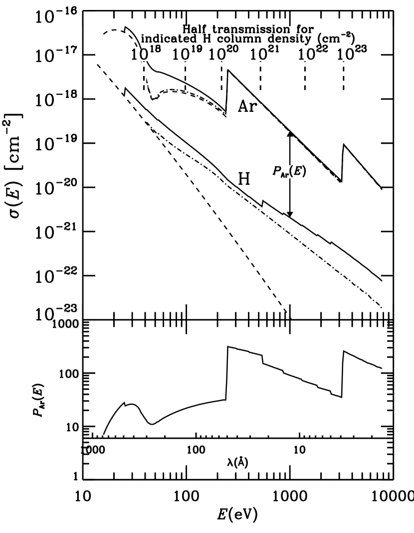
Figure 5: Upper panel: Various combinations of effective photoionization cross sections for neutral hydrogen and argon as a function of energy $E$. The dashed lines depict the absorption cross sections for the primary ionization rates $\Gamma_{p}$ that would apply to monoenergetic radiation at the energy $E$ shown on the $x$-axis. The effective cross sections that arise by including the additional effects from ionizations by secondary electrons produced by H and He (related to $\Gamma_{s}$) are shown by the dot-dash lines. These secondary ionization efficiencies were calculated according to the principles outlined in Section A.1 of the Appendix for an electron fraction $x_{e}=0.05$.; see Eqs. A1 and A2. These two ionization processes can be further enhanced by photons that come from recombinations of He ions with free electrons (Appendix B) and electrons from inner shell ionizations of heavy elements (Appendix A.2), leading to total effective cross sections depicted by the solid lines. Across the top of the plot are markers showing the energies at which half-intensity penetration depths for the photons occur for various hydrogen column densities, assuming the gases have a solar abundance ratio for various elements. The quantity $P_{\rm Ar}(E)$ defined in Eq. 5 for a specific energy $E$ is approximately equal to the ratio of the total effective photoionization cross sections that give rise to $\Gamma({\rm H}^{0},~{}{\rm Ar}^{0})$ defined in Eq. 6, since the recombination rates for the two elements are about the same for all temperatures. Bottom panel: A plot of $P_{\rm Ar}(E)$ as a function of energy.

6.1.2 Other Ionization Mechanisms

As discussed earlier in Section 1, neutral atoms in the ISM are subjected to ionization by cosmic ray particles. These ionizations, with a rate $\zeta_{\rm CR}$, add to the effects of primary and secondary ionizations from photons discussed above. To obtain proper values of $\zeta_{\rm CR}$ that apply to the diffuse medium, we must apply corrections to the values of $\zeta_{\rm CR}$ that were measured for the more dense media that have appreciable concentrations of molecules. The details of this computation are discussed in Appendix C.

In the WNM, the main source of free electrons is from the ionization of H and He. However, a small number of additional electrons arise from other atoms that can be ionized by starlight photons less energetic than the ionization potential of H. For the combined effect from these elements, we adopt an estimate $n({\rm M}^{+})$ equal to $1.5\times 10^{-4}$ times the density of hydrogen based on the assumption that the gas we are viewing is in a regime where the element depletions are relatively modest.

6.2 Recombination

The radiative recombination coefficients for free electrons and ions to create neutral hydrogen and singly-ionized helium, $\alpha({\rm H}^{0},T)$ and $\alpha({\rm He}^{+},T)$, are taken from Spitzer (1978, pp. 105-107). For $\alpha({\rm H}^{0})$, we excluded recombinations to the lowest electronic level, since they generate Lyman limit photons that can re-ionize hydrogen atoms over a short distance scale. Recombination coefficients for He⁰ were taken from Aldrovandi & Péquignot (1973) and those for Ar⁰ from Shull & Van Steenberg (1982). The results for Ar⁰ given by Shull & Van Steenberg (1982) agree well with the radiative recombination coefficients listed by Aldrovandi & Péquignot (1974). The minimum temperature where dielectronic recombination for Ar⁰ becomes important is $2.5\times 10^{4}\,$K (Aldrovandi & Péquignot 1974), which is above temperatures that we will consider, hence we can ignore this process.

In addition to recombining with a free electron, an ion can also be neutralized by colliding with a dust grain and removing an electron from it (Snow 1975; Draine & Sutin 1987; Lepp et al. 1988; Weingartner & Draine 2001a). The operation of this effect on protons is important for regulating the fraction of free electrons in the cold neutral medium (CNM), but it is of lesser significance for the WNM [cf. Figs. 16.1 and 16.2 of Draine (2011)], which probably dominates the sight lines in our study. The rate constant $\alpha_{g}$ for this process is normalized to the local hydrogen density $n({\rm H_{tot}})\equiv n({\rm H}^{0})+n({\rm H}^{+})$, and it depends on several physical parameters that influence the charge on the grains, such as the electron density $n(e)$, the rate of photoelectric emission that is driven by the intensity $G$ of the local radiation field between 6 and 13.6 eV, and the temperature $T$. For our equilibrium equations in Section 6.4, we have adopted parametric fits for $\alpha_{g}({\rm H}^{0},n(e),G,T)$ and $\alpha_{g}({\rm He}^{0},n(e),G,T)$ from Weingartner & Draine (2001a). They do not supply fit coefficients for $\alpha_{g}({\rm Ar}^{0},n(e),G,T)$, but since the ionization potential of Ar⁰ is close to that of H⁰, it is reasonable to adopt the hydrogen rate coefficient and divide it by the square-root of the atomic weight (40) of Ar. Throughout our analysis, we set $G=1.13$, which is the value recommended for the general ISM by Weingartner & Draine (2001a).

6.3 Charge Exchange

In addition to the recombination processes mentioned in the previous section, charge exchange reactions with neutral hydrogen can also lower the ionization state of an atom. With reference to such reactions for element X, ${\rm X}^{+}+{\rm H}^{0}\rightarrow{\rm X}^{0}+{\rm H}^{+}$ and ${\rm X}^{++}+{\rm H}^{0}\rightarrow{\rm X}^{+}+{\rm H}^{+}$, we adopt the notation $C^{\prime}({\rm X}^{+},T)$ and $C^{\prime}({\rm X}^{++},T)$ for the respective rate constants. For our calculations of $C^{\prime}({\rm He}^{+},T)$, $C^{\prime}({\rm He}^{++},T)$, $C^{\prime}({\rm Ar}^{+},T)$, and $C^{\prime}({\rm Ar}^{++},T)$, we adopted Kingdon & Ferland’s (1996) fits to the calculations from various sources (see their Table 1 for the coefficients and references).

Since the ionization potential of neutral oxygen is close to that of hydrogen, the rate constant for charge exchange of these two species is large and reverse endothermic reaction is not negligible, except at very low temperatures. The rate constant $C({\rm O}^{+},T)$ for the reaction ${\rm O}^{0}+{\rm H}^{+}\rightarrow{\rm O}^{+}+{\rm H}^{0}$ can be obtained from $C^{\prime}({\rm O}^{+},T)$ by the principle of detailed balancing. However, in doing so, one must treat the three fine-structure levels of the ground state of O⁰ separately, since their energy separations are comparable to the differences in the ionization potentials of H and O. The large rate constants in both directions (Stancil et al. 1999) assures that the ionization fraction of O is locked very close to a value 8/9 times that of H for $T\gtrsim 10^{3}\,$K. This is a key principle that allows us to use O as a substitute for H in the present study or Ar vs. H fractional ionizations.

For completeness, we should also consider charge exchange reactions between Ar and He, even though the abundance of He is much lower than that of H. The charge transfer recombination reaction ${\rm Ar}^{++}+{\rm He}^{0}\rightarrow{\rm Ar}^{+}+{\rm He}^{+}$ has a rate constant $D^{\prime}({\rm Ar}^{++},T)=1.3\times 10^{-10}{\rm cm}^{3}{\rm s}^{-1}$ according to Butler & Dalgarno (1980), which they claim to be constant for $T\geq 10^{3}\,$K. The charge transfer ionization reaction with He⁺, i.e., ${\rm Ar}^{0}+{\rm He}^{+}\rightarrow{\rm Ar}^{+}+{\rm He}^{0}$, has a rate constant $D({\rm Ar}^{+},T)<10^{-13}{\rm cm}^{3}{\rm s}^{-1}$ according to Albritton (1978), so we will ignore this process in the equation for the ionization balance for Ar (Eq. 8 below).

6.4 Equilibrium Equations

In a medium where both hydrogen and helium are partly ionized, the densities of an element X in its 3 lowest levels of ionization X⁰, X⁺ and X⁺⁺ are governed by the equilibrium equations

$$\Big{[}\Gamma({\rm X}^{0})+\zeta_{\rm CR}({\rm X}^{0})+C({\rm X}^{+},T)n({\rm H^{+}})\Big{]}n({\rm X}^{0})$$ (8)

$$= \Big{[}\alpha({\rm X}^{0},T)n(e)+C^{\prime}({\rm X}^{+},T)n({\rm H}^{0})$$

$$+ \alpha_{g}({\rm X}^{0},n(e),G,T)n({\rm H_{tot}})\Big{]}n({\rm X}^{+})$$

and

$$\Gamma({\rm X}^{+})n({\rm X}^{+})=\Big{[}\alpha({\rm X}^{+},T)n(e)+C^{\prime}({\rm X}^{++},T)n({\rm H}^{0})$$ (9)

$$+ D^{\prime}({\rm X}^{++},T)n({\rm He}^{0})\Big{]}n({\rm X}^{++})$$

where $\Gamma({\rm X}^{y})$ is the photoionization rate of element X in its ionization state $y$ (neutral, +, or ++) and $\alpha({\rm X}^{y},T)$ is the recombination rate of the $y+1$ state with free electrons as a function of temperature $T$. The simultaneous solution to these two equations yields the fractional abundances in the three ionization levels

$$f_{0}({\rm X},T)\equiv{n({\rm X}^{0})\over n({\rm X}^{0})+n({\rm X}^{+})+n({\rm X}^{++})}=\Bigg{(}1\,+$$

$${\Big{[}\Gamma({\rm X}^{0})+\zeta_{\rm CR}({\rm X}^{0})+C({\rm X}^{+},T)n({\rm H^{+}})\Big{]}\Big{[}\Gamma({\rm X}^{+})+Y\Big{]}\over\Big{[}\alpha({\rm X}^{0},T)n(e)+C^{\prime}({\rm X}^{+},T)n({\rm H}^{0})+\alpha_{g}({\rm X}^{0},n(e),G,T)n({\rm H_{tot}})\Big{]}Y}\Bigg{)}^{-1}$$ (10a)

with

$$Y=\alpha({\rm X}^{+},T)n(e)+C^{\prime}({\rm X}^{++},T)n({\rm H}^{0})+D^{\prime}({\rm X}^{++},T)n({\rm He}^{0})~{},$$ (10b)

$$f_{++}({\rm X},T)\equiv{n({\rm X}^{++})\over n({\rm X}^{0})+n({\rm X}^{+})+n({\rm X}^{++})}={1-f_{0}({\rm X},T)\over 1+Y/\Gamma({\rm X}^{+})}~{},$$ (11)

and

$$f_{+}({\rm X},T)\equiv{n({\rm X}^{+})\over n({\rm X}^{0})+n({\rm X}^{+})+n({\rm X}^{++})}=1-f_{0}({\rm X},T)-f_{++}({\rm X},T)~{}.$$ (12)

6.5 Electron Density and the Ionization Fractions of H and He

Before the ionization fractions of Ar can be derived, we must determine not only the ionization balance of hydrogen, but also that for helium. We do this by solving Eqs. 6.4–12 (substituting He for X and eliminating the $D^{\prime}$ term) along with the equation for the hydrogen ionization balance,

$${n({\rm H}^{+})\over n({\rm H}^{0})}={\Gamma({\rm H}^{0})+\zeta_{\rm CR}({\rm H}^{0})+Z\over\alpha({\rm H}^{0},T)n(e)+\alpha_{g}({\rm X}^{0},n(e),G,T)n({\rm H_{tot}})-Z}~{},$$ (13a)

with

$$Z=0.1n({\rm H}^{0})\big{[}C^{\prime}({\rm He}^{+},T)f_{+}({\rm He},T)+C^{\prime}({\rm He}^{++},T)f_{++}({\rm He},T)\big{]}~{},$$ (13b)

and the constraints

$$n({\rm He}^{0})+n({\rm He}^{+})+n({\rm He}^{++})=0.1n({\rm H}^{0})\left[1+{n({\rm H}^{+})\over n({\rm H}^{0})}\right]$$ (14)

and

$$n(e)=n({\rm H}^{+})+n({\rm He}^{+})+2n({\rm He}^{++})+n({\rm M}^{+})~{}.$$ (15)

Since the hydrogen ionization balance depends on $n(e)$ which in turn is influenced by the ionization fractions of He (which are also influenced by $n(e)$), we must solve Eqs. 13a-15 iteratively to obtain a solution. We found that these equations converged very well if we kept $n({\rm H_{tot}})$ and the ionization rate of H pegged to a certain value. Starting with a zero helium ionization rate, the iterations progressed slowly to successively higher rates until the final, correct value was reached and the ionization fractions had stabilized.

After obtaining the final results for the coupled hydrogen and helium ionization balances, we can solve for $f_{0}({\rm Ar})$ using Eq. 6.4. This result can then be used to derive a more accurate value for $P_{\rm Ar}$,

$$P^{\prime}_{\rm Ar}={n({\rm H}^{0})\over n({\rm H}^{+})}\left({1\over f_{0}({\rm Ar})}-1\right)~{},$$ (16)

which can be substituted for $P_{\rm Ar}$ in Eq. 7 to obtain a solution for [Ar I/H I] that makes use of all of the physical processes that were discussed in Sections 6.1–6.3.

7 OUTCOME FROM KNOWN SOURCES OF PHOTOIONIZATION

7.1 External Radiation

Over many decades, the diffuse, soft X-ray background has been measured by a large number of different experiments [for a review, see McCammon & Sanders (1990)]. Most of the emission below 1 keV arises from hot ($T>10^{6}\,$K) gas in the Galactic disk and halo, with radiation from extragalactic sources dominating at higher energies (Chen et al. 1997; Miyaji et al. 1998; Moretti et al. 2009). Much of the literature on the diffuse radiation shows a distinction between contributions from a local component with little foreground absorption and more distant emissions with varying levels of absorption. The local background was once identified as having originated from hot gas in the Local Bubble (Sanders et al. 1977; Hayakawa et al. 1978; Fried et al. 1980), but in recent years it has been recognized to be strongly contaminated, or completely dominated, by X-rays arising from charge exchange produced by the interaction of the solar wind with incoming interstellar atoms (Cravens 2000; Lallement 2004; Pepino et al. 2004; Koutroumpa et al. 2006, 2007, 2009; Peek et al. 2011; Crowder et al. 2012). For this reason, we ignore the weakly absorbed, nearly isotropic portion of the X-ray background and focus our attention to the component that exhibits a pattern in the sky that clearly shows absorption by gas in the Galaxy.

Kuntz & Snowden (2000) have performed a detailed investigation of the nonlocal component, which they call the transabsorption emission (TAE). They describe the strength and spectral character of the TAE in terms of emissions from optically thin plasmas at two different temperatures. They define a soft component that has a mean intensity over the sky $I=2.6\times 10^{-8}{\rm erg~{}cm}^{-2}{\rm s}^{-1}{\rm sr}^{-1}$ over the interval $0.1<E<2\,$keV and a spectrum consistent with the emission from a plasma at a temperature $T=10^{6.06}\,$K, and this flux is accompanied by a hard component with $I=8.5\times 10^{-9}{\rm erg~{}cm}^{-2}{\rm s}^{-1}{\rm sr}^{-1}$ over the same energy interval with $T=10^{6.46}\,$K. To translate the sum of these two components into a distribution of the photon flux as a function of energy, $F(E)$, we calculate synthetic flux representations using the CHIANTI database and software (Version 6.0) (Dere et al. 1997, 2009), after normalizing the emission measures to give the intensities stated above (we find that ${\rm EM}=10^{16.37}$ and $10^{15.81}{\rm cm}^{-5}$ for the soft and hard components, respectively). We supplement the TAE result with an underlying power-law extragalactic emission of the form $10.5\,{\rm phot~{}cm}^{-2}{\rm s}^{-1}{\rm sr}^{-1}{\rm keV}^{-1}E({\rm keV})^{-1.46}$ (Chen et al. 1997).

The ISM is opaque to X-rays at the lowest energies. The energies at which half of the X-rays are absorbed for various column densities are shown in the top portion of Figure 5, which were derived from the calculations of Wilms et al. (2000). At energies of around 100 eV where the ISM is neither completely opaque or transparent for $N({\rm H}^{0})\approx{\rm few}\,\times 10^{19}{\rm cm}^{-2}$, uncertainties in the layout of emitting and absorbing regions make it difficult to calculate with much precision how far the X-rays can penetrate the typical gas volumes that were sampled in our survey of Ar I and O I. Thus, rather than implement an elaborate attenuation function that would be difficult to explain (and perhaps not especially correct at our level of understanding), we apply a simplification that all of the X-rays are transmitted above some threshold energy and none below it. The threshold that we adopted was 90 eV, on the assumption that in some directions the gas can view the unattenuated X-ray sky through $N({\rm H}^{0})$ slightly less than $10^{19}{\rm cm}^{-2}$.

The upper panel of Figure 6 shows our synthesis of the sum of the extragalactic power-law emission and TAE synthesis described above. For the purpose of calculating $\Gamma$ for various elements, we make use of only the flux depicted by the dark trace in the figure, i.e., that which starts at the cutoff energy (90 eV) and ends at an energy beyond which no appreciable additional ionization occurs.

7.2 Internal Radiation Sources

Embedded within the ISM are sources of EUV and X-ray radiation that can make additional contributions to $\Gamma$. We can make estimates for their average space densities and the character of their emissions, but one uncertainty that remains is how well the ensuing photoionizations are dispersed throughout the ambient gas. At one extreme representing minimum dispersal, we envision the classical Strömgren Spheres that surround sources that are not moving rapidly and that emit most of their photons with barely enough energy to ionize hydrogen. These photons have a short mean free path in a neutral medium. Under these circumstances, the zone of influence of the source is sharply bounded, and the resulting ionization is nearly total inside the region and zero outside it. At the other extreme, one can imagine that the photons, ones that have relatively high energy, can travel over a significant fraction of the inter-source distances before they are absorbed. In addition, the sources themselves could move rapidly enough that they never have a chance to establish a stable condition of ionization equilibrium. (This issue will be investigated quantitatively in Section 7.5.) These conditions could lead to the ionization being more evenly distributed and not necessarily complete. If the sources have large enough velocities, we can even imagine a picture where there is a random network of “fossil Strömgren trails” (Dupree & Raymond 1983) that ultimately might blend together. More extreme manifestations of such trails in denser media may have already been discovered by McCullough & Benjamin (2001) and Yagi et al. (2012), who observed faint, but straight and narrow lines of H$\alpha$ emission in the sky (but were unable to identify the sources that created them).

It is difficult to establish where in the continuum between the two extremes for the dispersal of ionization the true effects of embedded EUV and X-ray sources are to be found. For our treatment of the influence of these production sites for ionizing radiation, we will adopt the simplified premise that all of their photons are available to create a uniform but weak level of ionization everywhere. This picture is not entirely correct, since one should expect that very near the sources some fraction of the ionizing photons are “wasted” by creating localized regions with much higher than usual levels of ionization. Such regions dissipate most of their ionization rapidly because their recombination times are short. For this reason, our making use of a calculated average production rate of ionizing photons per unit volume will lead to an equilibrium equation that overestimates the space- and time-averaged level of ionization. (Later, it will be shown that this overestimate is of no real consequence because we obtain an answer that is still below that needed to explain the overall average ionization level.)

In the sections that follow, we consider three classes of sources that are randomly distributed throughout the neutral ISM and can in principle help to ionize it: main-sequence stars, active X-ray binaries, and WD stars. Luminous, early-type stars contribute large amounts of ionizing radiation, but most of their radiation completely ionizes the surrounding media and makes the gas virtually invisible in the Ar I and O I lines. These stars also tend to be clustered inside the dense clouds of gas that led to their formation.

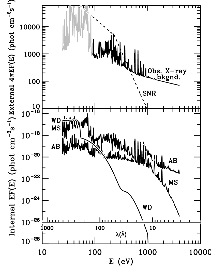
Figure 6: Upper panel: External fluxes arising from the known X-ray background radiation (solid line) and a hypothetical, time-averaged flux (over a recombination time of $\approx 1\,$Myr) from 3 supernova remnants at a distance of 100 pc (dashed line). The gray portion of the solid curve is in an energy range where the opacity to X-rays is high, and thus this radiation is not likely to penetrate into much of the gas that we observe. Lower panel: Internal average rates per unit volume for the injection of ionizing photons by the coronae of main-sequence stars (MS), active binaries (AB) and the photospheres of WD stars (WD). (A machine readable table of all 5 flux distributions vs. $E$ shown in this figure is available in the online version of the Astrophysical Journal.)

The question may arise as to whether or not, by considering the embedded sources as a separate contribution that adds to the external radiation background discussed earlier, we are possibly “double counting” some of the photons that could ionize the ISM. Kuntz & Snowden (2001) have computed the probable relative contribution of Galactic point sources that were not explicitly taken out of their measurements of the diffuse X-ray background, and they concluded that this contamination was, at most, only about $2-10\%$ of the radiation that was thought not to arise from the Local Bubble. Within their highest energy bands ($0.73-2.01\,$keV), they state that the contamination could be as high as 51%.

7.2.1 Main-sequence Stars

For various kinds of point sources, the ratio of the emission of X-rays to photons in the $V$ band is usually defined by the relation

$$\log(f_{X}/f_{V})=\log f_{X}+0.4m_{V}+5.37~{},$$ (17)

where $f_{X}$ is the apparent X-ray flux of the source over a specified energy interval, expressed in ${\rm erg~{}cm}^{-2}{\rm s}^{-1}$, and $m_{V}$ is its apparent visual magnitude. The total output of X-rays from a source with an absolute magnitude $M_{V}=0$ should be $5.11\times 10^{34}(f_{X}/f_{V})\,{\rm erg~{}s}^{-1}$. Within each spectral class, there is a large dispersion in the measured values of $\log(f_{X}/f_{V})$, typically of order 1 dex, which is probably attributable to differences in stellar rotation velocities (Audard et al. 2000; Feigelson et al. 2004), variations in foreground absorption by the ISM, and time variability of the X-ray emission. While the most significant X-ray flares from stars can create spectacular increases in flux, their time-averaged effect has been estimated by Audard et al. (2000) to amount to only about 10% of the steady emission. On the basis of white-light monitoring of dwarf stars, Walkowicz et al. (2011) found that the duty cycle of flaring events is only of order a few percent.

For any given stellar spectral class with a characteristic absolute magnitude $M_{V}$ that spans a range $\Delta M_{V}$ along the main sequence and has luminosity function $\phi(M_{V})\,{\rm stars~{}mag}^{-1}{\rm pc}^{-3}$, the energy density of X-rays per unit volume is given by

$$F(E)_{\rm MS}=1.74\times 10^{-21}\phi(M_{V})\Delta M_{V}$$ (18)

$$\times 10^{\log(f_{X}/f_{V})-0.4M_{V}}{\rm erg~{}cm}^{-3}{\rm s}^{-1}~{}.$$

If we use the mean values of $\log(f_{X}/f_{V})$ for different spectral classes listed by Agüeros et al. (2009) for the X-ray band $0.1<E<2.4\,$keV, obtain values of $M_{V}$ for these classes from Schmidt-Kaler (1982), define a luminosity function for stars in the disk of our Galaxy from the formula given by Bahcall & Soneira (1980), and then sum the results over all spectral types A-M, we obtain an average energy density equal to $1.90\times 10^{-28}{\rm erg~{}cm}^{-3}{\rm s}^{-1}$. While we acknowledge that the spectral character of coronal emissions can vary for different stars along the main sequence, in the interest of simplicity we adopted for all cases a spectrum based on the differential emission measure (DEM) for the coronal emission from the quiet Sun, as defined in the CHIANTI database. To obtain a final photon emission rate per unit volume and energy in the ISM, we made use of this spectrum and normalized its energy output over the $0.1-2.4\,$keV band to the energy density factor given above. The result is shown by the spectrum labeled “MS” in the lower panel of Figure 6.

7.2.2 Active Binaries and Cataclysmic Variables that Emit X-rays

At high Galactic latitudes, most of the X-ray radiation above several keV originates from extragalactic sources. Near the direction toward the Galactic center, however, Revnivtsev et al. (2009) found that at 4 keV about half of the X-ray emission arises from point sources in the Galaxy that can be resolved by the Chandra X-ray Observatory, with the remainder coming from either a diffuse Galactic (hot gas) emission or an extragalactic contribution. To estimate the average emission per unit volume from these sources, we integrate the $2-10\,$keV X-ray emission over the entire luminosity function $\phi(\log L_{2-10\,{\rm keV}})_{\rm AB}$ specified by Sazonov et al. (2006) to obtain the total energy output

$$L(2-10\,{\rm keV})_{\rm AB}$$ (19)

$$= \int_{22.5}^{34.0}L_{2-10\,{\rm keV}}\phi(\log L_{2-10\,{\rm keV}})_{\rm AB}$$

$$\times d\,(\log L_{2-10\,{\rm keV}})=2.13\times 10^{38}{\rm erg~{}s}^{-1}$$

for all of the sources in our Galaxy. We may convert this value to an average volume emissivity by multiplying it by the stellar mass density at our location ($0.04\,M_{\odot}~{}{\rm pc}^{-3}$) divided by the total stellar mass of the Galaxy ($7\times 10^{10}M_{\odot}$), where both of these numbers were those adopted by Sazonov et al. (2006), and ultimately obtain a value $4.15\times 10^{-30}{\rm erg~{}cm}^{-3}{\rm s}^{-1}$. To define the spectral shape for the radiation emitted by these sources, we used the CHIANTI software to compute the emission from a plasma with an average of the DEM functions expressed by Sanz-Forcada et al. (2002, 2003) that were constructed from their Extreme-Ultraviolet Explorer observations of various active binary sources. This spectrum was then normalized such that the flux in the $2-10\,$keV band matched the volume emissivity described above. The emission from active binaries that we derived $F(E)_{\rm AB}$ is shown by the curve labeled “AB” in the lower panel of Figure 6.

7.2.3 White Dwarf Stars

WD stars that are hot enough to emit significant fluxes in the EUV spectral range are much less numerous than the main-sequence stars considered in Section 7.2.1. However their photospheres generate outputs in the EUV region that exceed by far the coronal emissions from individual main-sequence stars. This fact is demonstrated by the actual observations of the local EUV sources compiled by Vallerga (1998), where he found that a vast majority of the detected objects were nearby hot WD stars. Krzesinski et al. (2009) have measured the luminosity function for DA WDs $\phi(M_{\rm bol})_{\rm WD}$, expressed in terms of (${\rm stars}~{}M_{\rm bol}^{-1}{\rm pc}^{-3}$), in our part of the Galaxy using results from the Sloan Digital Sky Survey Data Release 4 (SDSS DR4) database. If we combine this information with the theoretical computations of stellar atmosphere fluxes $F_{\lambda}$ (equal to 4 times the Eddington flux $H_{\lambda}$), expressed in the units ${\rm erg~{}cm}^{-2}{\rm s}^{-1}{\rm cm}^{-1}$ (Rauch 2003; Rauch et al. 2010), convert it to a physical flux at the stellar surface ${\mathcal{F}}(E)=7.74\times 10^{7}\pi F_{\lambda}E({\rm eV})^{-3}{\rm phot~{}cm}^{-2}{\rm s}^{-1}{\rm eV}^{-1}$, and assume each star has a radius $r_{*}=0.014r_{\odot}$ (Liebert et al. 1988), we can obtain a total emissivity per unit volume,

$$F(E)_{\rm WD}=4\pi r_{*}^{2}(1.65\times 10^{-34})$$ (20)

$$\times \int{\mathcal{F}}(E)\phi(M_{\rm bol})_{\rm WD}d\,M_{\rm bol}~{}{\rm phot~{}cm}^{-3}{\rm s}^{-1}{\rm eV}^{-1}~{}.$$

A conversion from $M_{\rm bol}$ to $T_{\rm eff}$ is shown in the plot of the WD luminosity function presented by Krzesinski et al. (2009). The model fluxes for stars with $T_{\rm eff}<40,000\,$K were assumed to arise from stars with pure hydrogen atmospheres, but stars with temperatures above this limit are known to have significant abundances of metals in their atmospheres because radiative levitation can overcome diffusive settling (Dupuis et al. 1995; Marsh et al. 1997; Schuh et al. 2002). Thus, for $T_{\rm eff}=50,000\,$K and above, we used the fluxes for model atmospheres with [$X$] = [$Y$] = 0 and $[Z]=-1$, which have significant sources of opacity that reduce the radiation at energies $E>54\,$eV.

As a check on the calculations described above, we can compute the X-ray energy outputs as a function of $T_{\rm eff}$ over the $0.1-0.28\,$keV range, synthesize a luminosity function as a function of $L_{X}$ in this band, and then compare the results to X-ray luminosity function derived by Fleming et al. (1996) from a RASS survey of WDs. Our source densities at the high end of the luminosity distribution compare favorably with the distribution shown by Fleming et al., but we predict a somewhat greater number of sources with $L_{X}\lesssim 10^{31}{\rm erg~{}s}^{-1}$ due to a large space density of stars with $30,000\leq T_{\rm eff}\leq 40,000\,$K.

7.3 Interpretation of Internal Ionizations

The treatments of the ionizations that arise from external and internal sources differ in a fundamental way. External radiation above some energy threshold is regarded as not being consumed by ionizing the gas, i.e., it is assumed to be unattenuated and thus each gas constituent is ionized at an appropriate rate $\Gamma$, as defined in Eq. 6, that is simply proportional to $\int\sigma(E)F(E)dE$. Here, $\sigma(E)$ is the effective cross section for the combination of the different ionization channels, as depicted for Ar and H by the solid lines in Fig. 5.

As indicated in the beginning of Section 7.2, for the internally generated radiation we switch to a very different concept and adopt the simplified premise that all of the photons emitted by embedded sources are used up by ionizing the various gas constituents that surround them. Thus the primary ionization rate for each kind of atom (or ion) $X$ is given by

$$\Gamma_{p}(X)=\int F(E)y(X,E)n(X)^{-1}dE$$ (21)

where $F(E)$ in this equation is the sum of all of the photon generation rates per unit volume specified in Sections 7.2.1 through 7.2.3. Each of the different species represented by $X$ must compete with others for the photons that are consumed. Thus the equation includes a term $y(X,E)$, which is a sharing function for the ionization rate that is represented by the relative probability that any photon with an energy $E$ will interact with a given species $X$,

$$y(X,E)={n(X)\sigma(X,E)\over\sum\limits_{X^{\prime}}n(X^{\prime})\sigma(X^{\prime},E)}~{},$$ (22)

where $n(X)$ is the number density of $X$, $\sigma(X,E)$ is the photoionization cross section of $X$ at an energy $E$ (likewise for $X^{\prime}$), and the sum in the denominator covers all of the major species competing for photons, i.e., $X^{\prime}={\rm H}^{0}$, ${\rm He}^{0}$, ${\rm He}^{+}$, and heavy elements whose inner shells respond to the more energetic X-rays. For either the external or internal radiations, the secondary ionization rates $\Gamma_{s}$ and $\Gamma_{s^{\prime}}$ follow in proportion to the primary ones according to the descriptions given in Appendix A. The ionizations from helium recombinations $\Gamma_{\rm He}^{+}$ and $\Gamma_{\rm He}^{0}$ are treated as internal sources of ionization, and their rates are driven by the local densities of He⁺⁺, He⁺, and electrons, as described in Appendix B.

7.4 Predicted Level of Ionization

Given the computed rates of ionization in the previous sections, an evaluation of the electron fraction $x_{e}=n(e)/n({\rm H}_{\rm tot})$ will depend on both the temperature $T$ and density $n({\rm H}_{\rm tot})$ for the gas. This fraction is higher than $n({\rm H}^{+})/n({\rm H}^{0})$ because some electrons arise from the ionization of He. The coupling of the H and He ionization fractions is governed by Eqs. 13a through 15. Our observational constraint, which must ultimately agree with the ionization calculations, arises from the values for [Ar I/O I], which respond to $n({\rm H}^{+})/n({\rm H}^{0})$ in accord with Eq. 7. While the use of $P_{\rm Ar}$ in this equation will give an approximate value for [Ar I/O I], a more accurate result emerges by replacing $P_{\rm Ar}$ by $P^{\prime}_{\rm Ar}$, the derivation of which was described in Sections 6.4 and 6.5. Our goal will be to explore parameters that will match a computed value for [Ar I/O I] to the representative observed value $[{\rm Ar~{}I/O~{}I}]=-0.427\pm 0.11$.

We have no direct knowledge about the local values of $n({\rm H}_{\rm tot})$ that apply to the gas in front of the stars in this survey. We must therefore rely on general estimates that have appeared in the literature. We can draw upon two resources. First, surveys of 21-cm emission indicate the amounts of H I in the disk at a Galactocentric distance of the Sun, but difficulties in interpreting the outcomes arise from self-absorption effects and ambiguities in distinguishing between cold, dense clouds (CNM) and their surrounding WNM. Ferrière (2001) lists values for $n({\rm H}^{0})_{\rm WNM}$ that are in the range $0.2-0.5\,{\rm cm}^{-3}$. Dickey & Lockman (1990) state a value of $0.57\,{\rm cm}^{-3}$, but it is not clear whether this excludes contributions from the CNM. Kalberla & Kerp (2009) estimate that the midplane density of the WNM is $0.1\,{\rm cm}^{-3}$, but this low value is difficult to reconcile with measurements of the mean thermal pressures $nT=3800\,{\rm cm}^{-3}$K by Jenkins & Tripp (2011) and a general recognition that $T_{\rm WNM}<10^{4}\,$K.

Table 3: Ionization Rates from Known Sources

Ionization	Rate	Relative Contribution
Source	($10^{-17}\,{\rm s}^{-1}$)	$\Gamma_{p}$	$\Gamma_{s,{\rm H}^{0}}$	$\Gamma_{s,{\rm He}^{0}}$	$\Gamma_{s,{\rm He}^{+}}$	$\Gamma_{s^{\prime}}$
(1)	(2)	(3)	(4)	(5)	(6)	(7)
$\Gamma({\rm H}^{0})_{\rm ext.}$	5.26	0.20	0.22	0.52	0.013	0.048
$\Gamma({\rm H}^{0})_{\rm MS}$	6.72	0.26	0.044	0.57	0.11	0.012
$\Gamma({\rm H}^{0})_{\rm AB}$	0.649	0.035	0.015	0.52	0.22	0.21
$\Gamma({\rm H}^{0})_{\rm WD}$	2.19	0.92	0.030	0.044	6.3e-3	9.4e-6
$\Gamma_{He^{+}}({\rm H}^{0})$	0.166	$\cdots$	$\cdots$	$\cdots$	$\cdots$	$\cdots$
$\Gamma_{He^{0}}({\rm H}^{0})$	4.94	$\cdots$	$\cdots$	$\cdots$	$\cdots$	$\cdots$
$\zeta_{\rm CR}({\rm H}^{0})$	12.3	$\cdots$	$\cdots$	$\cdots$	$\cdots$	$\cdots$
Total $\Gamma({\rm H}^{0})$	32.3	$\cdots$	$\cdots$	$\cdots$	$\cdots$	$\cdots$
$\Gamma({\rm He}^{0})_{\rm ext.}$	31.4	0.87	0.035	0.084	2.2e-3	7.5e-3
$\Gamma({\rm He}^{0})_{\rm MS}$	25.7	0.80	0.012	0.15	0.028	3.0e-3
$\Gamma({\rm He}^{0})_{\rm AB}$	0.861	0.33	0.011	0.36	0.16	0.14
$\Gamma({\rm He}^{0})_{\rm WD}$	17.0	0.99	4.5e-3	5.9e-3	8.6e-4	1.2e-6
$\Gamma_{He^{+}}({\rm He}^{0})$	0.916	$\cdots$	$\cdots$	$\cdots$	$\cdots$	$\cdots$
$\Gamma_{He^{0}}({\rm He}^{0})$	7.10	$\cdots$	$\cdots$	$\cdots$	$\cdots$	$\cdots$
$\zeta_{\rm CR}({\rm He}^{0})$	14.4	$\cdots$	$\cdots$	$\cdots$	$\cdots$	$\cdots$
Total $\Gamma({\rm He}^{0})$	97.3	$\cdots$	$\cdots$	$\cdots$	$\cdots$	$\cdots$
$\Gamma({\rm He}^{+})_{\rm ext.}$	16.9	$\cdots$	$\cdots$	$\cdots$	$\cdots$	$\cdots$
$\Gamma({\rm He}^{+})_{\rm MS}$	8.32	$\cdots$	$\cdots$	$\cdots$	$\cdots$	$\cdots$
$\Gamma({\rm He}^{+})_{\rm AB}$	0.0978	$\cdots$	$\cdots$	$\cdots$	$\cdots$	$\cdots$
$\Gamma({\rm He}^{+})_{\rm WD}$	0.224	$\cdots$	$\cdots$	$\cdots$	$\cdots$	$\cdots$
$\Gamma_{He^{+}}({\rm He}^{+})$	0.317	$\cdots$	$\cdots$	$\cdots$	$\cdots$	$\cdots$
Total $\Gamma({\rm He}^{+})$	25.9	$\cdots$	$\cdots$	$\cdots$	$\cdots$	$\cdots$
$\Gamma({\rm Ar}^{0})_{\rm ext.}$	251.	0.94	0.018	0.042	1.1e-3	3.9e-3
$\Gamma({\rm Ar}^{0})_{\rm MS}$	82.2	0.77	0.014	0.18	0.035	3.9e-3
$\Gamma({\rm Ar}^{0})_{\rm AB}$	10.5	0.77	3.6e-3	0.12	0.053	0.049
$\Gamma({\rm Ar}^{0})_{\rm WD}$	45.3	0.99	5.6e-3	8.2e-3	1.2e-3	1.8e-6
$\Gamma_{He^{+}}({\rm Ar}^{0})$	1.35	$\cdots$	$\cdots$	$\cdots$	$\cdots$	$\cdots$
$\Gamma_{He^{0}}({\rm Ar}^{0})$	93.6	$\cdots$	$\cdots$	$\cdots$	$\cdots$	$\cdots$
$\zeta_{\rm CR}({\rm Ar}^{0})$	113.	$\cdots$	$\cdots$	$\cdots$	$\cdots$	$\cdots$
Total $\Gamma({\rm Ar}^{0})$	597.	$\cdots$	$\cdots$	$\cdots$	$\cdots$	$\cdots$
$\Gamma({\rm Ar}^{+})_{\rm ext.}$	123.	$\cdots$	$\cdots$	$\cdots$	$\cdots$	$\cdots$
$\Gamma({\rm Ar}^{+})_{\rm MS}$	47.2	$\cdots$	$\cdots$	$\cdots$	$\cdots$	$\cdots$
$\Gamma({\rm Ar}^{+})_{\rm AB}$	1.57	$\cdots$	$\cdots$	$\cdots$	$\cdots$	$\cdots$
$\Gamma({\rm Ar}^{+})_{\rm WD}$	49.0	$\cdots$	$\cdots$	$\cdots$	$\cdots$	$\cdots$
$\Gamma_{He^{+}}({\rm Ar}^{+})$	0.969	$\cdots$	$\cdots$	$\cdots$	$\cdots$	$\cdots$
Total $\Gamma({\rm Ar}^{+})$	222.	$\cdots$	$\cdots$	$\cdots$	$\cdots$	$\cdots$

Heiles & Troland (2003) estimate that an overall average $\langle n({\rm H}^{0})_{\rm WNM})\rangle=0.28\,{\rm cm}^{-3}$ translates into local densities of $0.56\,{\rm cm}^{-3}$ if the WNM has a volume filling factor of 0.5. A second method for estimating $n({\rm H}^{0})_{\rm WNM}$ is to note where the WNM branch of the theoretical thermal equilibrium curve of Wolfire et al. (2003) intersects the average thermal pressure $p/k=3800\,{\rm cm}^{-3}$K of Jenkins & Tripp (2011). This exercise yields a value of $0.4\,{\rm cm}^{-3}$.

Table 3 shows a detailed accounting of the ionization rates from the different radiation sources, under the condition that the value of $x_{e}$ corresponds to what the equilibrium equations yield for a WNM at $T=7000\,$K. The entries in this table reveal that for neutral hydrogen the ionization caused by all of the sources of EUV and X-ray photons result in a combined total rate $\Gamma({\rm H}^{0})$ that is about 1.6 times the rate of ionization by cosmic rays $\zeta_{\rm CR}$. For neutral He and Ar, the photon ionization rates are several times higher than those from cosmic rays. The changing patterns in the distribution of different ionization mechanisms revealed in Columns (3) to (7) in the table reflect differences in the distribution of fluxes with energy shown in Fig. 6. For sources with hard spectra, about half of the hydrogen ionization arises from the ionization of He⁰, which produces energetic electrons that can cause secondary collisional ionizations, i.e., the process associated with $\Gamma_{s,{\rm He}^{0}}({\rm H}^{0})$. It is only for the very soft spectrum of the collective radiation from WD stars that we find that $\Gamma_{p}({\rm H}^{0})$ strongly dominates over the other ionization routes.

The ionization rates and concentrations of various primary constituents are coupled to each other by the network of reactions described in Section 6 and Appendices A through C. The first column of Table 4 lists various quantities of interest, and their derived values under the assumption that $n({\rm H_{tot}})=0.50\,{\rm cm}^{-3}$ and $T=7000\,$K are given in Column (2). (The remaining two columns of this table will be discussed later in Section 8.)

Figure 7 shows the predicted outcomes for [Ar I/O I] after we perform the calculations, again using the equations and reaction rates given in Section 6 and the Ar ionization rates derived from the information in Sections 7.1 and 7.2. The upper curve in this figure that represents $n({\rm H}_{\rm tot})=0.50\,{\rm cm}^{-3}$ is clearly inconsistent with our findings for [Ar I/O I]. At $T=7000\,$K, a lower value $n({\rm H}_{\rm tot})=0.14\,{\rm cm}^{-3}$ is consistent with the upper error bound for [Ar I/O I]. At lower temperatures, however, the predictions for [Ar I/O I] once again are found to be considerably above the observed values. It is not until a density of $0.09\,{\rm cm}^{-3}$ is reached, a value that is unacceptably low, that the predicted ionization conditions for $T=7000\,$K fit comfortably with the nominal value from the observations. Even here, however, this result is not fully satisfactory because a good fraction of the WNM is known to be at temperatures well below 7000 K, where the gas is thermally unstable (Heiles & Troland 2003).

Our overall conclusion is that the ionization rates arising from what we consider to be known sources of ionizing radiation are not able to maintain a level of ionization in the WNM that is consistent with our low observed values for [Ar I/O I]. Our quest to resolve this problem by exploring some possible supplemental means for ionizing the medium will be addressed later in Section 8.

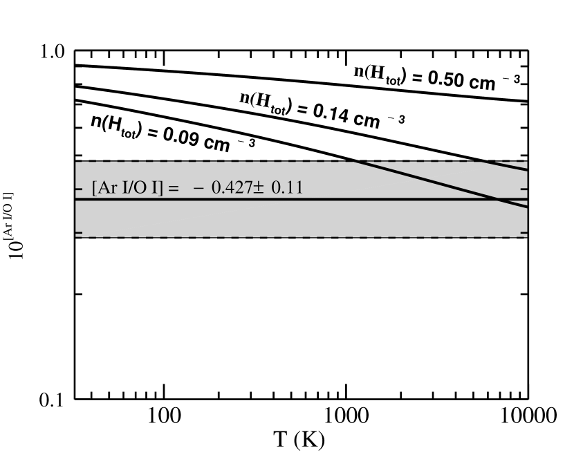
Figure 7: Calculated values for $10^{\rm[ArI/OI]}$ for three different densities $n({\rm H}_{\rm tot})$ and a range of different gas temperatures $T$ shown on the $x$ axis, computed using estimates for the ionization rates from known sources of radiation, both external and internal. A general value for $10^{\rm[ArI/OI]}$ that arose from the survey is indicated by the horizontal line, and the shaded band shows the range of possible systematic errors.

Table 4: Gas Properties

	Without SNR	With SNR	Greater Low
Quantity	Contrib.	Contrib.	Energy Penetration
(1)	(2)	(3)	(4)
$P_{\rm Ar}$	13.1	19.3	12.6
$P^{\prime}_{\rm Ar}$	13.4	22.8	15.9
$n(e)\,({\rm cm}^{-3})$	0.018	0.033	0.052
$n({\rm H}^{0})\,({\rm cm}^{-3})$	0.48	0.48	0.46
$n({\rm H}^{+})\,({\rm cm}^{-3})$	0.015	0.025	0.036
$n({\rm He}^{0})\,({\rm cm}^{-3})$	0.047	0.042	0.035
$n({\rm He}^{+})\,({\rm cm}^{-3})$	3.0e-03	8.1e-03	0.014
$n({\rm He}^{++})\,({\rm cm}^{-3})$	2.1e-05	2.1e-04	1.0e-03
Total $\Gamma({\rm H}^{0})\,({\rm s}^{-1})$	3.2e-16	9.2e-16	2.1e-15
$\ell_{c}$ ($10^{-27}{\rm erg~{}s}^{-1}{\rm H~{}atom}^{-1})$	4.3	6.2	8.5

7.5 Dependence of Recombination with Time

An argument that helps to support the concept that the internal sources spread their ionization rather evenly throughout the medium is that they move at a rate that makes their local residence time short compared to a characteristic $e$-folding time $t_{\rm recomb.}$ for the decay of the proton density from an initial high value to some end equilibrium state $n({\rm H}^{+})_{\rm eq.}$ as $t\rightarrow\infty$,

$$t_{\rm recomb.}=-{n({\rm H}^{+})-n({\rm H}^{+})_{\rm eq.}\over dn({\rm H}^{+})/dt}~{},$$ (23)

where

$$dn({\rm H}^{+})/dt=-\Big{[}\alpha({\rm H}^{0},T)n(e)$$ (24)

$$+ \alpha_{g}({\rm H}^{0},n(e),G,T)n({\rm H_{tot}})$$

$$+ \Gamma({\rm H^{0}})\Big{]}n({\rm H}^{+})+\Gamma({\rm H}^{0})n({\rm H_{tot}})~{}.$$

This expression overlooks the complications arising from charge exchange reactions, and when we evaluate the trend of $n({\rm H}^{+})$ with time we assume that $n(e)$ is always equal to $1.2n({\rm H}^{+})$, as is the case when the gas is in a steady-state ionization condition. Another simplification is that $T$, and hence $\alpha({\rm H}^{0},T)$, remains constant. When the gas is highly ionized, $\Gamma({\rm H}^{0})$ is not equal to the value that we computed for $n({\rm H}^{+})_{\rm eq.}=0.015\,{\rm cm}^{-3}$ because the secondary ionization processes change with $n(e)$ and depend on the strength of the helium ionization. However, we can ignore this complication that occurs at early times because the recombination terms in Eq. 24 are considerably larger than the terms involving $\Gamma({\rm H}^{0})$. The ionization rate influences the character of the decay only when the gas is weakly ionized. Hence there is no harm in declaring that at all times $\Gamma({\rm H}^{0})=3.23\times 10^{-16}{\rm s}^{-1}$, as stated in Table 3. We can adopt for the final state (equilibrium) densities the values $n({\rm H}^{+})_{\rm eq.}=0.015\,{\rm cm}^{-3}$ and $n(e)_{\rm eq.}=0.018\,{\rm cm}^{-3}$ listed in Column (2) of Table 4.

The change of $t_{\rm recomb.}$ with time and the relaxation of $n({\rm H}^{+})$ from a fully ionized condition to $n({\rm H}^{+})_{\rm eq.}$ for $n({\rm H_{tot}})=0.50\,{\rm cm}^{-3}$ and $T=7000\,$K is illustrated in Fig. 8. Values for $t_{\rm recomb.}$ start at 0.13 Myr for an initial $n({\rm H}^{+})=0.50\,{\rm cm}^{-3}$ and increase to 1.0 Myr when $n({\rm H}^{+})$ reaches $0.036\,{\rm cm}^{-3}$ at $t=1.77\,$Myr, beyond which $t_{\rm recomb.}$ very gradually climbs toward a steady value of 1.68 Myr and the subsequent decay in $n({\rm H}^{+})$ toward $n({\rm H}^{+})_{\rm eq.}=0.015\,{\rm cm}^{-3}$ is almost purely exponential.

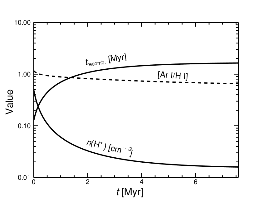
Figure 8: The behavior of $t_{\rm recomb.}$ (upper solid curve) and $n({\rm H}+)$ (lower solid curve) with time $t$, starting from a fully ionized condition to an equilibrium state $n({\rm H}+)_{\rm eq.}$ for $n({\rm H_{tot}})=0.50\,{\rm cm}^{-3}$ and $T=7000\,$K. Values of $t_{\rm recomb.}$ are defined by Eq. 23, and $n({\rm H}+)$ as a function of $t$ can be found by solving the differential equation for $dn({\rm H}+)/dt$ given in Eq. 24. By solving a similar equation for Ar⁺ and comparing it to that for H⁺, we obtain the trend for [Ar I/H I] shown by the dashed line.

Of the three different classes of internal sources, WD stars emit the softest radiation, which means the influences of their ionizations can be more sharply bounded than those of the others. While this consideration may present a challenge to our assumption about the uniformity of ionization in space, we note that these stars have observed radial velocity dispersions of about $25\,{\rm km~{}s}^{-1}$ (Falcon et al. 2010), or rms speeds of $43\,{\rm km~{}s}^{-1}$, which are consistent with the transverse velocity dispersion measurements reported by Wegg & Phinney (2012). This indicates that WDs typically move about 76 pc during the time interval that $n({\rm H}^{+})$ decays from 0.50 to $0.036\,{\rm cm}^{-3}$. This amount of travel is considerably larger than the radius of a Strömgren Sphere

$$r_{\rm S}=\left({3r^{2}_{*}\int_{13.6\,{\rm eV}}^{\infty}F(E)_{\rm WD}dE\over n({\rm H})^{2}\alpha({\rm H}^{0},T)}\right)^{1/3}$$ (25)

that would be established if a WD star were stationary. (Recall that $F(E)_{\rm WD}$ is the flux emitted at the surface of the star with a radius $r_{*}$.) A typical value for $r_{\rm S}$ in the WNM would be about 1.8 pc; this value applies to a WD star with $r_{*}=0.014r_{\odot}$ that has $T_{\rm eff}=50,000\,$K and is situated within a gas with a density $n({\rm H_{tot}})=0.50\,{\rm cm}^{-3}$.

One can view the dispersal of ionization caused by the star’s motion in the context of the simplified description of “cometary H II regions” described by Raga (1986); the dimensionless elongation parameter in this development $\beta=3v/[n({\rm H_{tot}})\alpha({\rm H}^{0},T)r_{\rm S}]=14$ if $r_{\rm S}=1.8\,$pc and $v=43\,{\rm km~{}s}^{-1}$, which would result in a tube of ionization with a radius $\sim 0.5r_{\rm S}$ and a very long tail. The fact that the ionizations produced by WD stars could be highly diluted because they are distributed over large volumes could explain why a sensitive survey of H$\alpha$ emission from regions around such stars carried out by Reynolds (1987) yielded only one detection out of nine targeted regions surrounding these stars.

8 PROPOSALS FOR ADDITIONAL PHOTOIONIZATION

Given that the outcome for a reasonable value of $n({\rm H}_{\rm tot})$ and the ionization rate from known sources discussed in Section 7 do not agree with our observations, we must explore some alternatives for boosting the average rate of photoionization in the WNM. Two possibilities are discussed in the following sections.

8.1 Ionization from Previous Supernova Remnants

A popular theme in the ISM literature of early 1970’s was the consideration that the low density portions of the ISM were ionized impulsively by UV and X-ray radiation from supernovae and their remnants (SNRs), which represented sources of ionization that had limited durations and that materialized at random locations and times (Bottcher et al. 1970; Werner et al. 1970; Jura & Dalgarno 1972; Gerola et al. 1973; Schwarz 1973). A particularly instructive example that shows the wide variations in temperature and fractional ionization can be seen in the results from a numerical simulation by Gerola et al. (1974). This topic has also been approached by Slavin et al. (2000), who estimated the effects of irradiation of the neutral medium by SNRs, with a special emphasis on its influence on gas in the Galactic halo. The spectral character and strength of the emitted radiation from a remnant depends on a combination of supernova energy and the density of the ambient medium (Mansfield & Salpeter 1974). The emission of soft X-rays as a remnant evolves can last up to a late phase when radiative cooling causes a dense shell to form, which could be opaque to the lowest energy X-rays. However some of the radiation may continue to escape afterward if instabilities cause the shell to break up and create gaps (Vishniac 1994; Blondin et al. 1998). The magnitudes of such instabilities are uncertain, since they might be diminished if either the ambient medium has a low density and high temperature (Mac Low & Norman 1993) or if the shock is partly stabilized by an embedded transverse magnetic field (Tóth & Draine 1993).

Chevalier (1974) has computed the strength and distribution over energy for the radiation emitted by various models for SNRs. As a representative example, we can use the emission over a time interval of $2.5\times 10^{5}\,{\rm yr}$ from his model that had an energy $E_{\rm SN}=3\times 10^{50}\,{\rm erg}$ and was expanding into a medium with an average density of $1\,{\rm cm}^{-3}$. If we assume that there was a succession of about 3 such remnants that occurred once every Myr (i.e., of order $t_{\rm recomb.}$ defined in Eq. 23 for $n({\rm H}^{+})=0.036\,{\rm cm}^{-3}$; see Fig. 8) and they were at a distance of 100 pc from some location in the ISM, the resulting time-averaged flux shown by the dashed line in the upper panel of Fig. 6 would increase the total ionization of H from $\Gamma({\rm H}^{0})=3.2\times 10^{-16}{\rm s}^{-1}$ for the steady ionization sources to the much higher value of $9.2\times 10^{-16}{\rm s}^{-1}$ and create conditions that would yield values for [Ar I/O I] that are virtually the same as those depicted by the curve labeled $n({\rm H}_{\rm tot})=0.14\,{\rm cm}^{-3}$ in Fig. 7, but in this case for a density $n({\rm H}_{\rm tot})=0.50\,{\rm cm}^{-3}$. At $T=7000\,$K, the densities of various constituents are represented by the numbers that are shown in Column (3) of Table 4. For this temperature, the calculation of [Ar I/O I] is just consistent with the upper error bound from the observations.

A stronger flux from SNRs would be needed to make the calculated value for [Ar I/O I] match nominal value for the observed ones. To obtain a curve that matches the lowest curve (labeled $n({\rm H}_{\rm tot})=0.09\,{\rm cm}^{-3}$) in Fig. 7 and still maintain an assumed local density $n({\rm H}_{\rm tot})=0.50\,{\rm cm}^{-3}$, we would require either an increase in the average energy of the supernovae (SNe), or the rate would need to be increased from 3 to 8 SN ${\rm Myr}^{-1}$ at a distance of 100 pc. In this circumstance, $n(e)=0.047\,{\rm cm}^{-3}$.

While one might be tempted to ask whether some average SN rate in our location within the Galaxy (van den Bergh & McClure 1994; McKee & Williams 1997; Ferrière 2001) is consistent with at least 3 SNe Myr^-1 at separations of about 100 pc from some representative location, it is probably more realistic to draw upon actual estimates of the recent history of explosions in the general neighborhood of the Sun, which have been inspired by the evidence of how the ISM has been disrupted by the expansions of the explosion remnants. The Local Bubble (see footnote 2 in Section 2) and the neighboring radio emitting Loop I superbubble, which intersect one another (Egger & Aschenbach 1995), are both thought to have been created by a series of SN explosions that occurred over the past 10-15 Myr (Maíz-Apellániz 2001; Berghöfer & Breitschwerdt 2002). Fuchs et al. (2006) analyzed the numbers and mass functions of stars within nearby O-B associations and traced their motions back in time. From this information, they concluded that the Local Bubble was created by 14-20 SNe. This estimate is consistent with the 19 SNe that Breitschwerdt & de Avillez (2006) used in their hydrodynamic simulation of the creation of the Local Bubble.

Within a shorter time frame, there is some evidence that atoms from a nearby SN were deposited on the Earth some 2.8 Myr ago, as revealed by an enhancement of ⁵⁶Fe in a thin layer within deep-sea ferromanganese crust (Knie et al. 2004). Fitoussi et al. (2008) attempted to replicate this result in a marine sediment, but the outcome did not agree with the earlier result at the same level of significance. However, there are alternative means for investigating past depositions of SN elements in terrestrial samples (Bishop & Egli 2011; Feige et al. 2012), and new results may emerge soon.

If we add to the Local Bubble contribution the past SNe in the Sco-Cen association that created Loop I (Iwan 1980; Egger 1998; Diehl et al. 2010), one can imagine that, to within the uncertainties in the X-ray production rates, the time-averaged level of ionizing radiation could conceivably be of the same order of magnitude as that discussed in the preceding paragraphs.

A legitimate question to pose is whether or not, at some intermediate stage of recombination, the value of [Ar I/H I] makes a brief excursion to a level below the final equilibrium state. If this were the case, we might be able to relax the requirement for a high frequency of SN explosions. The recombination rates $\alpha({\rm H}^{0},T)$ and $\alpha({\rm Ar}^{0})$ are nearly equal to each other, but the dust grain recombination rate $\alpha_{g}$ for Ar should be much less than that for H because the thermal velocities of Ar are lower. Thus, at early times where recombinations still dominate over the steady-state ionization rate but the electron density has decreased to a point that neutralization of Ar and H by collisions with dust grains become important, one could imagine that the difference in grain recombination rates might be influential in allowing the H⁺ to recombine more quickly than Ar⁺. In order to investigate this possibility, we can evaluate the time history of the Ar recombination using Eqs. 23 and 24 but with a substitution of “Ar” for each appearance of “H.” A resulting comparison of the Ar recombinations to those of H shows that [Ar I/H I] shows a steady decrease from an initial value slightly greater than 1.0 (when the gas is just starting to recombine) to the final equilibrium state for this quantity without any excursion to lower values. This behavior is illustrated by the dashed line in Fig. 8.

8.2 Penetration of the WNM by Low-energy Photons

Until now, we have regarded the emission of X-rays from the hot ($T\sim 10^{6}\,$K) gas in our Galaxy as an external source of ionizing radiation that must penetrate the bulk of the WNM regions under study. With this condition in mind, we established a 90 eV cutoff for the external radiation, below which the X-rays were assumed to be absorbed in the outer layers of the neutral gas. However, some of the soft X-ray emitting gas may be threaded through the WNM, a picture that is reminiscent of the network of hot interstellar tunnels proposed by Cox & Smith (1974). Hot, interspersed gas could allow some or all of the neutral medium to have access to lower energy radiation. Observations indicate that O VI, an indicator of gas that is collisionally ionized at $T\sim 3\times 10^{5}\,$K, can be seen in emission (Dixon et al. 2006; Otte & Dixon 2006) and absorption (Jenkins 1978a, b; Bowen et al. 2008) almost everywhere in the disk of the Galaxy. The simulations of SNe exploding at random in the Galactic disk by Ferrière (1995) and de Avillez & Breitschwerdt (2005a, b) indicate that this hot gas should be sufficiently pervasive and frothy that, even though our measurements penetrate through column densities well in excess of $10^{19}\,{\rm cm}^{-3}$, individual parcels of gas may be exposed to adjacent sources of radiation through significantly lower column densities. Indeed, there could be unusually strong X-ray emission at the boundaries where the neutral regions come into contact with the hot gas, where charge exchange reactions between neutrals and highly ionized species could produce an enhancement of soft X-ray emission over that which is emitted by just the hot gas (Wang & Liu 2012).

It is clear from the gray parts of the external radiation spectrum depicted in Fig. 6 that even a modest lowering of the cutoff below our adopted 90 eV threshold will create a significant increase in the ionization of the WNM. For instance, if the threshold were dropped to 60 eV, an energy just below the strong M-line complex of emission features from highly ionized Fe at 70 eV, the level of ionization would increase to an extraordinarily large total hydrogen ionization rate $\Gamma({\rm H}^{0})=2.1\times 10^{-15}{\rm s}^{-1}$. For $n({\rm H}_{\rm tot})=0.50\,{\rm cm}^{-3}$ and $T=7000\,$K, this increase would create a value for [Ar I/O I] that is consistent with the upper error bound for the measured outcomes. In this particular case, most of the ionization is caused by photons with energies near 70 eV. For this energy, $P_{\rm Ar}(E)$ is near its minimum value (see the lower panel of Fig. 5 and the entry in Column (4) of Table 4). As a consequence, in order to match our observations, Eq. 7 shows us that the required $n({\rm H}^{+})$ (and thus $\Gamma({\rm H}^{0})$) must be increased beyond the value needed from the time-averaged SNR radiation with its larger value of $P_{\rm Ar}$.

A consideration that disfavors the presence of a strong ionizing flux at energies in the vicinity of 70 eV, at least at our location, is that it does not seem to be present at anywhere near the intensity level shown in Fig. 6. For instance, from observations by the Cosmic Hot Interstellar Plasma Spectrometer (CHIPS) Hurwitz et al. (2005) stated an upper limit for the flux emitted by the Fe lines near 70 eV. This limit was consistent with an emission measure for a plasma with a solar abundance pattern at $T=10^{6}\,$K that is less than 5% of the value ${\rm EM}=10^{16.37}{\rm cm}^{-5}$ that we used for reconstructing the emission spectrum from the soft component of the X-ray background described in Section 7.1. Jelinsky et al. (1995) and Bloch et al. (2002) similarly found flux upper limits at low energies (but not as stringent as those from CHIPS) that were much lower than model predictions at this energy that we obtained from fits to the observed radiation at higher energies. A marginal detection of the Fe emission complex toward high Galactic latitudes by McCammon et al. (2002), $F(E)=100\pm 50\,{\rm phot~{}cm}^{-2}{\rm s}^{-1}{\rm sr}^{-1}$ is also well below the peak at 70 eV that appears in our reconstructed flux. The weakness of these fluxes could be caused either by a deficiency of Fe below the solar abundance ratio in the hot emitting gases or by our inability to see hot gas regions whose low energy radiation is not absorbed by intervening neutral material.

9 DISCUSSION

We have now reached a point where it is appropriate to investigate the consistency of the newly derived WNM ionization levels with other observational and theoretical findings, along with some consequences of our results on various relevant physical processes.

9.1 Other UV Observations

Along a number of sight lines, there have been detailed investigations of UV absorption lines observed at high enough velocity resolutions to identify which components came from either mostly neutral or mostly ionized clouds (Spitzer & Fitzpatrick 1993, 1995; Fitzpatrick & Spitzer 1994, 1997; Wood & Linsky 1997; Holberg et al. 1999; Welty et al. 1999; Jenkins et al. 2000a; Gry & Jenkins 2001; Sonnentrucker et al. 2002). These investigations relied either on the relative populations of the excited fine-structure level of ${\rm C}^{+}$ or the ratios of ions to neutrals for various elements. The ion-to-neutral ratios of different elements gave very different outcomes for $n(e)$ (but systematically went up and down together from one velocity component to the next); these disparities probably arose as a result of a lack of a good understanding of the physical processes involved. Welty et al. (2003) have presented a good summary of the results that exhibited this problem.

Values of $n(e)$ identified with the WNM by the investigators cited above generally ranged between 0.04 and $0.12\,{\rm cm}^{-3}$, which seem to be higher than our values given in Table 4. A common theme in the discussions of these results was that such high partial ionizations could not be attributed to the known EUV, X-ray and cosmic ray ionization rates – a conclusion that is stated once again from our [Ar I/O I] results.

Electron densities for clouds embedded in the Local Bubble have an average value of $0.11\,{\rm cm}^{-3}$ (Redfield & Falcon 2008), a result that once again relied on comparisons of excited C⁺ to other species (either unexcited C⁺ or S⁺). The fractional ionization of these clouds appears to be much higher than what we found for the general WNM outside the Local Bubble, if one assumes that the characteristic total density $n({\rm H}_{\rm tot})\approx 0.2\,{\rm cm}^{-3}$ within the clouds (Redfield & Linsky 2008). By solving for the time-dependent ionization in Eq. 24 for $n({\rm H_{tot}})=0.2\,{\rm cm}^{-3}$, we find that the decay from a fully ionized condition to an approximately half ionized state takes only 0.40 Myr. It is likely that this higher level of ionization might be explained by supplemental radiation from evaporative boundaries that surround the clouds (Slavin & Frisch 2002), if indeed they are embedded in a very hot, low density gas, or by the infiltration of some ionizing radiation from $\epsilon$ CMa, which strongly dominates over other radiation sources within the Local Bubble at low energies (Vallerga & Welsh 1995).

9.2 Pulsar Dispersion Measures

Cordes & Lazio (2002) have derived characteristic electron densities for three volumes within about 1 kpc of the Sun. Inside the Local Bubble, their model seems to best fit an average density of only $\langle n(e)\rangle=0.005\,{\rm cm}^{-3}$, which is not surprising because much of the volume has probably been cleared of material by SN explosions, except for some isolated, warm clouds with an average filling factor in the range $5.5-19$% (Redfield & Linsky 2008). Regions outside the Local Bubble have higher densities: two volumes that they studied yield $\langle n(e)\rangle=0.012$ and $0.016\,{\rm cm}^{-3}$. However, these regions are identified with ellipsoidal volumes designated as either a “local superbubble” (LSB) or a “low density region” (LDR), so they too could have significant voids that would dilute the apparent electron densities. The values of $\langle n(e)\rangle$ given for these regions could be consistent with our measures of $n(e)$ given in the last two columns of Table 4 for the WNM if this medium had a filling factor of about 1/3 in these regions and there were no significant contributions from the warm ionized medium (WIM).

An independent analysis of dispersion measures was carried out by de Avillez et al. (2012) for 24 pulsars with known distances between 0.2 and 8 kpc from the Sun and with $|z|<0.2\,$kpc. They found a distribution of $n(e)$ outcomes that was consistent with a log-normal distribution centered on $\log n(e)=-1.47$ and a dispersion $\sigma[\log n(e)]=0.17$. The fact that their representative values of $n(e)$ are higher than the determination of Cordes & Lazio (2002) and close to our findings based on [Ar I/O I] may be accidental, since their results may be strongly influenced by sight-line interceptions of fully ionized regions.

9.3 Emission Lines

Observations of diffuse line emissions in the sky most generally apply to probing the physical conditions in fully ionized gases, either the bright H II regions around hot stars or the WIM (Reynolds et al. 1977, 2002; Haffner et al. 1999; Madsen et al. 2006). Most of the emissions are dominated by contributions from species that are expected to be abundant in such highly ionized media, and they should overwhelm any contributions from the very dilute ionization in the WNM. Nevertheless, there are a few cases where emission line fluxes from some neutral species in the WIM are expected to be very weak, and thus a contribution from the WNM might in principle be identified. We need to explore whether or not the predictions for line strengths from a medium with our enhanced electron densities are not in serious violation of detections or the upper limits for the fluxes. We explore three such cases in the subsections that follow. The first test involving line emission from He recombinations is especially important, because we predict that the fraction of singly-ionized He could be as high as 16$-$28% of the total amount of helium.

9.3.1 He $\lambda$5876 Recombination Radiation

Reynolds & Tufte (1995) attempted to compare the strength of the recombination line of He⁰ at 5876 Å to that of H$\alpha$ in parts of the sky away from well defined H II regions. Their motive was to determine the hardness of the radiation that maintains the ionization in the WIM. While an explicit upper limit for the He recombination line flux was not stated by Reynolds & Tufte (1995), we estimate that the flux in the two directions that they sampled was found to be less than 0.1 R (R = Rayleigh = $10^{6}/(4\pi){\rm phot~{}cm}^{-2}{\rm sr}^{-1}{\rm s}^{-1}$).

Using the line emission rates given by Benjamin et al. (1999) we find that for $n(e)=0.04\,{\rm cm}^{-3}$, $n({\rm He}^{+})=0.01\,{\rm cm}^{-3}$, and $T=7000\,$K (representative values for the enhanced ionization cases presented in the last two columns of Table 4) the emission should be $3.0\times 10^{-17}{\rm phot~{}cm}^{-3}{\rm s}^{-1}$. If we were to propose that the emission is seen over a path of 200 pc with no extinction (i.e., imagine a length of 400 pc with a filling factor for the WNM of 50%), we could expect to find an emission of $1500\,{\rm phot~{}cm}^{-2}{\rm sr}^{-1}{\rm s}^{-1}=0.02\,$R. This expectation is well below the sensitivity of the observations by Reynolds & Tufte (1995), so our predicted intensity from the enhanced electron density and ionization of He does not violate their upper limit.

9.3.2 Emission of [O I] $\lambda$6300 from Electron Collisions

In order to determine the neutral fraction of H in the WIM, Reynolds et al. (1998) measured the strength of the [O I] $\lambda$6300 line emitted in parts of the sky that had a uniform, moderately strong H$\alpha$ emission (but away from obvious H II regions excited by stars), much as they had done for the He recombination line discussed above. In three different directions, they detected intensities of 0.2, 0.09, and 0.11 R.

According to Federman & Shipsey (1983), electron collisions dominate over those by hydrogen for the excitation of the ${}^{1}D_{2}$ state of neutral oxygen when the electron fraction exceeds $1.5\times 10^{-4}$. Hence, we can ignore hydrogen impacts. From the fitting formula of Péquignot (1990) to the collision strengths computed by Berrington & Burke (1981), we derive a collisional rate constant $C_{e}$ for electron excitations to be $8.0\times 10^{-11}{\rm cm}^{3}{\rm s}^{-1}$ at $T=7000\,$K. If we again make the conservative assumption expressed in Section 4.2.1 that at the low densities of the WNM the depletion of O is negligible, we expect that $n({\rm O}^{0})=2.7\times 10^{-4}{\rm cm}^{-3}$ if $n({\rm H}^{0})=0.47\,{\rm cm}^{-3}$. For $n(e)=0.04\,{\rm cm}^{-3}$, we expect the emissivity to be equal to $n({\rm O}^{0})n(e)C_{e}$ multiplied by a branching fraction 0.76 (Froese Fischer & Tachiev 2010) for the proportion of decays from the ${}^{1}D_{2}$ level to the lower ${}^{3}P_{2}$ level. This product equals $6.6\times 10^{-16}{\rm phot~{}cm}^{-3}{\rm s}^{-1}$, which should produce 0.41 R over a path of 200 pc. This value is greater than the three measurements by Reynolds et al. (1998). The magnitude of this violation is not large, considering the uncertainties of our assumptions about the lack of depletion of O and the adopted path length estimate. Also, for temperatures less than 7000 K, the expected strength of the emission will be considerably less: for instance, at $T=5000\,$K, the emission should be 4.5 times weaker than at 7000 K.

9.3.3 Emission of [N I] $\lambda$5201 from Electron Collisions

An upper limit of 0.13 R for the [N I] $\lambda$5201 line was determined for a single direction in the sky by Reynolds et al. (1977). If we adopt the same calculations as in the previous section for O I, but make the substitution that $n({\rm N}^{0})=8.0\times 10^{-5}n({\rm H}^{0})=3.8\times 10^{-5}{\rm cm}^{-3}$ (again, assuming no depletion), and $C_{e}=8.6\times 10^{-11}{\rm cm}^{3}{\rm s}^{-1}$ at $T=7000\,$K (Tayal 2006), we obtain an emissivity equal to $1.3\times 10^{-16}{\rm phot~{}cm}^{-3}{\rm s}^{-1}$, which yields an intensity of 0.08 R over a 200 pc path. This value is below the upper limit determined by Reynolds et al. (1977).

9.4 Cooling Rates from Carbon Ions and Oxygen Atoms

A major coolant for the neutral ISM is the singly charged carbon ion (Dalgarno & McCray 1972; Wolfire et al. 1995, 2003), whose ${}^{2}P_{3/2}$ excited fine-structure level in the ground electronic state can be excited by collisions with electrons and hydrogen atoms. The cross section for excitation by electrons is substantially greater than that for neutral hydrogen. For this reason, the level of partial ionization is an important factor in the excitation rate. After excitation, an energy loss can occur because the excited level can undergo a spontaneous radiative decay with a transition probability $A_{21}=2.29\times 10^{-6}{\rm s}^{-1}$ to the lower ${}^{2}P_{1/2}$ state (Nussbaumer & Storey 1981), a process that liberates a photon with a wavelength of $158\,\mu$m. If we assume that the abundance ratio $({\rm C}^{+}/{\rm H}^{0})=9.5\times 10^{-5}$ (see footnote 1 in Section 1), we can use the densities that we derived for $n({\rm H}^{0})$ and $n(e)$ along with the excitation cross section by H⁰ impacts computed by Barinovs et al. (2005) and electron collision strengths of Wilson & Bell (2002) to compute the ${\rm C}^{+*}$ energy loss rates $\ell_{c}$ per H atom. These rates are given in the last row of Table 4. They do not change in direct proportion to $x_{e}$ because about half of the excitations come from collisions with H atoms, which are more numerous than the electrons. In addition, the overall cooling rate for the WNM does not increase in direct proportion to $\ell_{c}$ because it accounts for only about one-third of the total cooling.

Most of the remaining cooling comes from the fine-structure excitation of O I and the subsequent emissions at 44 and $63\,\mu$m. The O I cooling is insensitive to changes in $x_{e}$ because the collision rate constants for electrons (Bell et al. 1998) are much less than those for neutral hydrogen. Using an extrapolation of the atomic hydrogen collisional rate constants given by Abrahamsson et al. (2007) above a temperature of $10^{3}\,$K, the spontaneous decay rates of the two excited levels given by Galavís et al. (1997), and ${\rm O/H}=5.75\times 10^{-4}$, we find that for $n({\rm H}^{0})=0.47\,{\rm cm}^{-3}$ and $T=7000\,$K that the energy loss rate per H atom $\ell_{o}=1.13\times 10^{-26}{\rm erg~{}s}^{-1}$.

The results for $\ell_{c}$ shown in the table are significantly lower than the average value of $2\times 10^{-26}{\rm erg~{}s}^{-1}{\rm H~{}atom}^{-1}$ found for low-velocity clouds by Lehner et al. (2004), who measured the column densities of C II^∗ from spectra recorded by FUSE. [Lehner et al. (2003) obtained similar results for sight lines toward WD stars within or just outside the Local Bubble.] Lehner et al. (2004) compared their results with measurements of H$\alpha$ emission in the same directions, and they concluded that about half of the C II^∗ that they detected came from fully ionized gas (but with large variations from one sight line to the next). This inference was supported by the fact that their values of $\ell_{c}$ were slightly lower for sight lines with large values of $N$(H I). In principle, one can gain an insight on the relative importance of H II regions by comparing the observed abundances of C^+∗ to those of N^+∗, since the former can come from both neutral and ionized regions, while the latter arises only from ionized regions. Gry et al. (1992) compared these two species in a comprehensive study of both the absorption lines observed by the Copernicus satellite (Rogerson et al. 1973) and the 158 and 205$\mu$m emission lines observed by the COBE satellite (Wright et al. 1991). They concluded that H II regions were responsible for a major portion of the C^+∗ that was observed, but this result is clearly dependent on the assumed ratio of atomic C to N in the H II regions.

An important advantage of the $\ell_{c}$ determinations synthesized from our results for [Ar I/O I] is that they apply only to the WNM; hence they give more accurate indications of the carbon cooling rates within this medium without any contamination from H II regions. They do, of course, rely on the value of assumed relative abundances of C and H in the gas phase.

9.5 Heating Rates

9.5.1 Thermal Time Constants

The cooling time for a medium with $T=7000\,$K and thermal pressure $nT=3800\,{\rm cm}^{-3}$K (Jenkins & Tripp 2011) is about 4.1 Myr [ (Wolfire et al. 2003); see their Eq. (4)]. However, when the medium is impulsively heated and ionized by the EUV and X-ray illuminations from a SNR, the temperature can approach or exceed $10^{4}\,$K, and the onset of L$\alpha$ cooling creates a dramatic increase in the overall cooling rate (Dalgarno & McCray 1972). When this happens, the thermal relaxation timescale becomes much shorter than the mean interval between the bursts of radiation, each of which last only about one to a few times $10^{5}\,$yr. Thus, while we can compute a time-averaged heating rate for the SNR illuminations that might explain our high levels of partial ionization, we have no reason to expect that this average should be balanced by the cooling rates that would apply for the medium at $T=7000\,$K.

9.5.2 Secondary Electrons

The same energetic electrons that are responsible for the secondary ionizations $\Gamma_{s}$ and $\Gamma_{s^{\prime}}$ can also heat the gas through collisions with other electrons. As with the calculations of the efficiency of secondary ionizations described in Appendix A, we use the analytic approximations of Ricotti et al. (2002) for the heating efficiencies, based on the numerical results for various conditions obtained by Shull & Van Steenberg (1985). Aside from replacing ionization efficiencies with heating efficiencies and multiplying by the energies of the respective secondary electrons, the calculations here are virtually the same as for the ionization rates.

Table 5 shows the outcomes for the evaluations of secondary electron heating rates. It is no surprise that there is a substantial increase in the heating rates when we advance from the ionization created by known sources to either of the two hypothetical enhanced ionization examples that could explain the electron fractions indicated by the observations of [Ar I/O I].

Our high result ($1.2\times 10^{-25}{\rm erg~{}s}^{-1}{\rm H~{}atom}^{-1}$) for the heating in the regime where there is increased penetration of X-rays down to 60 eV creates a serious problem for this model, since this steady-state rate is considerably larger than the corresponding cooling rate $\ell_{c}+\ell_{o}=1.98\times 10^{-26}\,{\rm erg~{}s}^{-1}{\rm H~{}atom}^{-1}$ given in Section 9.4.

9.5.3 Cosmic Ray Heating of Electrons

In addition to ionizing the gas and creating secondary electrons that can heat the gas, cosmic rays can also interact with free electrons in the medium and heat them. The heating rate per unit volume is approximately equal to $A\zeta_{\rm CR}({\rm H}^{0})n(e)$, where $A\approx 4.6\times 10^{-10}{\rm erg}$ (Draine 2011, p. 338). With the electron densities listed in Table 4 and $\zeta_{\rm CR}=1.25\times 10^{-16}{\rm s}^{-1}{\rm H~{}atom}^{-1}$, we find that for the three different electron densities in this table the heating rates are $1.0\times 10^{-27}$ (for no SNR contribution), $1.9\times 10^{-27}$ (with SNR contributions), and $3.0\times 10^{-27}{\rm erg~{}cm}^{-3}{\rm s}^{-1}$ (for the lower energy penetration example). After dividing these numbers by values of $n({\rm H}^{0})$ given in Table 4, we find that these rates are about 0.4 to 1.2 times the rate from secondary electrons liberated by the cosmic rays, and 0.05 to 0.5 times the respective heating rates from the secondary electrons generated by ionizations from the X-ray backgrounds.

Table 5: Secondary Electron Heating Rates

	Rate
Source	($10^{-27}{\rm erg~{}s}^{-1}\,{\rm H~{}atom}^{-1}$)
X-ray background (no SNR)	4.1
X-ray background (plus SNR)	50
X-ray background (down to 60 eV)	110
Main-sequence stars	1.5
Active binaries	0.063
WDs	0.84
Cosmic rays	4.9
He+ recomb. (background with no SNR)	0.059
He+ recomb. (background plus SNR)	1.2
He+ recomb. (background down to 60 eV)	8.8

Table 6: Dust Grain Heating and Cooling Rates

	Without SNR				With SNR				Greater Low
$b_{c}$	Contrib.				Contrib.				Energy Penetration
$\times 10^{5}$	H	C	$\Delta$		H	C	$\Delta$		H	C	$\Delta$
(1)	(2)	(3)	(4)		(5)	(6)	(7)		(8)	(9)	(10)
0.0	9.9	5.1	4.8		16.1	7.5	8.5		22.0	10.0	12.0
2.0	15.1	7.3	7.8		23.2	11.0	12.1		30.7	14.9	15.8
4.0	24.4	10.6	13.9		36.4	16.0	20.4		46.9	21.8	25.1
6.0	31.6	13.8	17.8		47.4	20.9	26.5		61.3	28.5	32.9

9.6 Dust Grains: Photoelectric Heating and Recombination Cooling

When dust grains are illuminated by starlight, they emit photoelectrons, which can heat the medium (Watson 1972; Draine 1978; Pottasch et al. 1979; Bakes & Tielens 1994; Weingartner & Draine 2001b). This heating is partly offset by collisional cooling via grain-ion recombination (Draine & Sutin 1987). The efficiencies of these mechanisms are regulated by the charge of the grains, which in turn depends on $n(e)$, $T$ and $G$ (the density of starlight). Table 6 shows our calculations of grain heating and cooling for the three cases (no SNR, with SNR, and lower energy X-ray penetration) using the fitting formulae and coefficients given by Weingartner & Draine (2001b); see note $a$ of the table for details.

It is generally regarded that the photoelectric heating from grains is greater than that from cosmic rays by about one order of magnitude (Draine 2011, p. 339) [or considerably more than this if the assumed value for $\zeta_{\rm CR}({\rm H}^{0})$ is lower than that adopted here, e.g., Wolfire et al. (1995, 2003)]. Any enhancement in $x_{e}$ tends to increase the heating rate from grains, since the grains will be more negatively charged. However, this increase is not as strong as the effect of a greater electron fraction on the direct cosmic ray heating, so the disparity between the two rates is decreased.

10 SUMMARY AND CONCLUSIONS

We have developed a means for deriving the representative rates of ionization, and thus the resulting electron densities, along sight lines that penetrate the WNM and that extend out to several hundred pc from us, well beyond the edge of the Local Bubble. Our method makes use of the fact that when a mostly neutral medium is exposed to the ambient EUV and soft X-ray ionizing radiation, the argon atoms are far more susceptible to being ionized than hydrogen atoms. Thus, by comparing the abundances of Ar I to those of H I, we gain an understanding of the strength of the photoionization and secondary processes related to it. For a number of practical reasons, we find that it is desirable to use O I as a proxy for H I. The partial ionization of oxygen is strongly coupled to that of hydrogen through a rapid charge exchange process. Using this strategy, we compare the column densities of Ar I and O I derived from absorption lines seen in the FUSE spectra of 44 hot subdwarf stars.

Since the neutral forms of argon and oxygen are virtually absent in regions that are fully ionized (either the prominent H II regions around hot stars or the much lower density but more pervasive WIM), our probes sample only regions that have appreciable concentrations of H I. This sets our measurements apart from conventional determinations of average electron densities (e.g., pulsar dispersion measures, H$\alpha$ intensities, C II fine-structure excitation, etc.), which are strongly influenced by contributions from the fully ionized regions.

We find that, on average, the abundance of neutral argon, relative to that of neutral oxygen, is $[{\rm Ar~{}I/O~{}I}]=-0.427\pm 0.11\,$dex below what we would expect if both species had no partial ionization and the solar abundance ratio is a proper standard of comparison. We interpret this deficiency in terms of the greater susceptibility of argon to photoionization. After accounting for a broad range of processes that can modify the fractional ionizations, we conclude that with known sources of ionizing radiation, both external and internal, the only straightforward way to reconcile the large deficiency of Ar I is to propose that the neutral medium has a characteristic density of only $0.09\,{\rm cm}^{-3}$, which is far below a generally accepted value of about $0.5\,{\rm cm}^{-3}$. At this latter, higher volume density of hydrogen, known sources of ionization should produce an electron density $n(e)=0.018\,{\rm cm}^{-3}$ and create a result $[{\rm Ar~{}I/O~{}I}]=-0.14$, which is greater than all but a small fraction of the measurements and well above the overall average value.

In order to achieve a result for [Ar I/O I] that is consistent with both our observations and a density $n({\rm H~{}I})=0.5\,{\rm cm}^{-3}$, we must propose nonconventional sources of additional ionization. We discuss two such possibilities; in reality we might be witnessing the outcome of some combination of both of them working together.

The first explanation is that the shielding of the external, low energy X-ray flux is less effective than expected: if we lower the cutoff energy from a nominally expected 90 eV to only 60 eV, we can gain sufficient additional ionizing photons from the external background to create a level of ionization that is consistent with an upper bound for the value implied by our observed [Ar I/O I]. To explain this lower shielding, one might envision a nearly sponge-like topology for the WNM, where the internal holes and channels are filled with hot, X-ray emitting gas. Indeed, de Avillez et al. (2012) have performed hydrodynamical simulations of the effects from random SN explosions and stellar winds in the plane of the Galaxy, and the outcome of their model exhibits a complex, turbulent entanglement of hot, warm and cold gas complexes. Their simulation, which includes non-equilibrium ionization calculations, yields an average electron density $n(e)=0.04\,{\rm cm}^{-3}$, a value that is not far removed from our determination for the WNM. This near match may be coincidental, however. In the simulation, voids containing hot, collisionally ionized gas with very low $n(e)$, in combination with dense regions that are photoionized, may produce an outcome that is close to the value for the WNM.

A serious shortcoming of the interpretation that we are viewing a steady-state maintenance of a high level of ionization in the WNM is that the calculated heating rate of $1.2\times 10^{-25}\,{\rm erg~{}s}^{-1}\,{\rm H~{}atom}^{-1}$ from secondary electrons is unacceptably high – much higher than the cooling rate from atomic fine-structure excitations or recombinations of ions onto dust grains.

Our second explanation is a time-dependent solution that can sidestep the problem of overheating in the equilibrium case discussed above. Over a period of one to a few times $10^{5}\,$yr, an SNR can create a burst of ionizing radiation in the X-ray region that can briefly elevate the ionization of the ISM to levels well above normal out to distances of order a few hundred pc away. Initially, the recombination timescale is quite short, but then it advances to about 1 Myr when the level of ionization approaches our observed average state. For heating by secondary electrons, the temperature should exhibit a similar rapid adjustment that is followed by a much slower trend with time. The radiation burst will indeed create a very high heating rate, but as the gas temperature approaches or exceeds $10^{4}\,$K, the abrupt onset of the very strong L$\alpha$ cooling will dump most of the heat over a time scale that is considerably shorter than the cooling time ($\sim 4\,$Myr) for the gas in its usual state. A good exposition of this quick thermal recovery to $T<10^{4}\,$K and a comparatively more gentle relaxation in the heat loss and recombinations can be seen in plots of $T$ and $x_{e}$ vs. time in Fig. 2 of Gerola et al. (1974).

We propose that the ionization imprint of an SN explosion on the WNM can last well beyond the time that the remnant is recognizable in X-rays. We have good evidence that a number of SNe have exploded in our general vicinity over the past $1-10\,$Myr. As a consequence, if one considers that the activity in our neighborhood has recently been higher than normal for our Galaxy, the WNM out to several hundred pc from the Sun may be ionized to a level that is somewhat higher than the low-density neutral gas at similar galactocentric distances elsewhere in the Galactic plane.

Appendix A IONIZATION BY SECONDARY ELECTRONS $\Gamma_{s}$ AND $\Gamma_{s^{\prime}}$

A.1 Electrons from H and He

In order to determine $\Gamma_{s}({\rm H}^{0})$, [and, later, $\Gamma_{s}({\rm He}^{0})$ and $\Gamma_{s}({\rm Ar}^{0})$], we start by considering the effects from the secondary electrons that are produced by the primary photoionizations of both H and He. To do so, we evaluate various forms of the quantity $\phi({\rm H}^{0},E_{e},x_{e})$, which represent the number of additional ionizations created by the collisions from the photoejected electrons with energy $E_{e}=E-{\rm IP}({\rm H^{0},~{}He^{+},He^{++}})$ and any cascade of additional electrons that may follow. ($E$ is the original photon energy, and IP represents the ionization potentials 13.6, 24.6 and 54.4 eV for H and the two stages of He, respectively.) As implied by the notation for $\phi$, we must know not only the energy $E_{e}$ of the primary electron but also the ambient electron fraction $x_{e}=n(e)/[n({\rm H}^{0}+n({\rm H}^{+})]$ since this quantity influences the relative efficiency of collisions that can create new ionizations, as opposed to collisional heating of free electrons or the excitation of atomic states (Shull 1979).

For our calculations of $\phi({\rm H}^{0},E_{e},x_{e})$, we make use of the empirical fits by Ricotti et al. (2002) to the secondary ionization efficiencies calculated by Shull & Van Steenberg (1985). A complete accounting for the secondary ionization of H that includes electrons from the primary ionizations of both H and He is given by the relation

$$\Gamma_{s}({\rm H}^{0}) = \Gamma_{s,{\rm H}^{0}}({\rm H}^{0})+\Gamma_{s,{\rm He}^{0}}({\rm H}^{0})+\Gamma_{s,{\rm He}^{+}}({\rm H}^{0})$$ (A1)

$$= \int\Big{[}\sigma({\rm H}^{0},E)\phi({\rm H}^{0},E-{\rm IP}({\rm H}^{0}),x_{e})$$

$$+ {n({\rm He}^{0})\over n({\rm H}^{0})}\sigma({\rm He}^{0},E)\phi({\rm H}^{0},E-{\rm IP}({\rm He}^{0}),x_{e})$$

$$+ {n({\rm He}^{+})\over n({\rm H}^{0})}\sigma({\rm He}^{+},E)\phi({\rm H}^{0},E-{\rm IP}({\rm He}^{+}),x_{e})\Big{]}F(E)\,dE$$

Values of $\sigma({\rm He}^{0})$ and $\sigma({\rm He}^{+})$ are from Marr & West (1976) and Spitzer (1978, pp. 105-106), respectively.

Free electrons created by the primary and secondary ionizations of He can exceed 10% of those from H and thus should not be neglected. For this reason, we must also consider the helium counterpart to Eq. A1, which is given by

$$\Gamma_{s}({\rm He}^{0}) = \Gamma_{s,{\rm H}^{0}}({\rm He}^{0})+\Gamma_{s,{\rm He}^{0}}({\rm He}^{0})+\Gamma_{s,{\rm He}^{+}}({\rm He}^{0})$$ (A2)

$$= 10\int\Big{[}\sigma({\rm H}^{0},E)\phi({\rm He}^{0},E-{\rm IP}({\rm H}^{0}),x_{e})$$

$$+ {n({\rm He}^{0})\over n({\rm H}^{0})}\sigma({\rm He}^{0},E)\phi({\rm He}^{0},E-{\rm IP}({\rm He}^{0}),x_{e})$$

$$+ {n({\rm He}^{+})\over n({\rm H}^{0})}\sigma({\rm He}^{+},E)\phi({\rm He}^{0},E-{\rm IP}({\rm He}^{+}),x_{e})\Big{]}F(E)\,dE$$

Again, we use the empirical fits of Ricotti et al. (2002) to obtain values of $\phi({\rm He}^{0},E_{e},x_{e})$.

In order to compute $\Gamma_{s}({\rm Ar}^{0})$, we can estimate from the data compiled by Lennon et al. (1988) and Bell et al. (1983) that the cross section for collisional ionization of Ar by low energy electrons arising from H and He ionizations is about 3.85 times that for H. The effects of secondary ionizations of Ar⁰ are small compared to the primary ones, so any moderate deviation from our approximation $\Gamma_{s}({\rm Ar}^{0})=3.85\Gamma_{s}({\rm H}^{0})$ should be inconsequential.

A.2 Electrons from Inner Shell Ionizations of Heavy Elements

In spite of the fact that heavy elements have abundances at least three orders of magnitude below those of hydrogen, X-ray ionizations of their inner shell electrons create a perceptible increase in opacity of the neutral ISM at energies above 300 eV, and they strongly dominate the absorption of X-rays above about 1 keV (Morrison & McCammon 1983; Wilms et al. 2000). These ionizations create energetic electrons, which, like those from the primary ionizations of H and He, can create additional collisional ionizations $\Gamma_{s^{\prime}}$ of the species that we are considering.

Electrons from the ionization of the inner shells of atoms arise from two fundamental processes. First, an electron is ejected by the primary ionization, and it has an energy equal to that of the ionizing photon minus the ionization potential of the inner shell electron. To calculate the ionization cross section $\sigma(X_{i,j},E)$ for level $j$ of an element $X_{i}$ as a function of photon energy $E$, we used the coefficients and fitting formula given by Verner & Yakovlev (1995). The primary ionization is followed by the ejection of one or more Auger electrons, which can also collisionally ionize H, He, and Ar. The energies $E_{i,j}$ of the Auger electrons, or the sum of energies of two or more electrons, have been calculated by Kaastra & Mewe (1993). In our assessments of the strengths of the resulting collisional ionizations of H, He, and Ar, we use equations analogous to Eqs.A1 and A2,

$$\Gamma_{s^{\prime}}({\rm H}^{0})=\sum_{i}\Big{\{}A(X_{i})\sum_{j}\int\sigma(X_{i,j},E)\Big{[}\phi({\rm H}^{0},E-{\rm IP}(X_{i,j}),x_{e})+\phi({\rm H}^{0},E_{i,j},x_{e})\Big{]}F(E)\,dE\Big{\}}$$ (A3)

and

$$\Gamma_{s^{\prime}}({\rm He}^{0})=10\sum_{i}\Big{\{}A(X_{i})\sum_{j}\int\sigma(X_{i,j},E)\Big{[}\phi({\rm He}^{0},E-{\rm IP}(X_{i,j}),x_{e})+\phi({\rm He}^{0},E_{i,j},x_{e})\Big{]}F(E)\,dE\Big{\}}~{},$$ (A4)

where $A(X_{i})$ is the assumed abundance of element $X$ relative to that of H and the $\phi$ functions are identical to those described in Section A.1. As we did for the secondary ionizations of Ar, we assumed a rate equal to that of H multiplied by a factor of 3.85. For the Auger electrons, we have no information on the distribution function of electrons with energy. Thus, we fall back on the simple assumption that the overall effect is the same as that for a single Auger electron with an energy equal to the average sum of energies of multiple electrons (if more than one). In doing so, we overlook the shortcoming that when two or more electrons have almost equal energies, the efficiency for secondary ionizations should be slightly lower than that for a single electron with the same energy.

For the element abundances $A_{X}$, we assume that only the gas-phase (depleted) abundances are relevant. While it is true that high energy X-rays can penetrate dust grains and ionize the inner shells of electrons for atoms inside the grains, the escape probabilities for these electrons are low. For instance, Weingartner et al. (2006) calculated that dust grains with radii $a=0.1\,\mu$m have ultimate electron yields less than 30% per photoionization for $E<1\,$keV. In various models for the grain size distributions, about half of the mass of material is in grains with $a$ either above or below about $0.1\,\mu$m (Draine 2011, p. 281). For the gas-phase depletions, we adopt values given by Jenkins (2009) for low density gas, i.e., strengths characterized by his parameter $F_{*}=0$. The elements considered were, in decreasing order of importance, O, C, Ne, N, S, Si, and Mg. These elements accounted for more than 99% of the free heavy atoms in the ISM.

Finally, we follow the strategy of Adamkovics et al. (2011) in neglecting ionizations caused by fluorescence photons from heavy elements that are exposed to X-rays. They showed that this is an effect that is small compared to those from primary and Auger electrons.

Appendix B IONIZATION BY PHOTONS FROM THE RECOMBINATION OF HELIUM IONS

When a free electron with an energy of order $kT$ combines with a He ion and creates a lower ionization stage of He (with an ionization potential IP) in either a level with an energy $E_{0}$ above the ground electronic state or in the ground state itself ($E_{0}=0$), a photon having an energy $E={\rm IP}-E_{0}+kT$ is generated. A transition between bound levels also emits a photon with an energy $E$ equal to the energy difference of the levels. Since the mean free path of a photon that can ionize H or He is short compared to the size of the neutral gas region, it is safe to assume that any recombination radiation photon capable of creating an additional ionization will do so and not escape. (We neglect the absorption of photons by dust grains.)

In the following subsections, we consider the various ways that the photons from He recombinations can be produced and how they add to the overall ionization rates. In most instances, they can ionize more than one kind of atom or ion. Thus, as with the treatment of primary ionizations by internal sources discussed in Section 7.4, we need to consider the relative probability $y(X,E)$ defined earlier by Eq. 22 that any photon of energy $E$ will ionize a given species $X$. This sharing function will appear in the detailed treatments that follow.

While the only the rates $\Gamma_{He^{+}}({\rm H}^{0})$ and $\Gamma_{He^{0}}({\rm H}^{0})$ (and their counterparts for Ar) are of direct interest in the development of the relative ionizations of H and Ar, the influence of helium recombination photons in ionizing He⁰ and He⁺ will affect the ionization balance equations given in Sections 6.4 and 6.5. Except for the relatively rare recombinations to the He⁺ ground $1s$ level that can then photoionize H⁰ (see Section B.3 below), ionizations of H and He arising from He recombinations do not create free electrons with enough energy to contribute to $\Gamma_{s}$ for either H or He.

B.1 $\Gamma_{He^{+}}({\rm He}^{+})$ from the Reaction ${\rm He}^{++}+e\rightarrow{\rm He}^{+}+\gamma$

The only recombination channel that creates a photon with an energy that is capable of reionizing He⁺ is that which goes directly from the free electron continuum to the $1s$ ground state of He⁺. This recombination results in a photoionization rate

$$\Gamma_{He^{+}}({\rm He}^{+})={n({\rm He}^{++})n(e)\over n({\rm He}^{+})}\alpha_{1s}({\rm He}^{+},T)y({\rm He}^{+},54.4\,{\rm eV}+kT)~{}{\rm s}^{-1}~{},$$ (B1)

where an approximate fit for the recombination coefficient to the $1s$ state is given by the formula

$$\alpha_{1s}({\rm He}^{+},T)=3.16\times 10^{-13}(T_{4}/4)^{-0.540-0.017\ln(T_{4}/4)}~{}{\rm cm}^{3}{\rm s}^{-1}~{},$$ (B2)

with $T_{4}=T/10^{4}\,$K (Draine 2011, p. 138; all future equations of this form are from the same source). Were it not for the fact that some fraction of the emitted photons ultimately ionize He⁰ and H⁰, as indicated by the fact that the $y$ term in Eq. B1 is less than 1, the effect of $\Gamma_{He^{+}}({\rm He}^{+})$ would be simply to convert the familiar Case A recombination rate (to all electronic levels) to that of a Case B rate (to levels with $n\geq 2$) (Baker & Menzel 1938).

B.2 $\Gamma_{He^{+}}({\rm He}^{0})$ from the Reaction ${\rm He}^{++}+e\rightarrow{\rm He}^{+}+\gamma$

As with the ionization of He⁺, some of the photons that arise from recombinations directly to the $1s$ state will ionize He⁰, giving a rate equal to that expressed in Eqs. B1 and B2, except that the term $y({\rm He}^{0},54.4\,{\rm eV}+kT)$ replaces $y({\rm He}^{+},54.4\,{\rm eV}+kT)$. These photons are supplemented by direct recombinations to the $2p$ level, which then decays to the ground state by emitting a 40.8 eV photon. Finally, recombinations to levels above $n=2$ eventually emit photons with an average energy of about 50 eV. (This average energy can degrade toward 40.8 eV if $n({\rm He}^{+})/n({\rm H}^{0})$ is large enough to create resonant absorptions of the He⁺ Lyman series photons before they can ionize H⁰.) These three processes yield an ionization rate

$$\Gamma_{He^{+}}({\rm He}^{0}) = {n({\rm He}^{++})n(e)\over n({\rm He}^{0})}\{\alpha_{1s}({\rm He}^{+},T)y({\rm He}^{0},54.4\,{\rm eV}+kT)+\alpha_{2p}({\rm He}^{+},T)y({\rm He}^{0},40.8\,{\rm eV})$$ (B3)

$$+ [\alpha_{\rm B}({\rm He}^{+},T)-\alpha_{2p}({\rm He}^{+},T)-\alpha_{{\rm eff,}\,2s}({\rm He}^{+},T)]y({\rm He}^{0},50\,{\rm eV})\}~{}{\rm s}^{-1}~{},$$

where the direct rate to just the $2p$ state is given by

$$\alpha_{2p}({\rm He}^{+},T)=1.07\times 10^{-13}(T_{4}/4)^{-0.681-0.061\ln(T_{4}/4)}~{}{\rm cm}^{3}{\rm s}^{-1}~{},$$ (B4)

recombinations to all levels except the ground $1s$ state have a combined rate constant

$$\alpha_{\rm B}({\rm He}^{+},T)=5.18\times 10^{-13}(T_{4}/4)^{-0.833-0.035\ln(T_{4}/4)}~{}{\rm cm}^{3}{\rm s}^{-1}~{},$$ (B5)

and all recombinations that pass through the $2s$ state have a combined rate

$$\alpha_{{\rm eff,}\,2s}({\rm He}^{+},T)=1.68\times 10^{-13}(T_{4}/4)^{-0.7205-0.0081\ln(T_{4}/4)}~{}{\rm cm}^{3}{\rm s}^{-1}.$$ (B6)

[The last equation is a Draine-style fit to the three numbers in Table 14.2 of Draine (2011).]

B.3 $\Gamma_{He^{+}}({\rm H}^{0})$ from the Reaction ${\rm He}^{++}+e\rightarrow{\rm He}^{+}+(1~{}{\rm or}~{}2)\gamma$

There are multiple processes that generate photons capable of ionizing H⁰. First, there are direct recombinations to the $1s$ state. Direct recombinations to the $2p$ state, followed by decays to the $1s$ level, first generate a photon with an energy $E=13.6\,{\rm eV}+kT$ that can ionize hydrogen, and then produce a 40.8 eV photon that can ionize either H⁰ or He⁰. Recombinations to the metastable $2s$ state again start with a creation of a hydrogen-ionizing photon, and later the decay of this level creates 2 photons, which have a combined average hydrogen ionization efficiency of 1.42 photons (Osterbrock 1989, p. 29). As discussed earlier in connection with the derivation of $\Gamma_{He^{+}}({\rm He}^{0})$, photons with $E\approx 50\,$eV are emitted by decays from levels with $n>2$. Finally, there are cascades from upper levels to the $2s$ state that generate only 1.42 photons without the added effect of the initial $E=13.6\,{\rm eV}+kT$ photon. For the processes that have just been discussed, we have

$$\Gamma_{He^{+}}({\rm H}^{0}) = {n({\rm He}^{++})n(e)\over n({\rm H}^{0})}\{\alpha_{1s}({\rm He}^{+},T)y({\rm H}^{0},54.4\,{\rm eV}+kT)+\alpha_{2p}({\rm He}^{+},T)[1+y({\rm H}^{0},40.8\,{\rm eV})]$$ (B7)

$$+ 2.42\alpha_{2s}({\rm He}^{+},T)+[\alpha_{\rm B}({\rm He}^{+},T)-\alpha_{2p}({\rm He}^{+},T)-\alpha_{eff,\,2s}({\rm He}^{+},T)]y({\rm H}^{0},50\,{\rm eV})$$

$$+ 1.42[\alpha_{eff,\,2s}({\rm He}^{+},T)-\alpha_{2s}({\rm He}^{+},T)]\}~{}{\rm s}^{-1}~{},$$

where

$$\alpha_{2s}({\rm He}^{+},T)=4.68\times 10^{-14}(T_{4}/4)^{-0.537-0.019\ln(T_{4}/4)}$$ (B8)

B.4 $\Gamma_{He^{+}}({\rm Ar}^{+})$ from the Reaction ${\rm He}^{++}+e\rightarrow{\rm He}^{+}+\gamma$

The ionization potential of Ar⁺ is 27.62 eV, which is only about 3 eV higher than that of He⁰. There are no photons for cascades of levels within recently formed He⁺ that have energies that fall between the two ionization potentials, hence Eq. B3 can be used for the ionization of Ar⁺, after substituting every occurrence of “He⁰” with “Ar⁺.”

B.5 $\Gamma_{He^{+}}({\rm Ar}^{0})$ from the Reaction ${\rm He}^{++}+e\rightarrow{\rm He}^{+}+(1~{}{\rm or}~{}2)\gamma$

The processes that ionize Ar are very similar to those expressed for H in Section B.3, except that direct decays from the continuum to the $2p$ or $2s$ level do not have enough energy to ionize Ar⁰. The absence of these two sources of photons for ionizing Ar⁰ eliminates several terms that we had in Eq. B7, which now leads to

$$\Gamma_{He^{+}}({\rm Ar}^{0}) = {n({\rm He}^{++})n(e)\over n({\rm Ar}^{0})}\{\alpha_{1s}({\rm He}^{+},T)y({\rm Ar}^{0},54.4\,{\rm eV}+kT)+\alpha_{2p}({\rm He}^{+},T)y({\rm Ar}^{0},40.8\,{\rm eV})$$ (B9)

$$+ [\alpha_{\rm B}({\rm He}^{+},T)-\alpha_{2p}({\rm He}^{+},T)-\alpha_{eff,\,2s}({\rm He}^{+},T)]y({\rm Ar}^{0},50\,{\rm eV})$$

$$+ 1.29\alpha_{eff,\,2s}({\rm He}^{+},T)[n({\rm Ar}^{0})/n({\rm H}^{0})][\langle\sigma({\rm Ar}^{0})\rangle_{f(E)}/\langle\sigma({\rm H}^{0})\rangle_{f(E)}]\}~{}{\rm s}^{-1}~{},$$

For Ar⁰, the factor 1.42 for the effective number of H ionizing photons arising from the 2-photon decay of the $2s$ level must be reduced because the ionization potential of Ar⁰ (15.76 eV) is slightly higher than that of H⁰ (13.60 eV). After integrating the photon energy distribution $f(E)$ given by Spitzer & Greenstein (1951) from the ionization potential of Ar⁰ to 40.8 eV, we find that the photon yield is reduced to a value equal to 1.29. Since these photons are spread over a broad range of energy, we must calculate a flux-weighted ratio of the photoionization cross sections of Ar and H that appears in Eq. B9, given by

$$\langle\sigma({\rm Ar}^{0})\rangle_{f(E)}/\langle\sigma({\rm H}^{0})\rangle_{f(E)}=\int_{\rm IP(Ar^{0})}^{40.8\,{\rm eV}}f(E)\sigma({\rm Ar}^{0})\,dE\Bigg{/}\int_{\rm IP(H^{0})}^{40.8\,{\rm eV}}f(E)\sigma({\rm H}^{0})\,dE~{},$$ (B10)

which has a numerical value of 13.8.

B.6 $\Gamma_{He^{0}}({\rm He}^{0})$ from the Reaction ${\rm He}^{+}+e\rightarrow{\rm He}^{0}+\gamma$

As with the case for He⁺ reionizing itself discussed in Section B.1, we have for He⁰

$$\Gamma_{He^{0}}({\rm He}^{0})={n({\rm He}^{+})n(e)\over n({\rm He}^{0})}\alpha_{1s}({\rm He}^{0},T)y({\rm He}^{0},24.6\,{\rm eV}+kT)~{}{\rm s}^{-1}~{},$$ (B11)

where an approximate fit for the recombination coefficient to the $1s$ state is given by the formula

$$\alpha_{1s}({\rm He}^{0},T)=1.54\times 10^{-13}T_{4}^{-0.486}~{}{\rm cm}^{3}{\rm s}^{-1}$$ (B12)

(Benjamin et al. 1999).

B.7 $\Gamma_{He^{0}}({\rm H}^{0})$ from the Reaction ${\rm He}^{+}+e\rightarrow{\rm He}^{0}+\gamma$

There are two channels that contribute to $\Gamma_{He^{0}}({\rm H}^{0})$. The first is direct decays to the $1s$ state. The second is all possible decays to levels with $n\geq 2$, of which 96% of them generate photons which can ionize H⁰ in the low density limit (Osterbrock 1989, p. 26). Hence, we find that

$$\Gamma_{He^{0}}({\rm H}^{0})={n({\rm He}^{+})n(e)\over n({\rm H}^{0})}[\alpha_{1s}({\rm He}^{0},T)y({\rm H}^{0},24.6\,{\rm eV}+kT)+0.96\alpha_{\rm B}({\rm He}^{0},T)]~{}{\rm s}^{-1}$$ (B13)

where

$$\alpha_{\rm B}({\rm He}^{0},T)=2.72\times 10^{-13}T_{4}^{-0.789}~{}{\rm cm}^{3}{\rm s}^{-1}$$ (B14)

(Benjamin et al. 1999).

B.8 $\Gamma_{He^{0}}({\rm Ar}^{0})$ from the Reaction ${\rm He}^{+}+e\rightarrow{\rm He}^{0}+\gamma$

The ionization of Ar⁰ from recombinations to He⁰ is similar to that for H⁰ given in Eq. B13:

$$\Gamma_{He^{0}}({\rm Ar}^{0}) = {n({\rm He}^{+})n(e)\over n({\rm Ar}^{0})}\{\alpha_{1s}({\rm He}^{0},T)y({\rm Ar}^{0},24.6\,{\rm eV}+kT)$$ (B15)

$$+ 0.94\alpha_{\rm B}({\rm He}^{0},T)n({\rm Ar}^{0})\sigma({\rm Ar}^{0},\,20\,{\rm eV})/[n({\rm H}^{0})\sigma({\rm H}^{0},\,20\,{\rm eV})]\}~{}{\rm s}^{-1}$$

Drake et al. (1969) have computed the energy distribution of the two-photon decay from the singlet 2s level of He⁰. From this distribution, one finds that the average yield of H-ionizing photons from each decay is 0.56. With the slightly higher ionization potential of Ar⁰, this yield drops to 0.30 photons, which lowers the coefficient in front of $\alpha_{\rm B}({\rm He}^{0})$ from 0.96 to 0.94. The average energy of all these decays is 20 eV, which must be used in the calculation of the ratio of the Ar primary photoionization cross section to that of H.

Appendix C COSMIC RAY IONIZATION

We consider that a cosmic ray ionization rate for molecular hydrogen has a representative rate $\zeta_{\rm CR}({\rm H}_{2})=3.5\times 10^{-16}{\rm s}^{-1}$ (Indriolo & McCall 2012). (There are large variations found from one region to the next however.) This rate includes both primary cosmic ray ionizations and the additional ionizations from the resulting secondary electrons, and it should be twice as large as that for atomic hydrogen (Nagy & Végh 1992). The measurements of Indriolo & McCall (2012) applied to cool, diffuse cloud regions where some molecules are present. Since these regions have $x_{e}\approx 3\times 10^{-4}$ (Draine 2011, p. 185), we must adjust $\zeta_{\rm CR}$ to reflect the fact that the efficiency of secondary ionizations is reduced when larger values of $x_{e}$ are present (see Appendix A). According to Spitzer (1978, p. 144) the average energy of such secondary electrons is 35 eV. Neglecting the fact that there is some spread in the actual energies, we derive an ionization rate for primary ionizations alone for H in atomic form,

$$\zeta_{p,{\rm CR}}({\rm H}^{0})={3.5\times 10^{-16}{\rm s}^{-1}\over 2[1+\phi({\rm H}^{0},35\,{\rm eV},3\times 10^{-4})]}~{}.$$ (C1)

(See Section A.1 for an explanation of the term $\phi({\rm H}^{0},E_{e},x_{e})$.) Within the context of the far more diffuse regions that are studied here, which have much higher electron fractions $x_{e}$, we must allow for a reduction in the ionization efficiency for the secondary electrons to obtain a corrected total rate for both primary and secondary ionizations,

$$\zeta_{\rm CR}({\rm H}^{0})=[1+\phi({\rm H}^{0},35\,{\rm eV},x_{e})]\zeta_{p,{\rm CR}}({\rm H}^{0})~{}.$$ (C2)

As with their susceptibility to ionization by photons, argon atoms are about 10 times more easily ionized by protons than hydrogen (for proton energies $E\sim 1\,$MeV) (Hooper et al. 1962; Kingston 1965). In the description of secondary ionizations in Section A.1, it was noted that at low electron energies the cross section for collisional ionization for Ar is about 3.85 times that of hydrogen. Accordingly, we find that

$$\zeta_{\rm CR}({\rm Ar}^{0})=[10+3.85\phi({\rm H}^{0},35\,{\rm eV},x_{e})]\zeta_{p,{\rm CR}}({\rm H}^{0})~{}.$$ (C3)

Finally, as one of the ingredients for calculating $P^{\prime}({\rm Ar})$ (Section 6.5) and the He recombination photons (Section B) involves the ionization equilibrium of He (Eqs. 6.4$-$15), we must know in principle the cosmic-ray ionization rate of He,

$$\zeta_{\rm CR}({\rm He}^{0})=1.36\zeta_{p,{\rm CR}}({\rm H}^{0})$$ (C4)

Again, we used the results of Hooper et al. (1962) and Kingston (1965) to find that $\zeta_{p,{\rm CR}}({\rm He}^{0})/\zeta_{p,{\rm CR}}({\rm H}^{0})=1.36$. Most of the secondary electrons are not energetic enough to ionize He, so Eq. C4 does not have a $\phi$ factor included. In practice, $\zeta_{\rm CR}({\rm He}^{0})\ll\Gamma({\rm He}^{0})$.

References

- (1)
- (2) Abrahamsson, E., Krems, R. V., & Dalgarno, A. 2007, ApJ, 654, 1171
- (3)
- (4) Adamkovics, M., Glassgold, A. E., & Meijerink, R. 2011, ApJ, 736, 143
- (5)
- (6) Agüeros, M. A., Anderson, S. F., Covey, K. R., et al. 2009, ApJS, 181, 444
- (7)
- (8) Albritton, D. L. 1978, Atomic Data Nuclear Data Tables, 22, 1
- (9)
- (10) Aldrovandi, S. M. V., & Péquignot, D. 1973, A&A, 25, 137
- (11)
- (12) — 1974, Rev. Brasil. de Fisica, 4, 491
- (13)
- (14) Asplund, M., Grevesse, N., Sauval, A. J., & Scott, P. 2009, ARA&A, 47, 481
- (15)
- (16) Audard, M., Güdel, M., Drake, J. J., & Kashyap, V. L. 2000, ApJ, 541, 396
- (17)
- (18) Bahcall, J. N., & Soneira, R. M. 1980, ApJS, 44, 73
- (19)
- (20) Baker, J. G., & Menzel, D. H. 1938, ApJ, 88, 52
- (21)
- (22) Bakes, E. L. O., & Tielens, A. G. G. M. 1994, ApJ, 427, 822
- (23)
- (24) Barinovs, G., van Hemert, M. C., Krems, R., & Dalgarno, A. 2005, ApJ, 620, 537
- (25)
- (26) Bayet, E., Williams, D. A., Hartquist, T. W., & Viti, S. 2011, MNRAS, 414, 1583
- (27)
- (28) Bell, K. L., Gilbody, H. B., Hughes, J. G., Kingston, A. E., & Smith, F. J. 1983, J. Phys. Chem. Ref. Data, 12, 891
- (29)
- (30) Bell, K. L., Berrington, K. A., & Thomas, M. R. J. 1998, MNRAS, 293, L83
- (31)
- (32) Benjamin, R. A., Skillman, E. D., & Smits, D. P. 1999, ApJ, 514, 307
- (33)
- (34) Berghöfer, T. W., & Breitschwerdt, D. 2002, A&A, 390, 299
- (35)
- (36) Berrington, K. A., & Burke, P. G. 1981, Planet. Space Sci., 29, 377
- (37)
- (38) Bingham, R. G. 1967, MNRAS, 137, 157
- (39)
- (40) Bishop, S., & Egli, R. 2011, Icarus, 212, 960
- (41)
- (42) Bloch, J. J., Roussel-Dupré, D., Theiler, J., & Johnson, E. 2002, in Continuing the Challenge of EUV Astronomy: Current Analysis and Prospects for the Future, ed. S. Howell, J. Dupuis, D. Golombek, F. Walter & J. Cullison (San Francisco: Astr. Soc. Pacific), p. 243
- (43)
- (44) Blondin, J. M., Wright, E. B., Borkowski, K. J., & Reynolds, S. P. 1998, ApJ, 500, 342
- (45)
- (46) Bottcher, C., McCray, R. A., Jura, M., & Dalgarno, A. 1970, Ap. Letters, 6, 237
- (47)
- (48) Bowen, D. V., Jenkins, E. B., Tripp, T. M., et al. 2008, ApJS, 176, 59
- (49)
- (50) Breitschwerdt, D., & de Avillez, M. A. 2006, A&A, 452, L1
- (51)
- (52) Butler, S. E., & Dalgarno, A. 1980, ApJ, 241, 838
- (53)
- (54) Cartledge, S. I. B., Lauroesch, J. T., Meyer, D. M., & Sofia, U. J. 2004, ApJ, 613, 1037
- (55)
- (56) Cartledge, S. I. B., Lauroesch, J. T., Meyer, D. M., Sofia, U. J., & Clayton, G. C. 2008, ApJ, 687, 1043
- (57)
- (58) Chambaud, G., Launay, J. M., Levy, B., et al. 1980, J. Phys. B, 13, 4205
- (59)
- (60) Chen, L.-W., Fabian, A. C., & Gendreau, K. C. 1997, MNRAS, 285, 449
- (61)
- (62) Chevalier, R. A. 1974, ApJ, 188, 501
- (63)
- (64) Cordes, J. M., & Lazio, T. J. W. 2002, astro-ph/0207156
- (65)
- (66) Cox, D. P., & Smith, B. W. 1974, ApJ, 189, L105
- (67)
- (68) Cravens, T. E. 2000, ApJ, 532, L153
- (69)
- (70) Crowder, S. G., Barger, K. A., Brandl, D. E., et al. 2012, ApJ, 758, 143
- (71)
- (72) Dalgarno, A., & McCray, R. A. 1972, ARA&A, 10, 375
- (73)
- (74) de Avillez, M. A., & Breitschwerdt, D. 2005a, A&A, 436, 585
- (75)
- (76) — 2005b, ApJ, 634, L65
- (77)
- (78) de Avillez, M. A., Asgekar, A., Breitschwerdt, D., & Spitoni, E. 2012, MNRAS, 423, L107
- (79)
- (80) Dere, K. P., Landi, E., Mason, H. E., Monsignori Fossi, B. C., & Young, P. R. 1997, A&AS, 125, 149
- (81)
- (82) Dere, K. P., Landi, E., Young, P. R., et al. 2009, A&A, 498, 915
- (83)
- (84) Dickey, J. M., & Lockman, F. J. 1990, ARA&A, 28, 215
- (85)
- (86) Diehl, R., Lang, M. G., Martin, P., et al. 2010, A&A, 522, A51
- (87)
- (88) Dixon, W. V., Sankrit, R., & Otte, B. 2006, ApJ, 647, 328
- (89)
- (90) Dixon, W. V., Sahnow, D. J., Barrett, P. E., et al. 2007, PASP, 119, 527
- (91)
- (92) Dong, R., & Draine, B. T. 2011, ApJ, 727, 35
- (93)
- (94) Draine, B. T. 1978, ApJS, 36, 595
- (95)
- (96) — 2011, Physics of the Interstellar and Intergalactic Medium, (Princeton: Princeton U. Press)
- (97)
- (98) Draine, B. T., & Sutin, B. 1987, ApJ, 320, 803
- (99)
- (100) Drake, G. W. F., Victor, G. A., & Dalgarno, A. 1969, Phys. Rev., 180, 25
- (101)
- (102) Dupree, A. K., & Raymond, J. C. 1983, ApJ, 275, L71
- (103)
- (104) Dupuis, J., Vennes, S., Bowyer, S., Pradhan, A. K., & Thejll, P. 1995, ApJ, 455, 574
- (105)
- (106) Egger, R. 1998, in The Local Bubble and Beyond, ed. (Berlin: Springer), p. 287
- (107)
- (108) Egger, R. J., & Aschenbach, B. 1995, A&A, 294, L25
- (109)
- (110) Falcon, R. E., Winget, D. E., Montgomery, M. H., & Williams, K. A. 2010, ApJ, 712, 585
- (111)
- (112) Federman, S. R., & Shipsey, E. J. 1983, ApJ, 269, 791
- (113)
- (114) Feige, J., Wallner, A., Winkler, S. R., et al. 2012, Pub. Astron. Soc. of Australia, 29, 109
- (115)
- (116) Feigelson, E. D., Hornschemeier, A. E., Micela, G., et al. 2004, ApJ, 611, 1107
- (117)
- (118) Ferlet, R., Vidal-Madjar, A., & Gry, C. 1985, ApJ, 298, 838
- (119)
- (120) Ferrière, K. M. 1995, ApJ, 441, 281
- (121)
- (122) — 2001, RMP, 73, 1031
- (123)
- (124) Field, G. B., & Steigman, G. 1971, ApJ, 166, 59
- (125)
- (126) Fitoussi, C., Raisbeck, G. M., Knie, K., et al. 2008, Phys. Rev. Lett., 101, 121101
- (127)
- (128) Fitzpatrick, E. L., & Spitzer, L. 1994, ApJ, 427, 232
- (129)
- (130) — 1997, ApJ, 475, 623
- (131)
- (132) Fleming, T. A., Snowden, S. L., Pfeffermann, E., Briel, U., & Greiner, J. 1996, A&A, 316, 147
- (133)
- (134) Fried, P. M., Nousek, J. A., Sanders, W. T., & Kraushaar, W. L. 1980, ApJ, 242, 987
- (135)
- (136) Froese Fischer, C., & Tachiev, G. 2010, http:// nlte.nist.gov/MCHF/
- (137)
- (138) Fuchs, B., Breitschwerdt, D., de Avillez, M. A., Dettbarn, C., & Flynn, C. 2006, MNRAS, 373, 993
- (139)
- (140) Galavís, M. E., Mendoza, C., & Zeippen, C. J. 1997, A&AS, 123, 159
- (141)
- (142) Geary, R. C. 1930, J. Royal Stat. Soc., 93, 442
- (143)
- (144) Gerola, H., Iglesias, E., & Gamba, Z. 1973, A&A, 24, 369
- (145)
- (146) Gerola, H., Kafatos, M., & McCray, R. 1974, ApJ, 189, 55
- (147)
- (148) Grimm, H.-J., Gilfanov, M., & Sunyaev, R. 2002, A&A, 391, 923
- (149)
- (150) Gry, C., & Jenkins, E. B. 2001, A&A, 367, 617
- (151)
- (152) Gry, C., Lequeux, J., & Boulanger, F. 1992, A&A, 266, 457
- (153)
- (154) Haffner, L. M., Reynolds, R. J., & Tufte, S. L. 1999, ApJ, 523, 223
- (155)
- (156) Hayakawa, S., Kato, T., Nagase, F., Yamashita, K., & Tanaka, Y. 1978, A&A, 62, 21
- (157)
- (158) Hébrard, G., et al. 2002, ApJS, 140, 103
- (159)
- (160) Heiles, C., & Troland, T. H. 2003, ApJ, 586, 1067
- (161)
- (162) Holberg, J. B., Bruhweiler, F. C., Barstow, M. A., & Dobbie, P. D. 1999, ApJ, 517, 841
- (163)
- (164) Hooper, J. W., Harmer, D. S., Martin, D. W., & McDaniel, E. W. 1962, Phys. Rev., 125, 2000
- (165)
- (166) Hurwitz, M., Sasseen, T. P., & Sirk, M. M. 2005, ApJ, 623, 911
- (167)
- (168) Indriolo, N., & McCall, B. J. 2012, ApJ, 745, 91
- (169)
- (170) Indriolo, N., Geballe, T. R., Oka, T., & McCall, B. J. 2007, ApJ, 671, 1736
- (171)
- (172) Iwan, D. 1980, ApJ, 239, 316
- (173)
- (174) Jelinsky, P., Vallerga, J. V., & Edelstein, J. 1995, ApJ, 442, 653
- (175)
- (176) Jenkins, E. B. 1978a, ApJ, 219, 845
- (177)
- (178) — 1978b, ApJ, 220, 107
- (179)
- (180) — 2009, ApJ, 700, 1299
- (181)
- (182) Jenkins, E. B., & Tripp, T. M. 2011, ApJ, 734, 65
- (183)
- (184) Jenkins, E. B., Drake, J. F., Morton, D. C., et al. 1973, ApJ, 181, L122
- (185)
- (186) Jenkins, E. B., Reale, M. A., Zucchino, P. M., & Sofia, U. J. 1996, Ap&SS, 239, 315
- (187)
- (188) Jenkins, E. B., Gry, C., & Dupin, O. 2000a, A&A, 354, 253
- (189)
- (190) Jenkins, E. B., Oegerle, W. R., Gry, C., et al. 2000b, ApJ, 538, L81
- (191)
- (192) Jura, M., & Dalgarno, A. 1972, ApJ, 174, 365
- (193)
- (194) Kaastra, J. S., & Mewe, R. 1993, A&AS, 97, 443
- (195)
- (196) Kalberla, P. M. W., & Kerp, J. 2009, ARA&A, 47, 27
- (197)
- (198) Kingdon, J. B., & Ferland, G. J. 1996, ApJS, 106, 205
- (199)
- (200) Kingston, A. E. 1965, Proc. Phys. Soc., 86, 467
- (201)
- (202) Knie, K., Korschinek, G., Faestermann, T., et al. 2004, Phys. Rev. Lett., 93, 171103
- (203)
- (204) Koutroumpa, D., Lallement, R., Karchenko, V., et al. 2006, A&A, 460, 289
- (205)
- (206) Koutroumpa, D., Acero, F., Lallement, R., Ballet, J., & Kharchenko, V. 2007, A&A, 475, 901
- (207)
- (208) Koutroumpa, D., Lallement, R., Raymond, J. C., & Karchenko, V. 2009, ApJ, 696, 1517
- (209)
- (210) Krautter, J., Zickgraf, F.-J., Appenzeller, et al. 1999, A&A, 350, 743
- (211)
- (212) Krzesinski, J., Kleinman, S. J., Nitta, A.,et al. 2009, A&A, 508, 339
- (213)
- (214) Kulsrud, R., & Pearce, W. P. 1969, ApJ, 156, 445
- (215)
- (216) Kuntz, K. D., & Snowden, S. L. 2000, ApJ, 543, 195
- (217)
- (218) — 2001, ApJ, 554, 684
- (219)
- (220) Lallement, R. 2004, A&A, 418, 143
- (221)
- (222) Lanz, T., Cunha, K., Holtzman, J., & Hubeny, I. 2008, ApJ, 678, 1342
- (223)
- (224) Lehner, N., Jenkins, E. B., Gry, C., et al. 2003, ApJ, 595, 858
- (225)
- (226) Lehner, N., Wakker, B. P., & Savage, B. D. 2004, ApJ, 615, 767
- (227)
- (228) Lennon, M. A., Bell, K. L., Gilbody, H. B., et al. 1988, J. Phys. Chem. Ref. Data, 17, 1285
- (229)
- (230) Le Petit, F., Roueff, E., & Herbst, E. 2004, A&A, 417, 993
- (231)
- (232) Lepp, S., Dalgarno, A., van Dishoeck, E. F., & Black, J. H. 1988, ApJ, 329, 418
- (233)
- (234) Lerche, I., Spanier, F., Schlickeiser, R., & Hoffmann, P. 2007, J. Phys. G., 34, 2691
- (235)
- (236) Liebert, J., Dahn, C. C., & Monet, D. G. 1988, ApJ, 332, 891
- (237)
- (238) Liszt, H. 2003, A&A, 398, 621
- (239)
- (240) Lodders, K. 2003, ApJ, 591, 1220
- (241)
- (242) — 2008, ApJ, 674, 607
- (243)
- (244) Maccacaro, T., Gioia, I. M., Wolter, A., Zamorani, G., & Stocke, J. T. 1988, ApJ, 326, 680
- (245)
- (246) Mac Low, M.-M., & Norman, M. L. 1993, ApJ, 407, 207
- (247)
- (248) Madsen, G. J., Reynolds, R. J., & Haffner, L. M. 2006, ApJ, 652, 401
- (249)
- (250) Maíz-Apellániz, J. 2001, ApJ, 560, L83
- (251)
- (252) Mansfield, V. N., & Salpeter, E. E. 1974, ApJ, 190, 305
- (253)
- (254) Marr, G. V., & West, J. B. 1976, Atomic Data Nuclear Data Tables, 18, 497
- (255)
- (256) Marsh, M. C., Barstow, M. A., Buckley, D. A., et al. 1997, MNRAS, 287, 705
- (257)
- (258) McCammon, D., & Sanders, W. T. 1990, ARA&A, 28, 657
- (259)
- (260) McCammon, D. et al. 2002, ApJ, 576, 188
- (261)
- (262) McCullough, P. R., & Benjamin, R. A. 2001, AJ, 122, 1500
- (263)
- (264) McIvor, I. 1977, MNRAS, 178, 85
- (265)
- (266) McKee, C. F., & Williams, J. P. 1997, ApJ, 476, 144
- (267)
- (268) Minter, A. H., & Spangler, S. R. 1997, ApJ, 485, 182
- (269)
- (270) Miyaji, T., Ishisaki, Y., Oasaka, Y., et al. 1998, A&A, 334, L13
- (271)
- (272) Moos, H. W., Cash, W. C., Cowie, L. L., et al. 2000, ApJ, 538, L1
- (273)
- (274) Moretti, A. et al. 2009, A&A, 493, 501
- (275)
- (276) Morrison, R., & McCammon, D. 1983, ApJ, 270, 119
- (277)
- (278) Morton, D. C. 2003, ApJS, 149, 205
- (279)
- (280) Nagy, L., & Végh, L. 1992, Phys. Rev. A, 46, 284
- (281)
- (282) Neufeld, D. A. et al. 2010, A&A, 521, L10
- (283)
- (284) Nussbaumer, H., & Storey, P. J. 1981, A&A, 96, 91
- (285)
- (286) Oliveira, C. M., Hébrard, G., Howk, J. C., Kruk, J. W., Chayer, P., & Moos, H. W. 2003, ApJ, 587, 235
- (287)
- (288) Osterbrock, D. E. 1989, Astrophysics of Gaseous Nebulae and Active Galactic Nuclei, 1st ed., (Mill Valley: University Science Books)
- (289)
- (290) Otte, B., & Dixon, W. V. 2006, ApJ, 647, 312
- (291)
- (292) Peek, J. E. G., Heiles, C., Peek, K. M. G., Meyer, D. M., & Lauroesch, J. T. 2011, ApJ, 735, 129
- (293)
- (294) Pepino, R., Kharchenko, V., Dalgarno, A., & Lallement, R. 2004, ApJ, 617, 1347
- (295)
- (296) Péquignot, D. 1990, A&A, 231, 499
- (297)
- (298) Pottasch, S. R., Sellelius, P. R., & van Duinen, R. J. 1979, A&A, 74, L15
- (299)
- (300) Przybilla, N., Nieva, M.-F., & Butler, K. 2008, ApJ, 688, L103
- (301)
- (302) Raga, A. C. 1986, ApJ, 300, 745
- (303)
- (304) Rauch, T. 2003, A&A, 403, 709
- (305)
- (306) Rauch, T., Ringat, E., & Werner, K. 2010, arXiv:1011.3628v1 [astro-ph.SR]
- (307)
- (308) Redfield, S. 2006, in New Horizons in Astronomy (Frank N. Bash Symposium 2005), ed. S. J. Kannappan, S. Redfield, J. E. Kessler-Silacci, M. Landriau & N. Drory (San Francisco: Astr. Soc. Pacific), p. 79
- (309)
- (310) Redfield, S., & Falcon, R. E. 2008, ApJ, 683, 207
- (311)
- (312) Redfield, S., & Linsky, J. L. 2008, ApJ, 673, 283
- (313)
- (314) Reis, W., Corradi, W., de Avillez, M. A., & Santos, F. P. 2011, ApJ, 734, 8
- (315)
- (316) Revnivtsev, M., Sazonov, S., Churazov, E., et al. 2009, Nature, 458, 1142
- (317)
- (318) Reynolds, R. J. 1987, ApJ, 315, 234
- (319)
- (320) Reynolds, R. J., & Tufte, S. L. 1995, ApJ, 439, L17
- (321)
- (322) Reynolds, R. J., Roesler, F. L., & Scherb, F. 1977, ApJ, 211, 115
- (323)
- (324) Reynolds, R. J., Hausen, N. R., Tufte, S. L., & Haffner, L. M. 1998, ApJ, 494, L99
- (325)
- (326) Reynolds, R. J., Haffner, L. M., & Madsen, G. J. 2002, in Galaxies: the Third Dimension, ed. M. Rosado, L. Binette & L. Arias (San Francisco: Astr. Soc. Pacific), p. 31
- (327)
- (328) Ricotti, M., Gnedin, N. Y., & Shull, J. M. 2002, ApJ, 575, 33
- (329)
- (330) Rogerson, J. B., Spitzer, L., Drake, J. F., et al. 1973, ApJ, 181, L97
- (331)
- (332) Sahnow, D. J., Moos, H. W., Ake, T. B., et al. 2000, ApJ, 538, L7
- (333)
- (334) Sanders, W. T., Kraushaar, W. L., Nousek, J. A., & Fried, P. M. 1977, ApJ, 217, L87
- (335)
- (336) Sanz-Forcada, J., Brickhouse, N. S., & Dupree, A. K. 2002, ApJ, 570, 799
- (337)
- (338) Sanz-Forcada, J., Brickhouse, N. S., & Dupree, A. K. 2003, ApJS, 145, 147
- (339)
- (340) Sazonov, S., Revnivtsev, M., Gilfanov, M., Churazov, E., & Sunyaev, R. 2006, A&A, 450, 117
- (341)
- (342) Schmidt-Kaler, T. 1982, in Landolt-Börnstein Numerical Data and Functional Relationships in Science and Technology, ed. K. Schaifers & H. H. Voigt (Heidelberg: Springer), p. 1
- (343)
- (344) Schuh, S. L., Dreizler, S., & Wolff, B. 2002, A&A, 382, 164
- (345)
- (346) Schwarz, J. 1973, ApJ, 182, 449
- (347)
- (348) Sembach, K. R., & Savage, B. D. 1992, ApJS, 83, 147
- (349)
- (350) Sfeir, D. M., Lallement, R., Crifo, F., & Welsh, B. Y. 1999, A&A, 346, 785
- (351)
- (352) Shaw, G., Ferland, G. J., Srianand, R., et al. 2008, ApJ, 675, 405
- (353)
- (354) Shull, J. M. 1979, ApJ, 234, 761
- (355)
- (356) Shull, J. M., & Van Steenberg, M. 1982, ApJS, 48, 95
- (357)
- (358) Shull, J. M., & Van Steenberg, M. E. 1985, ApJ, 298, 268
- (359)
- (360) Slavin, J. D., & Frisch, P. C. 2002, ApJ, 565, 364
- (361)
- (362) Slavin, J. D., McKee, C. F., & Hollenbach, D. J. 2000, ApJ, 541, 218
- (363)
- (364) Snow, T. P. 1975, ApJ, 202, L87
- (365)
- (366) Sofia, U. J., & Jenkins, E. B. 1998, ApJ, 499, 951 (SJ98)
- (367)
- (368) Sofia, U. J., Parvathi, V. S., Babu, B. R. S., & Murthy, J. 2011, AJ, 141, 22
- (369)
- (370) Sonneborn, G., et al. 2002, ApJS, 140, 51
- (371)
- (372) Sonnentrucker, P., Friedman, S. D., Welty, D. E., York, D. G., & Snow, T. P. 2002, ApJ, 576, 241
- (373)
- (374) Spangler, S. R. 1991, ApJ, 376, 540
- (375)
- (376) Spitzer, L. 1978, Physical Processes in the Interstellar Medium, 1st ed., (New York: Wiley)
- (377)
- (378) Spitzer, L., & Fitzpatrick, E. L. 1993, ApJ, 409, 299
- (379)
- (380) — 1995, ApJ, 445, 196
- (381)
- (382) Spitzer, L., & Greenstein, J. L. 1951, ApJ, 114, 407
- (383)
- (384) Spitzer, L., & Tomasko, M. G. 1968, ApJ, 152, 971
- (385)
- (386) Stancil, P. C., Schultz, D. R., Kimura, M., et al. 1999, A&AS, 140, 225
- (387)
- (388) Sterling, N. C. 2011, A&A, 533, A62
- (389)
- (390) Stocke, J. T., Morris, S. L., Gioia, I. M., et al. 1991, ApJS, 76, 813
- (391)
- (392) Tayal, S. S. 2006, ApJS, 163, 207
- (393)
- (394) Tóth, G., & Draine, B. T. 1993, ApJ, 413, 176
- (395)
- (396) Vallerga, J. 1998, ApJ, 497, 921
- (397)
- (398) Vallerga, J. V., & Welsh, B. Y. 1995, ApJ, 444, 702
- (399)
- (400) van den Bergh, S., & McClure, R. D. 1994, ApJ, 425, 205
- (401)
- (402) Vergely, J.-L., Valette, B., Lallement, R., & Raimond, S. 2010, A&A, 518, A31
- (403)
- (404) Verner, D. A., & Yakovlev, D. G. 1995, A&AS, 109, 125
- (405)
- (406) Vishniac, E. T. 1994, ApJ, 428, 186
- (407)
- (408) Wagenblast, R., & Williams, D. A. 1996, Ap&SS, 236, 257
- (409)
- (410) Walkowicz, L. M. et al. 2011, AJ, 141, 50
- (411)
- (412) Wang, Q. D., & Liu, J. 2012, AN, 333, 373
- (413)
- (414) Watson, W. D. 1972, ApJ, 176, 103
- (415)
- (416) Wegg, C., & Phinney, E. S. 2012, MNRAS, 426, 427
- (417)
- (418) Weingartner, J. C., & Draine, B. T. 2001a, ApJ, 563, 842
- (419)
- (420) — 2001b, ApJS, 134, 263
- (421)
- (422) Weingartner, J. C., Draine, B. T., & Barr, D. K. 2006, ApJ, 645, 1188
- (423)
- (424) Welsh, B. Y., Lallement, R., Vergely, J.-L., & Raimond, S. 2010, A&A, 510, A54
- (425)
- (426) Welty, D. E., Hobbs, L. M., Lauroesch, J. T., Morton, D. C., et al. 1999, ApJS, 124, 465
- (427)
- (428) Welty, D. E., Hobbs, L. M., & Morton, D. C. 2003, ApJS, 147, 61
- (429)
- (430) Werner, M. W., Silk, J., & Rees, M. J. 1970, ApJ, 161, 965
- (431)
- (432) Wilms, J., Allen, A., & McCray, R. 2000, ApJ, 542, 914
- (433)
- (434) Wilson, N. J., & Bell, K. L. 2002, MNRAS, 337, 1027
- (435)
- (436) Wolfire, M. G., Hollenbach, D., McKee, C. F., Tielens, A. G. G. M., & Bakes, E. L. O. 1995, ApJ, 443, 152
- (437)
- (438) Wolfire, M. G., McKee, C. F., Hollenbach, D., & Tielens, A. G. G. M. 2003, ApJ, 587, 278
- (439)
- (440) Wood, B. E., & Linsky, J. L. 1997, ApJ, 474, L39
- (441)
- (442) Wright, E. L., Mather, J. C., Bennett, C. L., et al. 1991, ApJ, 381, 200
- (443)
- (444) Yagi, M., Komiyama, Y., & Yoshida, M. 2012, ApJ, 749, L2
- (445)