Phonon-induced spin-spin interactions in diamond nanostructures:
application to spin squeezing

Abstract

We propose and analyze a novel mechanism for long-range spin-spin interactions in diamond nanostructures. The interactions between electronic spins, associated with nitrogen-vacancy centers in diamond, are mediated by their coupling via strain to the vibrational mode of a diamond mechanical nanoresonator. This coupling results in phonon-mediated effective spin-spin interactions that can be used to generate squeezed states of a spin ensemble. We show that spin dephasing and relaxation can be largely suppressed, allowing for substantial spin squeezing under realistic experimental conditions. Our approach has implications for spin-ensemble magnetometry, as well as phonon-mediated quantum information processing with spin qubits.

Electronic spins associated with nitrogen-vacancy (NV) centers in diamond exhibit long coherence times and optical addressability, motivating extensive research on NV-based quantum information and sensing applications. Recent experiments have demonstrated coupling of NV electronic spins to nuclear spins Jelezko2004 ; Childress2006 , entanglement with photons Togan2010 , as well as single spin Maze2008 ; Balasubramanian2008 and ensemble Acosta2009 ; Pham2011 magnetometry. An outstanding challenge is the realization of controlled interactions between several NV centers, required for quantum gates or to generate entangled spin states for quantum-enhanced sensing. One approach toward this goal is to couple NV centers to a resonant optical Englund2010 ; Faraon2011 or mechanical Rabl2010 ; Arcizet2011 ; Kolkowitz2012 mode; this is particularly appealing in light of rapid progress in the fabrication of diamond nanostructures with improved optical and mechanical properties Zalalutdinov2011 ; Burek2012 ; Hausmann2012 ; Ovartchaiyapong2012 ; Tao2012 .

In this Letter, we describe a new approach for effective spin-spin interactions between NV centers based on strain-induced coupling to a vibrational mode of a diamond resonator. We consider an ensemble of NV centers embedded in a single crystal diamond nanobeam, as depicted in Fig. 1a. When the beam flexes, it strains the diamond lattice which in turn couples directly to the spin triplet states in the NV electronic ground state Maze2011 ; Doherty2012 . For a thin beam of length $L\sim 1\ \mu$m, this strain-induced spin-phonon coupling can allow for coherent effective spin-spin interactions mediated by virtual phonons. Based on these effective interactions, we explore the possibility to generate spin squeezing of an NV ensemble embedded in the nanobeam. We account for spin dephasing and mechanical dissipation, and describe how spin echo techniques and mechanical driving can be used to suppress the dominant decoherence processes while preserving the coherent spin-spin interactions. Using these techniques we find that significant spin squeezing can be achieved with realistic experimental parameters. Our results have implications for NV ensemble magnetometry, and provide a new route toward controlled long-range spin-spin interactions.

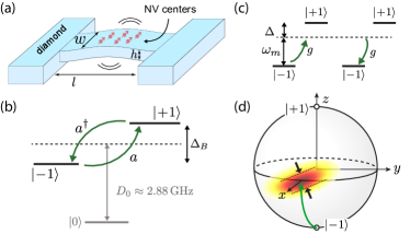
Figure 1: (a) All-diamond doubly clamped mechanical resonator with an ensemble of embedded NV centers. (b) Spin triplet states of the NV electronic ground state. Local perpendicular strain induced by beam bending mixes the $\left|\pm 1\right\rangle$ states. (c) A collection spins in the two-level subspace $\{\left|+1\right\rangle,\left|-1\right\rangle\}$ is off-resonantly coupled to a common mechanical mode giving rise to effective spin-spin interactions. (d) Squeezing of the spin uncertainty distribution of an NV ensemble.

Model.—The electronic ground state of the negatively charged NV center is a spin $S=1$ triplet with spin states labeled by $\left|m_{s}=0,\pm 1\right\rangle$ as shown in Fig. 1b. In the presence of external electric and magnetic fields $\vec{E}$ and $\vec{B}$, the Hamiltonian for a single NV is $(\hbar=1)$ Doherty2012

$$\begin{split}H_{\rm NV}=&(D_{0}+d_{\parallel}E_{z})S_{z}^{2}+\mu_{B}g_{s}\vec{S}\cdot\vec{B}\\ &-d_{\perp}\left[E_{x}(S_{x}S_{y}+S_{y}S_{x})+E_{y}(S_{x}^{2}-S_{y}^{2})\right],\end{split}$$ (1)

where $D_{0}/2\pi\simeq 2.88$ GHz is the zero field splitting, $g_{s}\simeq 2$, $\mu_{B}$ is the Bohr magneton, and $d_{\parallel}$ ($d_{\perp}$) is the ground state electric dipole moment in the direction parallel (perpendicular) to the NV axis Vanoort1990 ; Dolde2011 .

Motion of the diamond nanoresonator changes the local strain at the position of the NV center, which results in an effective, strain-induced electric field Doherty2012 . We are interested in the near-resonant coupling of a single resonant mode of the nanobeam to the $\left|\pm 1\right\rangle$ transition of the NV, with Zeeman splitting $\Delta_{B}=g_{s}\mu_{B}B_{z}/\hbar$, as shown in Fig. 1b,c. The perpendicular component of strain $E_{\perp}$ mixes the $\left|\pm 1\right\rangle$ states. For small beam displacements, the strain is linear in its position and we write $E_{\perp}=E_{0}(a+a^{\dagger})$, where $a$ is the destruction operator of the resonant mechanical mode of frequency $\omega_{m}$, and $E_{0}$ is the perpendicular strain resulting from the zero point motion of the beam. We note that the parallel component of strain shifts both states $\left|\pm 1\right\rangle$ relative to $\left|0\right\rangle$ Acosta2010 ; however, with near-resonant coupling $\Delta=\Delta_{B}-\omega_{m}\ll D_{0}$ and preparation in the $\left|\pm 1\right\rangle$ subspace, the state $\left|0\right\rangle$ remains unpopulated and parallel strain plays no role in what follows. Within this two-level subspace, the interaction of each NV is $H_{i}=g\left(\sigma^{+}_{i}a+a^{\dagger}\sigma^{-}_{i}\right)$, where $\sigma^{\pm}_{i}=\left|\pm 1\right\rangle_{i}\left\langle\mp 1\right|$ is the Pauli operator of the $i$th NV center and $g$ is the single phonon coupling strength. For many NV centers we introduce collective spin operators, $J_{z}=\frac{1}{2}\sum_{i}\left|1\right\rangle_{i}\left\langle 1\right|-\left|-1\right\rangle_{i}\left\langle-1\right|$ and $J_{\pm}=J_{x}\pm iJ_{y}=\sum_{i}\sigma^{\pm}_{i}$, which satisfy the usual angular momentum commutation relations. The total system Hamiltonian can then be written as

$$H=\omega_{m}a^{\dagger}a+\Delta_{B}J_{z}+g\left(a^{\dagger}J_{-}+aJ_{+}\right),$$ (2)

which describes a Tavis-Cummings type interaction between an ensemble of spins and a single mechanical mode. In Eq. (2) we have assumed uniform coupling of each spin to the mechanical mode for simplicity. In general the coupling may be nonuniform and we discuss this further below.

To estimate the coupling strength $g$, we calculate the strain for a given mechanical mode and use the experimentally obtained stress coupling of $0.03$ Hz Pa^-1 in the NV ground state Togan2011 ; si . We take a doubly clamped diamond beam (see Fig. 1a) with dimensions $L\gg w,h$ such that Euler-Bernoulli thin beam elasticity theory is valid LL . For NV centers located near the surface of the beam we obtain si

$$\frac{g}{2\pi}\approx 180\left(\frac{\hbar}{L^{3}w\sqrt{\rho E}}\right)^{1/2}{\rm GHz},$$ (3)

where $\rho$ is the mass density and $E$ is the Young’s modulus of diamond. For a beam of dimensions $(L,w,h)=(1,0.1,0.1)\,\mu$m we obtain a vibrational frequency $\omega_{m}/2\pi\sim 1$ GHz and coupling $g/2\pi\sim 1$ kHz. While this is smaller than the strain coupling $g_{e}/2\pi\approx 10$ MHz expected for electronic excited states of defect centers Habraken2012 ; Soykal2011 or quantum dots Wilson-Rae2004 , we benefit from the much longer spin coherence time $T_{2}$ in the ground state. An important figure of merit is the single spin cooperativity $\eta=\frac{g^{2}T_{2}}{\gamma\bar{n}_{\rm th}}$, where $\gamma=\omega_{m}/Q$ is the mechanical damping rate and $\bar{n}_{\rm th}=(e^{\hbar\omega_{m}/k_{B}T}-1)^{-1}$ is the equilibrium phonon occupation number at temperature $T$. Assuming $Q=10^{6}$, $T_{2}=10$ ms and $T=4$ K, we obtain a single spin cooperativity of $\eta\sim 0.8$. This can be further increased by reducing the dimensions of the nanobeam and operating at lower temperatures.

Spin squeezing.—In the dispersive regime, $g\ll\Delta=\Delta_{B}-\omega_{m}$, virtual excitations of the mechanical mode result in effective interactions between the otherwise decoupled spins. In this limit, $H$ can be approximately diagonalized by the transformation $e^{R}He^{-R}$ with $R=\frac{g}{\Delta}\left(a^{\dagger}J_{-}-aJ_{+}\right)$. To order $(g/\Delta)^{2}$ this yields an effective Hamiltonian,

$$H_{\rm eff}=\omega_{m}a^{\dagger}a+\left(\Delta_{B}+\lambda a^{\dagger}a\right)J_{z}+\frac{\lambda}{2}J_{+}J_{-},$$ (4)

where $\lambda=2g^{2}/\Delta$ is the phonon-mediated spin-spin coupling strength. Rewriting $J_{+}J_{-}={\bf{J}}^{2}-J_{z}^{2}+J_{z}$, and provided the total angular momentum $J$ is conserved, we obtain a term $\propto J_{z}^{2}$ corresponding to the one-axis twisting Hamiltonian Kitagawa1993 .

To generate a spin squeezed state, we initialize the ensemble in a coherent spin state (CSS) $\left|\psi_{0}\right\rangle$ along the $x$ axis of the collective Bloch sphere. The CSS satisfies $J_{x}\left|\psi_{0}\right\rangle=J\left|\psi_{0}\right\rangle$ and has equal transverse variances, $\left\langle J_{y}^{2}\right\rangle=\left\langle J_{z}^{2}\right\rangle=J/2$. This can be achieved using optical pumping and global rotations of the spins with microwave fields Taylor2008 . The squeezing term $\propto J_{z}^{2}$ describes a precession of the collective spin about the $z$ axis at a rate proportional to $J_{z}$, resulting in a shearing of the uncertainty distribution and a reduced spin variance in one direction as shown in Fig. 1d. This is quantified by the squeezing parameter Wineland1992 ; Ma2011 ,

$$\xi^{2}=\frac{2J\left\langle\Delta J_{\rm min}^{2}\right\rangle}{\left\langle J_{x}\right\rangle^{2}},$$ (5)

where $\left\langle\Delta J_{\rm min}^{2}\right\rangle=\frac{1}{2}\left(V_{+}-\sqrt{V_{-}^{2}+V_{yz}^{2}}\right)$ is the minimum spin uncertainty with $V_{\pm}=\left\langle J_{y}^{2}\pm J_{z}^{2}\right\rangle$ and $V_{yz}=\left\langle J_{y}J_{z}+J_{z}J_{y}\right\rangle/2$. The preparation of a spin squeezed state, characterized by $\xi^{2}<1$, has direct implications for NV ensemble magnetometry applications, since it would enable magnetic field sensing with a precision below the projection noise limit Wineland1992 .

We now consider spin squeezing in the presence of realistic decoherence. In addition to the coherent dynamics described by $H_{\rm eff}$, we account for mechanical dissipation and spin dephasing using a master equation si

$$\dot{\rho}= -i\left[-\frac{\lambda}{2}J_{z}^{2}+\left(\Delta_{B}+\lambda a^{\dagger}a\right)J_{z},\rho\right]+\frac{1}{2T_{2}}\sum_{i}\mathcal{D}[\sigma_{z}^{i}]\rho$$

$$+{\Gamma_{\gamma}}(\bar{n}_{\rm th}+1)\mathcal{D}[J_{-}]+{\Gamma_{\gamma}}\bar{n}_{\rm th}\mathcal{D}[J_{+}],$$ (6)

where $\mathcal{D}[c]\rho=c\rho c^{\dagger}-\frac{1}{2}\left(c^{\dagger}c\rho+\rho c^{\dagger}c\right)$ and the single spin dephasing $T_{2}^{-1}$ is assumed to be Markovian for simplicity (see below). Note that we absorbed a shift of $\lambda/2$ into $\Delta_{B}$, and ignored single spin relaxation as $T_{1}$ can be several minutes at low temperatures Jarmola2012 . The second line describes collective spin relaxation induced by mechanical dissipation, with $\Gamma_{\gamma}=\gamma g^{2}/\Delta^{2}$. Finally, the phonon number $n=a^{\dagger}a$ shifts the spin frequency, acting as an effective fluctuating magnetic field which leads to additional dephasing.

Let us for the moment ignore fluctuations of the phonon number $n$; we address these in detail below. Starting from the CSS $|\psi_{0}\rangle$, we plot the squeezing parameter in Fig. 2a for an ensemble of $N=100$ spins and several values of $\bar{n}_{\rm th}$, in the presence of dephasing $T_{2}^{-1}$ and collective relaxation $\Gamma_{\gamma}$. Here we calculated $\xi^{2}$ by solving Eq. (Phonon-induced spin-spin interactions in diamond nanostructures: application to spin squeezing) using an approximate numerical approach treating $\Gamma_{\gamma}$ and $T_{2}$ separately, and verified that the approximation agrees with exact results for small $N$ si . To estimate the minimum squeezing, we linearize the equations of motion for the averages and variances of the collective spin operators (see dashed lines in Fig. 2a). From these linearized equations, in the limits of interest, $J\gg 1$, $\bar{n}_{\rm th}\gg 1$ and to leading order in both sources of decoherence, we obtain approximately

$$\xi^{2}\simeq\frac{4\Gamma_{\gamma}\bar{n}_{\rm th}}{J\lambda^{2}t}+\frac{t}{T_{2}}.$$ (7)

Optimizing $t$ and the detuning $\Delta$, we obtain the optimal squeezing parameter,

$$\xi^{2}_{\rm opt}\simeq\frac{2}{\sqrt{J\eta}},$$ (8)

at time $t_{\rm opt}=T_{2}/\sqrt{J\eta}$, similar to results for atomic systems SchleierSmith2010 ; Leroux2010 ; Leroux2012 . Note that for non-Markovian dephasing, the scaling is even more favorable Marcos2010 . In Fig. 2b we plot the scaling of the squeezing parameter with $J$ for small but finite decoherence, and find agreement with Eq. (8). For comparison we also plot the unitary result in the absence of decoherence, scaling as $\xi^{2}_{\rm opt}\sim J^{-2/3}$ and limited by the Bloch sphere curvature Kitagawa1993 .

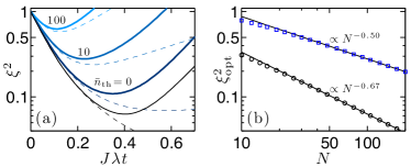
Figure 2: (a) Spin squeezing parameter versus scaled precession time with $N=100$ spins. Solid blue lines show the calculated squeezing parameter for $T_{2}=10$ ms and values of $\bar{n}_{\rm th}$ as shown. For each curve, we optimized the detuning $\Delta$ to obtain the optimal squeezing. Blue dashed lines are calculated from the linearized equations for the spin operator averages. Black solid (dashed) line shows exact (linearized) unitary squeezing. (b) Optimal squeezing versus number of spins. Lower (upper) red line shows power law fit for $\bar{n}_{\rm th}=1$ (10) and $T_{2}=1$ (0.01) s. The detuning $\Delta$ is optimized for each point. Other parameters in both plots are $\omega_{m}/2\pi=1$ GHz, $g/2\pi=1$ kHz, $Q=10^{6}$.

Phonon number fluctuations.—In Eq. (4) we see that the phonon number $n=a^{\dagger}a$ couples to $J_{z}$, leading to additional dephasing due to thermal number fluctuations. On the other hand, this same coupling can also lead to additional spin squeezing from cavity feedback, by driving the mechanical mode SchleierSmith2010 ; Leroux2010 ; Leroux2012 . In the following, we consider a twofold approach to mitigate thermal spin dephasing while preserving the optimal squeezing. First, we apply a sequence of global spin echo control pulses to suppress dephasing from low-frequency thermal fluctuations. This also extends the effective coherence time $T_{2}$ of single NV spins Taylor2008 . Second, we consider driving the mechanical mode, and identify conditions when this results in a net improvement of the squeezing.

To simultaneously account for thermal dephasing, driven feedback squeezing, and spin control pulse sequences, we write the interaction term in Eq. (4) in the so-called “toggling frame” Haeberlen1968 ,

$$H_{\rm int}(t)=\lambda J_{z}f(t)\delta n(t).$$ (9)

The function $f(t)$ periodically inverts the sign of the interaction as shown in the inset of Fig. 3a, describing the inversion of the collective spin $J_{z}\rightarrow-J_{z}$ with each $\pi$ pulse of the spin echo sequence. Phonon number fluctuations are described by $\delta n(t)=n(t)-\bar{n}$, where $\bar{n}$ is the mean phonon number and we have omitted an average frequency shift proportional to $\bar{n}$ in Eq. (9). The number fluctuation spectrum $S_{n}(\omega)=\int dte^{i\omega t}\left\langle\delta n(t)\delta n(0)\right\rangle$ is plotted in Fig. 3a for a driven oscillator coupled to a thermal bath si .

We calculate the required spin moments within the Gaussian approximation for phonon number fluctuations, and obtain si

$$\left\langle J_{+}(t)\right\rangle=e^{-\chi}\left\langle e^{-i\mu(J_{z}-1/2)}J_{+}(0)\right\rangle,$$ (10)

and similar results for $\left\langle J_{+}^{2}(t)\right\rangle$ and $\left\langle J_{+}(t)J_{z}(t)\right\rangle$. In Eq. (10) the dephasing parameter $\chi$ and effective squeezing via $\mu$ are given by

$$\chi =\lambda^{2}\int\frac{d\omega}{2\pi}\frac{F(\omega\tau)}{\omega^{2}}\bar{S}_{n}(\omega),$$ (11)

$$\mu =\lambda^{2}\int\frac{d\omega}{2\pi}\frac{K(\omega\tau)}{\omega^{2}}A_{n}(\omega),$$ (12)

where $\bar{S}_{n}(\omega)=\left(S_{n}(\omega)+S_{n}(-\omega)\right)/2$ and $A_{n}(\omega)=\left(S_{n}(\omega)-S_{n}(-\omega)\right)/2$. The filter function $F(\omega\tau)=\frac{\omega^{2}}{2}\left|\int dte^{i\omega t}f(t)\right|^{2}$ describes the effect of the spin echo pulse sequence with time $\tau$ between $\pi$ pulses Martinis2003 ; Uhrig2007 ; Cywinski2008 . The function $K(\omega\tau)$ plays the analogous role for the effective squeezing described by $\mu$, and is related to $F$ by a Kramers-Kronig relation si . We plot $K$ and $F$ for a sequence of $M=4$ pulses in Fig. 3a.

Discussion.—We now consider the impact of thermal fluctuations on the achievable squeezing. The noise spectrum $S_{n}(\omega)=2\gamma\bar{n}_{\rm th}(\bar{n}_{\rm th}+1)/(\omega^{2}+\gamma^{2})$ is symmetric around $\omega=0$. Without spin echo control pulses, this low frequency noise results in nonexponential decay of the spin coherence, $\chi_{0}(t)=\frac{1}{2}\lambda^{2}\bar{n}_{\rm th}^{2}t^{2}$ (with $\bar{n}_{\rm th}\gg 1$), familiar from single qubit decoherence Taylor2008 ; deSousa2009 . The inhomogeneous thermal dephasing time is $T_{2}^{*}\simeq\sqrt{2}/\lambda\bar{n}_{\rm th}$, severely limiting the possibility of spin squeezing. In particular, at time $t=t_{\rm opt}$ we find that squeezing is prohibited when $\bar{n}_{\rm th}>\sqrt{J}$ si . However, one can overcome this low frequency thermal noise using spin echo. By applying a sequence of $M$ equally spaced global $\pi$-pulses to the spins during precession of total time $t$, we obtain $\chi_{\rm th}\sim\lambda^{2}\gamma\bar{n}_{\rm th}^{2}t^{3}/M^{2}$, suggesting that thermal dephasing can be made negligible relative to both $\Gamma_{\gamma}$ and $T_{2}^{-1}$. For a sufficiently large number of pulses, $M\gg\bar{n}_{\rm th}\sqrt{\gamma T_{2}}$, we recover the optimal squeezing in Eqs. (7) and (8).

Adding a mechanical drive can further enhance squeezing via feedback; however, it also increases phonon number fluctuations, contributing to additional dephasing. We consider a detuned external drive of frequency $\omega_{\rm dr}=\omega_{m}+\delta$, leading to two additional peaks in $S_{n}(\omega)$ at $\omega=\pm\delta$, as shown in Fig. 3a. The area under the left [right] peak scales as $\bar{n}_{\rm dr}\bar{n}_{\rm th}$ [$\bar{n}_{\rm dr}(\bar{n}_{\rm th}+1)$], where $\bar{n}_{\rm dr}$ is the mean phonon number due to the drive at zero temperature. The symmetric and antisymmetric parts of this noise contribute to dephasing and squeezing as described by Eqs. (11) and (12). Choosing the interval $t/M=2\pi/\delta$ between $\pi$ pulses, we obtain additional dephasing $\chi_{\rm dr}\simeq\left(\frac{\lambda}{\delta}\right)^{2}\bar{n}_{\rm dr}\bar{n}_{\rm th}\gamma t$ and effective squeezing with $\mu\simeq\frac{\lambda^{2}}{\delta}\bar{n}_{\rm dr}t$. In the limit $\bar{n}_{\rm dr}\gg\bar{n}_{\rm th}$, the effects of the drive dominate over $\chi_{\rm th}$ and $\Gamma_{\gamma}$ and we recover the ideal scaling given in Eq. (8), even with a small number of echo pulses. This is shown in Fig. 3b,c where we see that the optimal squeezing improves with increasing $\bar{n}_{\rm dr}$ for a fixed number of pulses $M=4$.

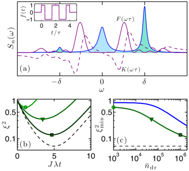
Figure 3: (a) Number fluctuation spectrum of thermal driven oscillator. Center (blue) peak is purely thermal while side (green) peaks are due to detuned drive. Solid (dashed) purple line shows filter function $F$ ($K$) for $M=4$ pulses. Inset: corresponding function $f(t)$ for $M=4$. (b) Solid green curves show squeezing parameter versus precession time for $\bar{n}_{\rm th}=10$ and $\bar{n}_{\rm dr}=10^{3},5\times 10^{4},10^{6}$ (top to bottom). Dashed black line shows unitary squeezing. (c) Minimum squeezing versus drive strength for $\bar{n}_{\rm th}=50,10$ (top to bottom). Symbols mark corresponding points with (b). Dashed black line shows unitary squeezing. Parameters in (b) and (c) are $M=4$, $g/2\pi=1$ kHz, $T_{2}=10$ ms, $N=100$, $\omega_{m}/2\pi=1$ GHz, $Q=10^{6}$.

Finally, we discuss our assumption of uniform coupling strength $g$ in Eq. (2). This is an important practical issue, as we expect the coupling to individual spins to be inhomogeneous in experiment due to the spatial variation of strain in the beam. Nonetheless, even with nonuniform coupling, we still obtain squeezing of a collective spin with a reduced effective total spin $J_{\rm eff}<J$, provided $J\gg 1$. First, we note that inhomogeneous magnetic fields resulting in nonuniform detuning are compensated by spin echo. Second, for a distribution of coupling strengths $g_{i}$, the effective length of the collective spin is $\sum_{i}g_{i}/\sqrt{\sum_{i}g_{i}^{2}}$ for the direct squeezing term, and $\sum_{i}g_{i}^{2}/\sqrt{\sum_{i}g_{i}^{4}}$ for feedback squeezing with a mechanical drive. Similar conclusions were reached in atomic and nuclear systems SchleierSmith2010 ; Leroux2010 ; Leroux2012 ; Rudner2011 . In the case of direct squeezing, it is important that the sign of the $g_{i}$’s is the same to avoid cancellation; this is automatically achieved by using NV centers implanted on the top of the beam. For beam dimensions $(1,0.1,0.1)\,\mu$m analyzed above, we estimate that $N\sim 200$ NV centers can be embedded without being perturbed by direct magnetic dipole-dipole interactions. A reduction of the effective spin length by factor $\sim 2$ still leaves $N_{\rm eff}\sim 100$, sufficient to observe spin squeezing.

Conclusions.—We have shown that direct spin-phonon coupling in diamond can be used to prepare spin squeezed states of an NV ensemble embedded in a nanoresonator, even in the presence of dephasing and mechanical dissipation. With further reductions in temperature, beam dimensions, and spin decoherence rates, the regime of large single spin cooperativity $\eta\gg 1$ could be achieved. This would allow for coherent phonon-mediated interactions and quantum gates between two spins embedded in the same resonator via $H_{\rm int}=\lambda\left(\sigma^{+}_{1}\sigma^{-}_{2}+{\rm h.c.}\right)$, and coupling over larger distances by phononic channels Habraken2012 .

Acknowledgments.—The authors gratefully acknowledge discussions with Shimon Kolkowitz and Quirin Unterreithmeier. This work was supported by NSF, CUA, DARPA, NSERC, HQOC, DOE, the Packard Foundation, the EU project AQUTE and the Austrian Science Fund (FWF) through SFB FOQUS and the START grant Y 591-N16.

I Supplemental information

I.1 Coupling strength

We assume that the NV axis is aligned with both the magnetic field and with the direction of beam deflection, so that the longitudinal strain due to deflection is entirely perpendicular to the NV axis. From experiment Togan2010supp , the splitting of the $\left|\pm 1\right\rangle$ states with stress is $\sim 0.03$ Hz/Pa. We convert this into the deformation potential coupling frequency, $\Xi/2\pi\hbar=36$ GHz, using the Young’s modulus of diamond, $E=1200$ GPa. Next we calculate the strain at the NV center using elasticity theory. The equation for the bending mode of a thin beam is

$$\rho A\partial_{t}^{2}\phi(z,t)=-EI\partial_{z}^{4}\phi(z,t)$$ (13)

where $\phi$ is the transverse displacement in the $x$ direction and $z$ is along the beam. Here $\rho$ is the mass density, $A$ is the cross sectional area, and $I=wt^{3}/12$ is the moment of inertia. The solutions are of the form $\phi(z,t)=u(z)e^{-i\omega t}$ where

$$\begin{split}u(z)=\frac{1}{\sqrt{N}}\Big{[}&\cos kz-\cosh kz\\ &-\frac{(\cos kL-\cosh kL)}{(\sin kL-\sinh kL)}(\sin kz-\sinh kz)\Big{]},\end{split}$$ (14)

which satisfies the boundary conditions $u(0)=u^{\prime}(0)=u(L)=u^{\prime}(L)=0$ for a doubly clamped beam. The allowed wavenumbers $k_{n}$ are given by the solutions of $\cos kL\cosh kL=1$, and the corresponding eigenfrequencies are

$$\omega_{n}=k_{n}^{2}\sqrt{\frac{EI}{\rho A}}.$$ (15)

We normalize the modefunction of the fundamental mode $u_{0}(z)$ by setting the free energy stored in the beam to the zero point energy,

$$W=\frac{1}{2}EI\int_{0}^{L}dz\left(\frac{\partial^{2}u_{0}}{\partial z^{2}}\right)^{2}=\frac{\hbar\omega_{0}}{2}.$$ (16)

Integrating by parts we obtain the normalization condition,

$$\int_{0}^{L}dzu_{0}^{2}=\frac{\hbar}{\rho A\omega_{0}}.$$ (17)

If the NV center lies at the midpoint along the beam, $z=L/2$, and at a distance $r_{0}$ from the neutral axis of the beam, the strain due to the zero point motion of the fundamental mode is

$$\epsilon_{0}=-r_{0}\partial_{z}^{2}u_{0}(L/2)\sim r_{0}\sqrt{\frac{\hbar}{\rho A\omega_{0}}}\frac{27}{L^{5/2}}\sim 5\frac{2r_{0}}{t}\sqrt{\frac{\hbar}{L^{3}w\sqrt{E\rho}}},$$ (18)

where we Eq. (15) and $k_{0}\sim 4.73/L$ for the fundamental mode. The coupling strength is given by the deformation potential and the strain due to zero point motion,

$$\frac{g}{2\pi}=\frac{\Xi}{2\pi\hbar}\epsilon_{0}\sim 180\ {\rm GHz}\cdot\frac{2r_{0}}{t}\sqrt{\frac{\hbar}{L^{3}w\sqrt{E\rho}}}.$$ (19)

For an NV near the surface of the beam, $r_{0}\sim t/2$ and we obtain Eq. (4) of the main text.

I.2 Effective squeezing Hamiltonian from spin-phonon coupling

In this section we provide additional details on deriving $H_{\rm eff}$ in Eq. (4) from the original $H_{\rm NV}$ in Eq. (1). Assuming that the magnetic field is aligned along the NV axis, $\vec{B}=B\hat{z}$, and defining $E_{\pm}=E_{x}\pm iE_{y}$ and $S_{\pm}=S_{x}\pm iS_{y}$, we can rewrite $H_{\rm NV}$ as ($\hbar=1$)

$$H_{\rm NV}=(D_{0}+d_{\parallel}E_{z})S_{z}^{2}+g_{s}\mu_{B}BS_{z}-\frac{{d_{\perp}}}{2}\left(E_{+}S_{+}^{2}+E_{-}S_{-}^{2}\right),$$ (20)

where $\vec{E}$ is the effective electric field due to strain. We quantize the perpendicular strain field, $E_{+}=E_{0}a$ and $E_{-}=E_{0}a^{\dagger}$, where $E_{0}$ is the strain due to the zero point motion of the resonant mode. Next we focus on the two-level subspace $\{\left|1\right\rangle,\left|-1\right\rangle\}$ only, and assume that transitions to state $\left|0\right\rangle$ are not allowed due to the large zero field splitting $D_{0}$. For the $i$th spin we write Pauli operators $\sigma^{\pm}_{i}=\left|\pm 1\right\rangle_{i}\left\langle\mp 1\right|$ and $\sigma^{z}_{i}=\left|1\right\rangle_{i}\left\langle 1\right|-\left|-1\right\rangle_{i}\left\langle-1\right|$, and within this two-level subspace the interaction for a single NV is

$$H_{i}=\frac{\Delta_{B}}{2}\sigma^{z}_{i}+g\left(\sigma^{+}_{i}a+a^{\dagger}\sigma^{-}_{i}\right)+\omega_{m}a^{\dagger}a,$$ (21)

where $g=-d_{\perp}E_{0}$, $\Delta_{B}=2g_{s}\mu_{B}B$ is the energy between $\left|\pm 1\right\rangle$, and we included the mechanical oscillator of frequency $\omega_{m}$. Summing Eq. (21) for many NVs coupled to the same mode with uniform coupling strength we obtain

$$H=\Delta_{B}J_{z}+g\left(a^{\dagger}J_{-}+aJ_{+}\right)+\omega_{m}a^{\dagger}a,$$ (22)

which is Eq. (2) of the main text. To obtain Eq. (4), we first rewrite $H$ in the rotating frame at the mechanical frequency $\omega_{m}$,

$$H=\Delta J_{z}+g\left(a^{\dagger}J_{-}+aJ_{+}\right),$$ (23)

where $\Delta=\Delta_{B}-\omega_{m}$. Next we apply the transformation $e^{R}He^{-R}$, with $R=\frac{g}{\Delta}\left(a^{\dagger}J_{-}-aJ_{+}\right)$, and to order $(g/\Delta)^{2}$ we obtain

$$H_{\rm eff}\simeq\Delta J_{z}+\frac{g^{2}}{\Delta}\left(J_{+}J_{-}+2a^{\dagger}aJ_{z}\right).$$ (24)

Transforming back to the nonrotating frame yields Eq. (4) of the main text.

I.3 Individual spin dephasing and phonon-induced relaxation

I.3.1 Individual spin dephasing from intrinsic $T_{2}$

Each NV spin experiences intrinsic decoherence in the absence of the mechanical mode. Individual relaxation ($T_{1}$) processes are due to lattice phonons; at low temperature $T_{1}$ can be $\sim 100$ s and we ignore it Jarmola2012supp . However, we include intrinsic single spin dephasing, which arises from magnetic noise of ¹³C nuclear spins in the diamond lattice. In practice, single spin dephasing may be nonexponential Taylor2008supp ; deSousa2009supp , but for simplicity we approximate the effect of single spin dephasing by an effective Markovian master equation with dephasing rate $T_{2}^{-1}$,

$$\dot{\rho}=\frac{1}{2T_{2}}\sum_{i}\left[\sigma^{z}_{i}\rho\sigma^{z}_{i}-\rho\right].$$ (25)

I.3.2 Collective phonon-induced spin relaxation

The transformation $R$ used to obtain the effective squeezing Hamiltonian $H_{\rm eff}$ also introduces a relaxation channel for the collective spin by admixing phonon and spin degrees of freedom. Mechanical dissipation is described by the master equation for the system density matrix $\rho$,

$$\begin{split}\dot{\rho}=&\gamma(\bar{n}_{\rm th}+1)\left[a\rho a^{\dagger}-\tfrac{1}{2}\left(a^{\dagger}a\rho+\rho a^{\dagger}a\right)\right]\\ &+\gamma\bar{n}_{\rm th}\left[a^{\dagger}\rho a-\tfrac{1}{2}\left(aa^{\dagger}\rho+\rho aa^{\dagger}\right)\right].\end{split}$$ (26)

Transforming $a$ and $a^{\dagger}$ using the transformation $R$ in the main text, we obtain effective spin relaxation terms in the master equation,

$$\begin{split}\dot{\rho}=&\Gamma_{\gamma}(\bar{n}_{\rm th}+1)\left[J_{-}\rho J_{+}-\tfrac{1}{2}\left(J_{+}J_{-}\rho+\rho J_{+}J_{-}\right)\right]\\ &+\Gamma_{\gamma}\bar{n}_{\rm th}\left[J_{+}\rho J_{-}-\tfrac{1}{2}\left(J_{-}J_{+}\rho+\rho J_{-}J_{+}\right)\right]\end{split}$$ (27)

where $\Gamma_{\gamma}=\left(\frac{g}{\Delta}\right)^{2}\gamma$. From Eqs. (25) and (27) we calculate the equations for spin averages and variances accounting for individual dephasing and collective relaxation using $\partial_{t}\left\langle A\right\rangle=\text{tr}{\left\{A\dot{\rho}\right\}}$.

I.3.3 Squeezing estimate from linearized equations for spin averages and variances

Here we sketch the derivation of the estimated optimal squeezing given in Eq. (8) in the main text. In order to treat the squeezing Hamiltonian, collective relaxation and spin dephasing on equal footing, we linearize the equations for the spin averages and variances. This corresponds to expanding in the small error from decoherence at short times and ignoring the curvature of the Bloch sphere for sufficiently short times, when the spin uncertainty distribution remains on a locally flat region of the Bloch sphere. To linearize the equations we assume that all (connected) correlations of order higher than two vanish. The linearized equations are valid for short times, so we also make use of the initial conditions in the spin coherent state at $t=0$, which are $\left\langle J_{y}\right\rangle=\left\langle J_{z}\right\rangle=\left\langle C_{yz}\right\rangle=0$ and $\left\langle J_{y}^{2}\right\rangle=\left\langle J_{z}^{2}\right\rangle=J/2$. Here we define the covariance operator $C_{yz}=(J_{y}J_{z}+J_{z}J_{y})/2$, while in the main text we refer only to its average, $V_{yz}=\left\langle C_{yz}\right\rangle$. Within these approximations, and using Eqs. (25) and(27), the linearized equations for the spin averages required to calculate the squeezing parameter $\xi^{2}$ are

$$\partial_{t}\left\langle J_{x}\right\rangle =-\Gamma_{2}\left\langle J_{x}\right\rangle$$ (28)

$$\partial_{t}\left\langle J_{y}\right\rangle =\lambda J\left\langle J_{z}\right\rangle-\Gamma_{2}\left\langle J_{y}\right\rangle-\Gamma_{\gamma}(\bar{n}_{\rm th}+\tfrac{1}{2})\left\langle J_{y}\right\rangle+\Gamma_{\gamma}\left\langle C_{yz}\right\rangle$$ (29)

$$\partial_{t}\left\langle J_{z}\right\rangle =-2\Gamma_{\gamma}(\bar{n}_{\rm th}+\tfrac{1}{2})\left\langle J_{z}\right\rangle-\Gamma_{\gamma}\left[J(J+1)-\left\langle J_{z}^{2}\right\rangle\right]$$ (30)

$$\partial_{t}\left\langle J_{y}^{2}\right\rangle =2J\lambda\left\langle C_{yz}\right\rangle-2\Gamma_{2}\left(\left\langle J_{y}^{2}\right\rangle-\frac{J}{2}\right)-2\Gamma_{\gamma}(\bar{n}_{\rm th}+\tfrac{1}{2})\left\langle J_{y}^{2}-J_{z}^{2}\right\rangle+\Gamma_{\gamma}J\left\langle J_{z}\right\rangle+\frac{\Gamma_{\gamma}}{2}\left\langle J_{z}\right\rangle$$ (31)

$$\partial_{t}\left\langle J_{z}^{2}\right\rangle =-2\Gamma_{\gamma}(\bar{n}_{\rm th}+\tfrac{1}{2})\left[3\left\langle J_{z}^{2}\right\rangle-J(J+1)\right]+\Gamma_{\gamma}\left\langle J_{z}\right\rangle\left[1-2J(J+\tfrac{1}{2})\right]$$ (32)

$$\partial_{t}\left\langle C_{yz}\right\rangle =\lambda J\left\langle J_{z}^{2}\right\rangle-\Gamma_{2}\left\langle C_{yz}\right\rangle-5\Gamma_{\gamma}(\bar{n}_{\rm th}+\tfrac{1}{2})\left\langle C_{yz}\right\rangle-\Gamma_{\gamma}\left(J^{2}-\tfrac{1}{4}\right)\left\langle J_{y}\right\rangle$$ (33)

This linear set of equations can be directly solved. The full analytic solutions are lengthy so we simply plot the numerical solution for the squeezing parameter (blue dash-dotted in Fig. 4), which agrees with exact numerics at short times.

We use these linearized equations to estimate the scaling of the optimal squeezing parameter (see Eqs. (7) and (8) in the main text). First, we solve Eqs. (28-33) to second order in $t$. Second, we calculate $\xi^{2}$ (see Eq. (5) in the main text) from the resulting spin averages, and simplify the result in the limit of interest, $J\gg 1,\bar{n}_{\rm th}\gg 1$, and assuming $J\lambda t\gg 1$ as required for significant squeezing. Third, we assume that all sources of decoherence are small, and expand in the errors $\Gamma_{\gamma}\bar{n}_{\rm th}t\ll 1$ and $\Gamma_{2}t\ll 1$. Within these approximations we obtain

$$\xi^{2}\simeq\frac{1+4J\Gamma_{\gamma}\bar{n}_{\rm th}t}{\left(J\lambda t\right)^{2}}+\left(5\Gamma_{\gamma}\bar{n}_{\rm th}+T_{2}^{-1}\right)t,$$ (34)

where the first term $1/(J\lambda t)^{2}$ is the result from linearized unitary squeezing, and the remaining terms are the lowest order corrections in both sources of decoherence. We further approximate $T_{2}^{-1}\gg\Gamma_{\gamma}\bar{n}_{\rm th}$, valid for sufficiently large detuning $\Delta$, and $J\Gamma_{\gamma}\bar{n}_{\rm th}t\gg 1$, valid self-consistently at the optimal squeezing time and in the relevant limit $J\gg\eta$. Within these approximations we obtain Eq. (7) in the main text. Finally, we optimize $\xi^{2}$ with respect to $t$, obtaining Eq. (8) and $t_{\rm opt}$ given in the main text.

I.3.4 Combining individual dephasing and collective relaxation: numerics

As discussed in the main text, in the absence of a mechanical drive we can neglect phonon number fluctuations for a sufficiently large number of $\pi$ pulses $M$. In this case the remaining sources of decoherence are intrinsic single spin dephasing and collective relaxation induced by mechanical dissipation. These sources of decoherence are simple to treat separately but difficult to treat simultaneously for a large number of spins. To calculate the solid blue curves in Fig. 2 of the main text, we treat the combination of both sources of decoherence as approximately independent, valid provided both are small enough to still allow spin squeezing. To calculate the spin averages needed for the squeezing parameter, we first account for collective relaxation using the Dicke state basis in which total $J$ is conserved. We then account for individual dephasing by multiplying the resulting averages by dephasing factors such as $\left\langle J_{x}(t)\right\rangle=e^{-t/T_{2}}\left\langle J_{x}(t)\right\rangle_{\rm D}$ where $\left\langle J_{x}(t)\right\rangle_{\rm D}$ is the result of the Dicke state calculation. Each step would be numerically exact in the absence of the other source of decoherence; thus we expect that this procedure provides a good approximation if all errors are small. To verify the accuracy of the approach, we compare the result with exact numerics calculated by numerically integrating the full master equation for small $N$ in Fig. 4.

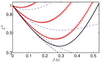
Figure 4: Spin squeezing parameter versus scaled precession time with $N=8$ spins. Solid red lines show squeezing calculated using the approximation discussed in the text, treating single spin dephasing and collective relaxation independently, with $\bar{n}_{\rm th}=0,10,100$ (bottom to top). Red dots show the exact numerics. The detuning $\Delta$ is optimized for each value of $\bar{n}_{\rm th}$. Blue dash-dotted lines show squeezing from linearized equations. Solid black line shows unitary squeezing, dashed black line shows unitary squeezing from linearized equations. Parameters are $\omega_{m}/2\pi=1$ GHz, $g/2\pi=1$ kHz, $Q=10^{6}$, $T_{2}=100$ ms.

I.4 Phonon number fluctutions

In this section we consider fluctuations of the phonon number, $n=a^{\dagger}a$. We start by rewriting the effective Hamiltonian [see Eq. (4) in main text] for the collective spin coupled to a driven oscillator in the frame rotating at the mechanical drive frequency,

$$H_{\rm eff}=\Delta J_{z}+\lambda J_{z}a^{\dagger}a+\frac{\lambda}{2}J_{z}^{2}-\delta a^{\dagger}a+\Omega(a+a^{\dagger})$$ (35)

where $\Delta=\Delta_{B}-\omega_{d}$ is the detuning of the magnetic transition frequency from the drive, and $\delta=\omega_{d}-\omega_{m}$ is the drive detuning from the mechanical frequency. The amplitude of the drive is $\Omega$ and we have made the rotating wave approximation. Our aim is to find the effect of the oscillator on the spin to second order in $\lambda$ (within the Gaussian approximation). For this we require the number fluctuation spectrum of a damped, driven, thermal oscillator in the absence of coupling to the spin.

I.4.1 Number fluctuations of a driven thermal mode

To calculate the effective dephasing from number fluctuations, we first need the power spectral density of phonon number fluctuations,

$$S_{n}(\omega)=\int dte^{i\omega t}\left\langle\delta n(t)\delta n(0)\right\rangle,$$ (36)

where $n=a^{\dagger}a$, $\delta n=n-\left\langle n\right\rangle$ and the average is taken with respect to the oscillator in thermal equilibrium with its environment. In the absence of coupling, $\lambda=0$, the Langevin equation for the driven thermal mode in the frame of the classical drive frequency and within the rotating wave approximation is

$$\dot{a}(t)=\left(i\delta-\frac{\gamma}{2}\right)a(t)+\Omega+\sqrt{\gamma}\xi(t)$$ (37)

The solution is $a(t)=\alpha+d(t)$, where $\alpha=\frac{\Omega}{-i\delta+\gamma/2}$ is the coherent amplitude due to the drive, and

$$d(t)=\sqrt{\gamma}\int_{-\infty}^{t}dt^{\prime}e^{i\delta-\gamma/2)(t-t^{\prime})}\xi(t^{\prime})$$ (38)

describes thermal and quantum fluctuations. The mean phonon number is the sum of driven and thermal parts, $\bar{n}=\bar{n}_{\rm dr}+\bar{n}_{\rm th}$, where

$$\bar{n}_{\rm dr}=\left|\alpha^{2}\right|=\frac{\Omega^{2}}{\delta^{2}+\gamma^{2}/4}\\$$ (39)

and the thermal occupation is $\bar{n}_{\rm th}=\left\langle d^{\dagger}d\right\rangle=1/(e^{\omega_{m}/T}-1)$. Using Eq. (38) we find the two-time correlations,

$$\left\langle d^{\dagger}(t)d(0)\right\rangle =\bar{n}_{\rm th}e^{-i\delta t}e^{-\gamma\left|t\right|/2},$$ (40)

$$\left\langle d(t)d^{\dagger}(0)\right\rangle =(\bar{n}_{\rm th}+1)e^{i\delta t}e^{-\gamma\left|t\right|/2},$$ (41)

and from these we can calculate the full spectrum of driven thermal number fluctuations. The correlation using Wick’s theorem and $a(t)=\alpha+d(t)$ is

$$\left\langle\left\langle\delta n(t)\delta n(0)\right\rangle\right\rangle= \left\langle n(t)n(0)\right\rangle-\bar{n}^{2}$$

$$= \bar{n}_{\rm dr}\left[\left\langle d^{\dagger}(t)d(0)\right\rangle+\left\langle d(t)d^{\dagger}(0)\right\rangle\right]$$ (42)

$$+\left\langle d^{\dagger}(t)d(0)\right\rangle\left\langle d(t)d^{\dagger}(0)\right\rangle.$$ (43)

Using Eq. (38) and taking the Fourier transform, we find that the number fluctuation spectrum for a driven thermal oscillator is given by

$$\begin{split}S_{n}(\omega)=&\gamma\bar{n}_{\rm dr}\left[\frac{\bar{n}_{\rm th}}{(\omega-\delta)^{2}+\gamma^{2}/4}+\frac{\bar{n}_{\rm th}+1}{(\omega+\delta)^{2}+\gamma^{2}/4}\right]\\ &+\frac{2\gamma\bar{n}_{\rm th}(\bar{n}_{\rm th}+1)}{\omega^{2}+\gamma^{2}}.\end{split}$$ (44)

I.4.2 Effects of number fluctuations on the spin in the Gaussian approximation

From the spectrum of number fluctuations we can calculate the effect of number fluctutions on the spin dephasing and squeezing. We write the full Hamiltonian as $H_{\rm eff}=H_{0}+H_{\rm osc}+H_{\rm int}$, where $H_{\rm osc}$ describes the driven damped oscillator, and

$$H_{0}=\Delta J_{z}+\frac{\lambda}{2}J_{z}^{2}$$ (45)

describes the spin including the constant effective squeezing term. The coupling in the interaction picture and in the toggling frame is

$$H_{\rm int}(t)=\lambda f(t)\delta n(t)J_{z},$$ (46)

where $J_{z}$ is time-independent as it commutes with the full Hamiltonian. We have included the function $f(t)$ to describe spin echo, which effectively inverts the sign of the interaction with each $\pi$ pulse.

The equation of motion for the operator $J_{+}$ in the interaction picture is

$$\dot{J}_{+}(t)=i\lambda f(t)\big{[}J_{z}\delta n(t),J_{+}(t)\big{]}.$$ (47)

We integrate this formally, insert the solution, and take the average with respect to the oscillator to get

$$\dot{J}_{+}(t)=-\lambda^{2}f(t)\int_{0}^{t}f(t^{\prime})\left\langle\big{[}J_{z}\delta n(t)\left[J_{z}\delta n(t^{\prime}),J_{+}(t^{\prime})\right]\big{]}\right\rangle_{\rm osc}$$ (48)

where $\left\langle\cdot\right\rangle_{\rm osc}$ denotes averaging over the oscillator degrees of freedom. Note that we neglected additional noise terms; these play no role as we will only be interested in taking the average at the end. Next, we neglect the time dependence of $J_{+}(t^{\prime})$ under the integral, as it is higher order in $\lambda$, $J_{+}(t)=e^{iH_{0}t}J_{+}e^{-iH_{0}t}=e^{i\lambda(J_{z}-1/2)t}J_{+}$. Expanding the commutators we obtain

$$\dot{J}_{+} =-\lambda^{2}f(t)\int_{0}^{t}f(t^{\prime})\left[J_{z}J_{+}\left\langle\delta n(t)\delta n(t^{\prime})\right\rangle-J_{+}J_{z}\left\langle\delta n(t^{\prime})\delta n(t)\right\rangle\right]$$

$$=-\lambda^{2}f(t)\int_{0}^{t}f(t^{\prime})\int\frac{d\omega}{2\pi}e^{-i\omega(t-t^{\prime})}\left[J_{z}J_{+}S_{n}(\omega)-J_{+}J_{z}S_{n}(-\omega)\right],$$ (49)

using Eq. (36). Defining the symmetric and antisymmetric parts of the number fluctuation spectrum,

$$\bar{S}_{n}(\omega)={\frac{1}{2}}\left[S_{n}(\omega)+S_{n}(-\omega)\right],\quad A_{n}(\omega)=S_{n}(\omega)-S_{n}(-\omega),$$ (50)

we can rewrite Eq. (49) as

$$\dot{J}_{+}=-\lambda^{2}f(t)\int_{0}^{t}f(t^{\prime})\int\frac{d\omega}{2\pi}e^{-i\omega(t-t^{\prime})}\times\left[\bar{S}_{n}(\omega)+A_{n}(\omega)\left(J_{z}-\frac{1}{2}\right)\right]J_{+}.$$ (51)

Solving Eq. (51) and finally taking the average with respect to spin degrees of freedom, we obtain

$$\left\langle J_{+}(t)\right\rangle=e^{-\chi}\left\langle e^{i\mu(J_{z}-\frac{1}{2})}J_{+}(0)\right\rangle$$ (52)

where $\left\langle\cdot\right\rangle$ is the average over all degrees of freedom, and

$$\chi =\lambda^{2}\int\frac{d\omega}{2\pi}\bar{S}_{n}(\omega)\int dt_{1}\int dt_{2}e^{-i\omega(t_{1}-t_{2})}\theta(t_{1}-t_{2})f(t_{1})f(t_{2}),$$ (53)

$$\mu =i\lambda^{2}\int\frac{d\omega}{2\pi}A_{n}(\omega)\int dt_{1}\int dt_{2}e^{-i\omega(t_{1}-t_{2})}\theta(t_{1}-t_{2})f(t_{1})f(t_{2}).$$ (54)

Here all integration limits are from $-\infty$ to $\infty$, and the time integration limits are accounted for in $f(t^{\prime})\propto\theta(t^{\prime})\theta(t-t^{\prime})$ and the step function $\theta(t_{1}-t_{2})$. Similarly, we obtain the other averages needed to calculate the squeezing,

$$\left\langle J_{+}^{2}(t)\right\rangle =e^{-4\chi}\left\langle e^{2i\mu(J_{z}-1)}J_{+}^{2}(0)\right\rangle,$$ (55)

$$\left\langle J_{+}(t)J_{z}(t)\right\rangle =e^{-\chi}\left\langle e^{i\mu\left(J_{z}-\frac{1}{2}\right)}J_{+}(0)J_{z}(0)\right\rangle.$$ (56)

By comparing with the spin evolution under unitary one-axis twisting, we see that $\mu$ describes spin squeezing with an effective squeezing coefficient $\lambda_{\rm eff}=\mu/t$. The parameter $\chi$ describes collective dephasing.

To evaluate $\chi$ and $\mu$ for a given pulse sequence, we next define $f(\omega)=\int dte^{i\omega t}f(t)$ to rewrite the double time integral as

$$I_{t}= \int dt_{1}\int dt_{2}e^{-i\omega(t_{1}-t_{2})}\theta(t_{1}-t_{2})f(t_{1})f(t_{2})$$ (57)

$$=\int\frac{d\omega_{1}}{2\pi}\left|f(\omega_{1})\right|^{2}\left[\pi\delta(\omega+\omega_{1})-\frac{i}{\omega+\omega_{1}}\right].$$ (58)

We define the filter function for pulse sequence with time $\tau$ between $\pi$ pulses,

$$F(\omega\tau)=\frac{\omega^{2}}{2}\left|f(\omega)\right|^{2}.$$ (59)

The dephasing term is

$$\chi =2\lambda^{2}\int\frac{d\omega}{2\pi}\bar{S}_{n}(\omega)\int\frac{d\omega_{1}}{2\pi}\frac{F(\omega_{1}\tau)}{\omega_{1}^{2}}\left[\pi\delta(\omega+\omega_{1})-\frac{i}{\omega+\omega_{1}}\right]$$ (60)

Since $F(\omega\tau)$ and $\bar{S}_{n}(\omega)$ are both even in $\omega$, the imaginary part of the integrand is odd and integrates to zero. As a result $\chi$ is real and we obtain

$$\chi=\lambda^{2}\int\frac{d\omega}{2\pi}\frac{F(\omega\tau)}{\omega^{2}}\bar{S}_{n}(\omega).$$ (61)

The coherent term is

$$\mu =i\lambda^{2}\int\frac{d\omega}{2\pi}A_{n}(\omega)\int\frac{d\omega_{1}}{2\pi}\frac{F(\omega_{1}\tau)}{\omega_{1}^{2}}\left[\pi\delta(\omega+\omega_{1})-\frac{i}{\omega+\omega_{1}}\right].$$ (62)

Since $A_{n}(\omega)$ is odd, in this case the imaginary part (involving the $\delta$-function) is zero. The real part is

$$\mu=\lambda^{2}\int\frac{d\omega}{2\pi}\frac{K(\omega\tau)}{\omega^{2}}A_{n}(\omega),$$ (63)

where we defined

$$K(\omega\tau)=2\omega^{2}\int\frac{d\omega_{1}}{2\pi}\frac{F(\omega_{1}\tau)}{\omega_{1}^{2}(\omega+\omega_{1})}.$$ (64)

$K(\omega\tau)$ and $F(\omega\tau)$ satisfy a Kramers-Kronig relation (with a factor of $\omega^{2}$ from the definitions).

I.4.3 Dephasing from purely thermal oscillator

From Eq. (44), the number fluctuation spectrum of a purely thermal oscillator in the frame of the mechanical drive is

$$S_{n}^{\rm th}(\omega)=\frac{2\gamma\bar{n}_{\rm th}(\bar{n}_{\rm th}+1)}{\omega^{2}+\gamma^{2}}.$$ (65)

The spectrum is symmetric in frequency and thus $\mu=0$. We obtain the dephasing from thermal flucuations by inserting Eq. (65) in Eq. (61). For a sequence with an even number of pulses $M$, the filter function is

$$F_{M}(\omega\tau)=2\sin^{2}\left(\frac{M\omega\tau}{2}\right)\left[1-\sec\left(\frac{\omega\tau}{2}\right)\right]^{2},$$ (66)

where $\tau$ is the time between evenly spaced pulses and the total sequence time is $t=N\tau$. In the relevant limit $\gamma\tau\ll 1$ we obtain $\chi_{\rm th}$ given in the main text.

I.4.4 Dephasing and squeezing from driven thermal oscillator

Adding a mechanical drive, the total dephasing from number fluctuations becomes $\chi=\chi_{\rm th}+\chi_{\rm dr}$, where $\chi_{\rm dr}$ is obtained from the driven part of the number fluctuations,

$$S_{n}^{\rm dr}(\omega)=\gamma\bar{n}_{\rm dr}\left[\frac{\bar{n}_{\rm th}}{(\omega-\delta)^{2}+\gamma^{2}/4}+\frac{\bar{n}_{\rm th}+1}{(\omega+\delta)^{2}+\gamma^{2}/4}\right].$$ (67)

The dephasing involves the symmetrized part,

$$\begin{split}\bar{S}_{n}^{\rm dr}(\omega)=&\gamma\bar{n}_{\rm dr}\left(\bar{n}_{\rm th}+\frac{1}{2}\right)\\ &\times\left[\frac{1}{(\omega-\delta)^{2}+\gamma^{2}/4}+\frac{1}{(\omega+\delta)^{2}+\gamma^{2}/4}\right].\end{split}$$ (68)

Using Eq. (61) this yields the dephasing from a driven for an $M$ pulse sequence. In the relevant limit $\gamma\tau\ll 1$ and choosing the timing $\tau=2\pi/\delta$, we obtain $\chi_{\rm dr}$ given in the main text.

For a driven oscillator the power spectral density is not symmetric, and the asymmetric part can lead to additional squeezing. The asymmetric part of $S_{n}(\omega)$ is

$$A_{n}(\omega)=\frac{\gamma\bar{n}_{\rm dr}}{2}\left[\frac{1}{(\omega+\delta)^{2}+\gamma^{2}/4}-\frac{1}{(\omega-\delta)^{2}+\gamma^{2}/4}\right].$$ (69)

Using Eq. (63), and choosing the pulse timing to coincide with a coherence “revival”, $\tau=2\pi/\delta$, and assuming the mechanical $Q\gg 1$, we obtain $\mu_{\rm dr}$ given in the main text.

I.4.5 Optimized squeezing with drive

With a strong mechanical drive, the approximate optimal squeezing is obtained similarly as in Sec. I.3.3 above. In the driven case we assume that the detuning is large, so that $\Gamma_{\gamma}\rightarrow 0$, and the drive is strong so that $\bar{n}_{\rm dr}\gg\bar{n}_{\rm th}$ and $\chi_{\rm dr}\gg\chi_{\rm th}$. Again expanding $\xi^{2}$ in the limit $J\gg 1$, $\bar{n}_{\rm th}\gg 1$, and small errors $t/T_{2},\chi_{\rm dr}\ll 1$, we obtain

$$\xi^{2}(t)\simeq\frac{\gamma\bar{n}_{\rm th}}{Jg^{2}t}+\frac{t}{T_{2}}$$ (70)

where we chose $\bar{n}_{\rm dr}\sim(\delta/g)^{2}$, the maximum allowed driving strength in our perturbative treatment of the coupling. Optimizing with respect to $t$ we recover Eq. (8) in the main text.

References

(1) F. Jelezko et al., Phys. Rev. Lett. 93, 130501 (2004).
(2) L. Childress et al., Science 314, 281 (2006).
(3) E. Togan et al., Nature 466, 730 (2010).
(4) J. R. Maze et al., Nature 455, 644 (2008).
(5) G. Balasubramanian et al., Nature 455, 648 (2008).
(6) V. M. Acosta et al., Phys. Rev. B 80, 115202 (2009).
(7) L. M. Pham et al., New J. Phys. 13, 045021 (2011).
(8) D. Englund et al., Nano Lett. 10, 3922 (2010).
(9) A. Faraon et al., Nature Photon. 5, 301 (2011).
(10) P. Rabl et al., Nature Phys. 6, 602 (2010).
(11) O. Arcizet et al., Nature Phys. 7, 879 (2011).
(12) S. Kolkowitz et al., Science 335, 1603 (2012).
(13) B. J. M. Hausmann et al.,
Phys. Status Solidi A 209, 1619 (2012).
(14) P. Ovartchaiyapong et al.,
Appl. Phys. Lett. 101, 163505 (2012).
(15) M. K. Zalalutdinov et al., Nano Lett. 11, 4304 (2011).
(16) M. J. Burek et al., Nano Lett. 12, 6084 (2012).
(17) Y. Tao et al., arXiv:1212.1347.
(18) J. R. Maze et al., New J. Phys. 13, 025025 (2011).
(19) M. Doherty et al., Phys. Rev. B 85, 205203 (2012).
(20) E. Vanoort and M. Glasbeek,
Chem. Phys. Lett. 168, 529 (1990).
(21) F. Dolde et al., Nature Phys. 7, 459 (2011).
(22) V. M. Acosta et al., Phys. Rev. Lett. 104 (2010).
(23) See supplementary information.
(24) E. Togan et al., Nature 478, 497 (2011).
(25) L. D. Landau and E. M. Lifshitz,
Theory of Elasticity (Butterworth-Heinemann, Oxford, 1986).
(26) S. J. M. Habraken et al.,
New J. Phys. 14, 115004 (2012).
(27) O. O. Soykal, R. Ruskov, and C. Tahan,
Phys. Rev. Lett. 107 (2011).
(28) I. Wilson-Rae, P. Zoller, and A. Imamoglu,
Phys. Rev. Lett. 92, 075507 (2004).
(29) M. Kitagawa and M. Ueda, Phys. Rev. A 47, 5138 (1993).
(30) J. M. Taylor et al., Nature Phys. 4, 810 (2008).
(31) D. J. Wineland et al., Phys. Rev. A 46, R6797 (1992).
(32) J. Ma et al., Phys. Rep. 509, 89 (2011).
(33) A. Jarmola et al., Phys. Rev. Lett. 108, 197601 (2012).
(34) M. H. Schleier-Smith, I. D. Leroux, and V. Vuletic,
Phys. Rev. A 81, 021804(R) (2010).
(35) I. D. Leroux, M. H. Schleier-Smith, and V. Vuletic,
Phys. Rev. Lett., 104, 073602 (2010).
(36) I. D. Leroux et al., Phys. Rev. A 85, 013803 (2012).
(37) D. Marcos et al., Phys. Rev. Lett. 105, 210501 (2010).
(38) U. Haeberlen and J. Waugh, Phys. Rev. 175, 453 (1968).
(39) L. Cywiński et al., Phys. Rev. B 77, 174509 (2008).
(40) J. M. Martinis et al., Phys. Rev. B 67, 094510 (2003).
(41) G. S. Uhrig, Phys. Rev. Lett. 98, 100504 (2007).
(42) R. de Sousa, Top. Appl. Phys. 115, 183 (2009).
(43) M. Rudner et al., Phys. Rev. Lett. 107, 206806 (2011).

References

(1) E. Togan et al., Nature 466, 730 (2010).
(2) A. Jarmola et al., Phys. Rev. Lett. 108, 197601 (2012).
(3) J. M. Taylor et al., Nature Phys. 4, 810 (2008).
(4) R. de Sousa, Top. Appl. Phys. 115, 183 (2009).