The ranking lasso and its application to sport tournaments

Abstract

Ranking a vector of alternatives on the basis of a series of paired comparisons is a relevant topic in many instances. A popular example is ranking contestants in sport tournaments. To this purpose, paired comparison models such as the Bradley–Terry model are often used. This paper suggests fitting paired comparison models with a lasso-type procedure that forces contestants with similar abilities to be classified into the same group. Benefits of the proposed method are easier interpretation of rankings and a significant improvement of the quality of predictions with respect to the standard maximum likelihood fitting. Numerical aspects of the proposed method are discussed in detail. The methodology is illustrated through ranking of the teams of the National Football League 2010–2011 and the American College Hockey Men’s Division I 2009–2010.

T1Supported by PRIN 2008 grant.

and

1 Introduction

Paired comparison data arise when a series of alternatives is compared in pairs, typically with the aim of producing a ranking or identifying predictors of future comparisons. Since the pioneering work of Thurstone (1927), a considerable amount of literature has been published on modeling paired comparison data, especially in the wide field of social sciences. See the recent reviews by Böckenholt (2006) and Cattelan (2012).

Paired comparison data are also the norm in sport tournaments, where teams play matches against each other. When the round-robin (all-play-all) tournaments cannot be scheduled as in North-American major league sports, rankings based on the records of victories-ties-defeats are questionable because teams may have a sensible advantage or disadvantage from the skill level of the other teams within the same division and within the same conference. This tournament design issue motivated a variety of ranking procedures either based on scientific methods or on subjective evaluations, such as votes from pools of experts. A case that also yields much interest within the statistical community is the identification of a champion of the US college football; see the paper by Stern (2004) and its discussion.

Rankings derived from paired comparison models have been proposed for several sports, such as American football [Glickman (1999), Mease (2003)], association football [Fahrmeir and Tutz (1994), Knorr-Held (2000)], basketball [Knorr-Held], chess [Joe (1990), Glickman (1999)] and tennis [Glickman (1999, 1999, 2001)]. In these papers, authors suggest variants of the basic paired comparison models to provide sensible rankings or improve predictions of future results.

In this paper we argue in favor of rankings constructed so that teams with similar abilities are classified into the same group. In order to obtain rankings in groups, we propose to fit a paired comparison model with a lasso-type penalty [Tibshirani (1996)]. To the best of our knowledge, this is the first time that a lasso-type penalty is used in conjunction with a paired comparison model for the purpose of ranking. Benefits of the proposed ranking in groups procedure are twofold. First, interpretation of ranking is simplified by grouping, especially when the number of teams is not small and there are teams with similar ability. Then, the shrinkage of the lasso procedure significantly improves the quality of predictions with respect to the standard maximum likelihood fitting. The proposed methodology is illustrated through analysis of the regular season of the National Football League (NFL) 2010–2011 and of the NCAA American College Hockey Men’s Division I 2009–2010.

The paper is organized as follow. First, analyses of NFL data with standard paired comparison models are presented in Section 2. Section 3 presents our lasso-type method for ranking in groups. The application to the NFL tournament is given in Section 4. Section 5 describes the extension to sport with possible ties and illustrates it with the analysis of the NCAA hockey tournament.

2 Bradley–Terry rankings

Although the methodology discussed in this paper is of potential interest for any situation where $k$ treatments are compared pairwise, thereafter sport terminology is used because of our specific application. Consider a tournament involving $k$ teams and denote by $Y_{ijr}$ the random variable for the outcome of the $r$th match between team $i$ and team $j$. We start by considering only sports whose rules do not allow for ties, hence, $Y_{ijr}$ is the Bernoulli variable

$$Y_{ijr}=\cases{1,&\quad$\mbox{if team $i$ defeats team $j$,}$\vspace*{2pt}\cr 0,&\quad\mbox{if team $i$ is defeated by team $j$,}}$$

with $r=1,\ldots,n_{ij}$. The total number of matches is denoted by $n=\sum_{i<j}^{k}n_{ij}$. The extension of the model to handle ties is illustrated in Section 5.

A popular statistical model for ranking teams in tournaments is the Bradley–Terry model [Bradley and Terry (1952)]. This is a logistic regression model

$$\operatorname{pr}(Y_{ijr}=1)=\frac{\exp(\tau h_{ijr}+\mu_{i}-\mu_{j})}{1+\exp(\tau h_{ijr}+\mu_{i}-\mu_{j})},$$ (1)

where $h_{ijr}$ is the home-field indicator for the $r$th game between teams $i$ and $j$ defined as follows:

$$h_{ijr}=\cases{1,&\quad$\mbox{if the match is played at home of team $i$,}$\vspace*{2pt}\cr 0,&\quad$\mbox{if played on neutral field}$,\vspace*{2pt}\cr-1,&\quad$\mbox{if played at home of team $j$.}$}$$

The model parameters are the home-field parameter $\tau$ and the vector of team abilities $\bolds{\mu}=(\mu_{1},\ldots,\mu_{k})^{\mathrm{T}}$. Alternatively, one could consider separate home-field parameters $\tau_{i}$ for each team. However, as observed by Mease (2003), this refinement is of little benefit for the purpose of ranking because then it requires distinct rankings for teams when playing at home or away.

Model (1) is identified through the pairwise differences $\mu_{i}-\mu_{j}.$ Hence, it is necessary to include one contrast on the abilities vector, such as $\mu_{1}=0$ or the sum contrast $\sum_{i=1}^{k}\mu_{i}=0$. We choose the second option since it facilitates communication to a nontechnical audience.

The inferential target of the analysis is to estimate the abilities vector and then use this for ranking the $k$ teams. The standard analysis relies on the maximization of the log-likelihood computed under the assumption of the independence among the matches

$$\qquad\quad\ell(\bolds{\mu},\tau)=\sum_{i<j}^{k}\sum_{r=1}^{n_{ij}}y_{ijr}(\tau h_{ijr}+\mu_{i}-\mu_{j})-\log\bigl{\{}1+\exp(\tau h_{ijr}+\mu_{i}-\mu_{j})\bigr{\}}.$$ (2)

Maximum likelihood estimation for this Bradley–Terry model can be performed through standard software for generalized linear models or using specialized programs as the R [R Development Core Team (2012)] package BradleyTerry2 [Turner and Firth (2012)].

Table 1: NFL regular season 2010–2011. For each team, the table displays the record and the ability estimated by maximum likelihood (MLE), by adaptive ranking lasso (lasso) and by hybrid adaptive ranking lasso/maximum likelihood (hybrid). Results are shown with both AIC and BIC model selection. Teams qualified for playoff are marked by symbol ^†

			Lasso		Hybrid
Teams	Record	MLE	AIC	BIC	AIC	BIC
New England Patriots†	14–2	$2.59$	$1.40$	$1.13$	$2.56$	$2.54$
Atlanta Falcons†	13–3	$1.82$	$0.76$	$0.53$	$1.78$	$1.73$
Baltimore Ravens†	12–4	$1.75$	$0.76$	$0.53$	$1.78$	$1.73$
Pittsburgh Steelers†	12–4	$1.74$	$0.76$	$0.53$	$1.78$	$1.73$
New York Jets†	11–5	$1.37$	$0.59$	$0.40$	$1.35$	$1.35$
Chicago Bears†	11–5	$1.00$	$0.28$	$0.10$	$0.91$	$0.87$
New Orleans Saints†	11–5	$0.93$	$0.28$	$0.10$	$0.91$	$0.87$
Green Bay Packers†	10–6	$0.91$	$0.28$	$0.10$	$0.91$	$0.87$
Tampa Bay Buccaneers	10–6	$0.61$	$0.04$	$-0.11$	$0.55$	$0.32$
Philadelphia Eagles†	10–6	$0.49$	$0.04$	$-0.11$	$0.55$	$0.32$
New York Giants	10–6	$0.33$	$-0.02$	$-0.11$	$0.23$	$0.32$
Indianapolis Colts†	10–6	$0.20$	$-0.02$	$-0.11$	$0.23$	$0.32$
Miami Dolphins	7–9	$0.19$	$-0.02$	$-0.11$	$0.23$	$0.32$
Kansas City Chiefs†	10–6	$-0.16$	$-0.21$	$-0.12$	$-0.56$	$-0.63$
Detroit Lions	6–10	$-0.21$	$-0.21$	$-0.12$	$-0.56$	$-0.63$
Minnesota Vikings	6–10	$-0.28$	$-0.21$	$-0.12$	$-0.56$	$-0.63$
San Diego Chargers	9–7	$-0.28$	$-0.21$	$-0.12$	$-0.56$	$-0.63$
Cleveland Browns	5–11	$-0.38$	$-0.21$	$-0.12$	$-0.56$	$-0.63$
Jacksonville Jaguars	8–8	$-0.39$	$-0.21$	$-0.12$	$-0.56$	$-0.63$
Oakland Raiders	8–8	$-0.53$	$-0.21$	$-0.12$	$-0.56$	$-0.63$
Washington Redskins	6–10	$-0.56$	$-0.21$	$-0.12$	$-0.56$	$-0.63$
Dallas Cowboys	6–10	$-0.58$	$-0.21$	$-0.12$	$-0.56$	$-0.63$
Buffalo Bills	4–12	$-0.67$	$-0.21$	$-0.12$	$-0.56$	$-0.63$
Houston Texans	6–10	$-0.71$	$-0.21$	$-0.12$	$-0.56$	$-0.63$
Tennessee Titans	6–10	$-0.74$	$-0.21$	$-0.12$	$-0.56$	$-0.63$
Seattle Seahawks†	7–9	$-0.76$	$-0.21$	$-0.12$	$-0.56$	$-0.63$
Cincinnati Bengals	4–12	$-0.78$	$-0.21$	$-0.12$	$-0.56$	$-0.63$
St Louis Rams	7–9	$-0.86$	$-0.21$	$-0.12$	$-0.56$	$-0.63$
San Francisco 49ers	6–10	$-1.03$	$-0.21$	$-0.12$	$-0.56$	$-0.63$
Arizona Cardinals	5–11	$-1.42$	$-0.39$	$-0.12$	$-1.43$	$-0.63$
Denver Broncos	4–12	$-1.54$	$-0.39$	$-0.12$	$-1.43$	$-0.63$
Carolina Panthers	2–14	$-2.02$	$-0.93$	$-0.74$	$-1.91$	$-1.86$

2.1 NFL regular season 2010–2011

The 2010–2011 regular season of the National Football League (NFL) involves thirty-two teams evenly partitioned into two conferences, called the American Football Conference (AFC) and the National Football Conference (NFC). The two conferences are subdivided into four regional divisions with four teams each. The regular season consists of $16$ matches per team, scheduled in such a way to guarantee six matches (three at home and three away) against the other teams of their own division, six matches (three at home and three away) against teams of other divisions in their own conference and four matches (two at home and two away) against teams of the other conference. The last regular season of NFL thus involved $256$ matches scheduled into $17$ weeks from September 9, 2010 to January 2, 2011. Formally, regular season matches could end with a tie, but ties are very infrequent since the institution of the overtime period in 1974. Indeed, there have been only 17 tie games since 1974, and none occurred during season 2010–2011. In this season $143$ matches out of $256$ were won by the home team ($55.8\%$), thus suggesting a slight home advantage. The second column of Table 1 reports the record of victories-losses for each of the $32$ teams during the regular season.

We proceed now with maximum likelihood analysis of the Bradley–Terry model. The maximum likelihood estimate of the home field parameter is $\hat{\tau}^{\mathrm{(mle)}}=0.322,$ with a standard error equal to $0.149$, thus supporting the evidence of a positive effect of playing on their home field. Maximum likelihood estimates of teams abilities $\hat{\mu}^{\mathrm{(mle)}}_{i}$, computed under the sum contrast, are reported in the third column of Table 1. The New England Patriots is the team with the highest estimated ability during the regular season. This result confirms the top record of the team with 14 victories and two defeats only. In fact, the top seven teams according to the estimated Bradley–Terry model are also those with the best records.

The concordance between the ranking of the maximum likelihood estimates of the abilities and the frequency of victories does not hold for all the teams. For example, the Miami Dolphins with a record of seven victories and nine defeats has an estimated ability of $0.189$, which is sensibly larger than the estimated ability of the Kansas City Chiefs equal to $-0.158$, although this team has a better record of ten victories and six defeats. This result is explained by looking more closely at the results of the matches played by the two teams. In fact, while Kansas played only teams of similar or lower ability with alternating results, the Dolphins also played teams with a better record, in two cases succeeding against the Green Bay Packers and the New York Jets.

At the end of the regular season twelve teams are qualified to the playoff. The first twelve teams of the Bradley–Terry ranking include ten of the teams actually qualified to the playoff; see Table 1. The two qualified teams excluded are the Kansas City Chiefs, which is, however, close to the top 12 since it is ranked at the $14$th position, and the Seattle Seahawks, which instead has a very low $26$th position. In place of these two teams, the Bradley–Terry ranking promotes the Tampa Bay Buccaneers and the New York Giants.

3 The ranking lasso

As anticipated, in this paper we argue in favor of ranking in groups formed by “statistically equivalent” teams. Ranking in groups is obtained by maximizing the Bradley–Terry likelihood (2) with a $L_{1}$ penalty on all the pairwise differences of abilities $\mu_{i}-\mu_{j},$

$$(\hat{\bolds{\mu}}_{\lambda},\hat{\tau}_{\lambda})=\arg\max\ell(\bolds{\mu},\tau)\qquad\mbox{subject to }\sum_{i<j}^{k}w_{ij}|\mu_{i}-\mu_{j}|\leq s,$$ (3)

where $w_{ij}$ are pair-specific weights. A particular choice of the weights is discussed in Section 3.1. The standard maximum likelihood solution is obtained for a sufficiently large value of the bound $s$, while fitting is penalized as $s$ decreases to zero, resulting in groups of team ability parameters that are estimated to the same value. Thereafter, the process of solving problem (3) is termed the ranking lasso method. However, the proposed method does not merely produce a ranking of the teams but a rating also suitable for prediction, as illustrated in Section 4.1. Hence, an alternative valid name for the proposed method is rating lasso.

The ranking lasso problem is equivalent to the penalized minimization problem

$$(\hat{\bolds{\mu}}_{\lambda},\hat{\tau}_{\lambda})=\arg\min\Biggl{\{}-\ell(\bolds{\mu},\tau)+\lambda\sum_{i<j}^{k}w_{ij}|\mu_{i}-\mu_{j}|\Biggr{\}}$$ (4)

for a certain penalty $\lambda$ that has a one-to-one relation with the bound $s$. The following reformulation of the ranking lasso problem as a constrained ordinary lasso problem is useful for subsequent developments

$$(\hat{\bolds{\mu}}_{\lambda},\hat{\tau}_{\lambda},\hat{\bolds{\theta}}_{\lambda})=\arg\min\Biggl{\{}-\ell(\bolds{\mu},\tau)+\lambda\sum_{i<j}^{k}w_{ij}|\theta_{ij}|\Biggr{\}}$$

(5)

$$\eqntext{\mbox{subject to }\theta_{ij}=\mu_{i}-\mu_{j},1<i<j<k.}$$ (6)

The penalty used in the ranking lasso is a generalization of the fused lasso penalty [Tibshirani et al. (2005)]. The fused lasso is designed for problems where the coefficients to be shrunk have some natural order so that only pairwise differences of successive coefficients need to be penalized. The lack of order in the ranking lasso implies substantial computational difficulties. Essentially, the complications arise because of the one-to-many relationship between the coefficients of interest $\mu_{i}$ and the penalized parameters $\theta_{ij}=\mu_{i}-\mu_{j},$ $i<j$. In Section 3.2 we supply a convenient numerical approach to compute the solution of the ranking lasso.

Recently, a certain interest has been paid to linear regression models for continuous responses with generalized fused lasso penalties, that is, $L_{1}$ penalties on generic sets of pairwise differences of parameters. She (2010) investigates the use of this type of penalty to perform unsupervised clustering in microarray data analysis. The resulting penalized method has been termed the clustered lasso. She (2010) provides asymptotic properties of the clustered lasso and develops an annealing-type algorithm to compute its solution. Bondell and Reich (2009) propose a generalized fused lasso approach for factor selection and level fusion in ANOVA. Gertheiss and Tutz (2010) use the same penalty to evaluate the levels of a nominal categorical variable that should be collapsed together. To this aim, they approximate the lasso solution by introducing a quadratic penalty method. Guo et al. (2010) suggest to shrink the differences between every pair of cluster centers in high-dimensional model-based clustering. Optimization is then performed via an expectation–maximization algorithm where the $L_{1}$ penalty is substituted by a local quadratic approximation. Tibshirani and Taylor (2011) develop a path algorithm for generalized lasso problems with penalty $\lambda|\mathbf{D}\bolds{\beta}|,$ where $\bolds{\beta}$ are regressor coefficients and $\mathbf{D}$ is a matrix not necessarily of full rank. Hence, the generalized lasso includes the generalized fused lasso as a special case. The key idea of Tibshirani and Taylor (2011) is to overcome numerical difficulties by solving the simpler Lagrange dual problem.

3.1 The adaptive ranking lasso

As noted by various authors [e.g., Fan and Li (2001), Zou (2006)], the lasso method can yield inconsistent estimates of the nonzero effects because the shrinkage produced by the $L_{1}$ penalty is too severe. In terms of the ranking lasso, this inconsistency means that the bias of the estimators of the nonzero pairwise differences of abilities does not decrease to zero as the number of matches raises.

This drawback of lasso can be overcame by employing different data-dependent penalties in such a way to preserve true large effects. A first possibility is to substitute the $L_{1}$ penalty with a continuous penalty that penalizes large effects less severely. This idea is implemented in the smoothly clipped absolute deviation (SCAD) method suggested by Fan and Li (2001). An alternative, which we follow in this paper, is to weight more the terms of the $L_{1}$ lasso penalty as the size of the effect decreases. The adaptive lasso [Zou (2006)] follows this strategy using weights inversely proportional to the maximum likelihood estimates.

Accordingly, we identify the adaptive ranking lasso method as the solution of (3) with weights inversely proportional to the maximum likelihood estimates

$$w_{ij}=\bigl{|}\hat{\mu}_{i}^{\mathrm{(mle)}}-\hat{\mu}_{j}^{\mathrm{(mle)}}\bigr{|}^{-1},$$ (7)

so as to protect large differences of abilities. The rationale is that as the sample size raises, then weights given to nonzero pairwise differences of abilities converge to a finite constant, while the weights for the zero pairwise differences diverge.

A possible complication with computation of weights (7) is that maximum likelihood estimates $\hat{\mu}_{i}^{\mathrm{(mle)}}$ diverge when team $i$ wins or losses all its matches. Hence, we suggest to slightly modify $\hat{\mu}_{i}^{\mathrm{(mle)}}$ by adding a small ridge penalty $\varepsilon\sum_{i<j}(\mu_{i}-\mu_{j})^{2}$ to the likelihood (2). In the applications, we choose a value of $\varepsilon$ equal to $10^{-4}$.

3.2 Computation of the ranking lasso solution

The Lagrangian form of the ranking lasso problem (3) is

$$(\hat{\bolds{\mu}}_{\lambda},\hat{\tau}_{\lambda},\hat{\bolds{\theta}}_{\lambda})$$

(8)

$$\qquad=\arg\min\Biggl{\{}-\ell(\bolds{\mu},\tau)+\lambda\sum_{i<j}^{k}w_{ij}|\theta_{ij}|+\sum_{i<j}^{k}u_{ij}(\theta_{ij}-\mu_{i}+\mu_{j})\Biggr{\}}.$$

The difficulty with the above optimization problem lies in the computation of the Lagrangian multipliers $u_{ij}$, $i<j$. The simpler way to overcome this problem is likely the quadratic penalty method which consists in replacing the Lagrangian term with the quadratic penalty

$$\frac{v}{2}\sum_{i<j}^{k}(\theta_{ij}-\mu_{i}+\mu_{j})^{2},\qquad v>0.$$ (9)

The solution of the quadratic penalty method converges to that of the original problem (3.2) as $v$ diverges. However, numerical analysis literature discourages the use of the quadratic penalty method, since numerical instabilities may arise for large values of the penalty coefficient $v$ even if the objective function is smooth. See, for example, Nocedal and Wright [(2006), Section 17.1]. These instabilities motivated the use of more elaborate methods to solve optimization problems with linear contrasts, such as the Augmented Lagrangian method introduced by Hestenes (1969) and Powell (1969). We refer the reader to Nocedal and Wright [(2006), Section 17.3] for technical details and further references.

Below we summarize the application of the Augmented Lagrangian method to the ranking lasso problem. The idea of the Augmented Lagrangian method is to modify the Lagrangian formulation in a way to add an explicit estimate of the Lagrangian multipliers $\mathbf{u}=(u_{12},\ldots,u_{k-1k})$. The target is achieved by adding the quadratic penalty (9) to the objective function, thus yielding the augmented objective function

$$F_{\lambda,v}(\bolds{\mu},\tau,\bolds{\theta},\mathbf{u}) = -\ell(\bolds{\mu},\tau)+\lambda\sum_{i<j}^{k}w_{ij}|\theta_{ij}|$$

$${}+\sum_{i<j}^{k}u_{ij}(\theta_{ij}-\mu_{i}+\mu_{j})+\frac{v}{2}\sum_{i<j}^{k}(\theta_{ij}-\mu_{i}+\mu_{j})^{2}.$$

Hence, differently from the quadratic penalty method, in the Augmented Lagrangian formulation the quadratic penalty is added to the Lagrangian term instead of replacing it. Then, the Augmented Lagrangian method seeks the solution of the original problem through iteration of the following two steps until convergence:

1. [ ]

2. given the current values of the penalty coefficients $(\mathbf{u},v)$, minimize $F_{\lambda,v}(\bolds{\mu},\tau,\bolds{\theta},\mathbf{u})$ with respect to the model parameters $(\bolds{\mu},\tau,\bolds{\theta});$

3. given the current values of the model parameters $(\bolds{\mu},\tau,\bolds{\theta})$, update the Lagrangian multipliers $\mathbf{u}$ and the quadratic penalty coefficient $v$.

The key result of the Augmented Lagrangian method is that the convergence to the global solution of the original problem can be assured without increasing $v$ indefinitely if the sequence of Lagrangian multipliers converges; see Theorem 17.6 of Nocedal and Wright (2006). Thanks to this property, the Augmented Lagrangian method is a substantially more stable algorithm than the quadratic penalty method.

Similarly to the illustration by Lian (2010) and Ye and Xie (2011) about the standard fused lasso problem, the minimization step can be conveniently performed through cycling between minimization with respect to the model parameters $(\bolds{\mu},\tau)$ for given $\bolds{\theta}$ and minimization of $\bolds{\theta}$ for given $(\bolds{\mu},\tau)$. Both these sub-minimization problems have simple and attractive forms. The first sub-problem is equivalent to computing maximum likelihood estimates of the Bradley–Terry model with a quadratic penalty

$$(\hat{\bolds{\mu}}_{\lambda},\hat{\tau}_{\lambda})=\arg\min\Biggl{\{}-\ell(\bolds{\mu},\tau)+\frac{v}{2}\sum_{i<j}^{k}(\hat{\theta}_{\lambda}-\mu_{i}+\mu_{j})^{2}\Biggr{\}}.$$

This is a smooth optimization problem that can be handled with standard numerical algorithms. For the Bradley–Terry model, the minimization can be efficiently handled by iterated reweighted least squares.

The second sub-problem consists in solving an ordinary lasso problem with an orthogonal design. Hence, its solution is computed by the soft-thresholding operator [Donoho (1995)]

$$\hat{\theta}_{\lambda,ij}=\operatorname{sign}(\tilde{\theta}_{\lambda,ij})\biggl{(}|\tilde{\theta}_{\lambda,ij}|-\frac{\lambda w_{ij}}{v}\biggr{)}_{+},\qquad 1<i<j<k,$$

where $\tilde{\theta}_{\lambda,ij}=\hat{\mu}_{\lambda,i}-\hat{\mu}_{\lambda,j}-u_{\lambda,ij}/v$ and $(x)_{+}$ indicates the positive part of $x.$

The second step updates the Lagrangian multipliers and the quadratic penalty coefficient. The Augmented Lagrangian method provides a simple recursion for updating the Lagrangian multipliers

$$u_{\lambda,ij}^{\mathrm{(new)}}=u_{\lambda,ij}^{\mathrm{(old)}}+v(\hat{\theta}_{\lambda,ij}-\hat{\mu}_{\lambda,i}+\hat{\mu}_{\lambda,j}),\qquad 1<i<j<k.$$

Finally, the quadratic penalty coefficient $v$ is set equal to the maximum of the squared $u_{\lambda,ij}^{\mathrm{(new)}},$ so that the proportion between the two penalty components is preserved. Our experiments suggest that this simple rule provides stable results.

3.3 Selection of the lasso penalty

The Augmented Lagrangian method provides a feasible method to compute estimates of the model parameters $\bolds{\mu}_{\lambda}$ and $\tau_{\lambda}$ and the penalties of $\mathbf{u}_{\lambda}$ and $v_{\lambda}$ for a given value of the smoothing lasso parameter $\lambda$. This procedure must be repeated for a sequence of values of $\lambda$ either in decreasing or increasing order. An efficient implementation uses the solutions for a given $\lambda$ as warm starts for minimization of $F_{\lambda,v}(\bolds{\mu},\tau,\bolds{\theta},\mathbf{u})$ at a smaller (or larger) value of $\lambda$. The remaining task is the selection of a value of $\lambda,$ which could be somehow optimal in terms of prediction quality. A viable approach is to base selection of $\lambda$ on the minimization of an information criterion, such as the Akaike information criterion,

$$\operatorname{AIC}(\lambda)=-2\ell(\hat{\bolds{\mu}}_{\lambda},\hat{\tau}_{\lambda})+2\,\mathrm{df}(\lambda),$$

or the Schwarz information criterion,

$$\operatorname{BIC}(\lambda)=-2\ell(\hat{\bolds{\mu}}_{\lambda},\hat{\tau}_{\lambda})+\log n\,\mathrm{df}(\lambda).$$

The effective degrees of freedom $\mathrm{df}(\lambda)$ are estimated as the number of distinct groups formed with a certain $\lambda,$ by this way following the previously cited papers on generalized fused lasso [Gertheiss and Tutz (2010), She (2010), Tibshirani and Taylor (2011)].

3.4 Hybrid ranking lasso

Efron et al. (2004) and Candes and Tao (2007) suggest hybrid lasso procedures where sparse methods are used for model selection and then the selected model is refitted by ordinary least squares. The refitting procedures are proposed in order to reduce the bias due to the penalization. Gertheiss and Tutz (2010) advocate refitting for their generalized fused lasso approach for sparse modeling of categorical covariates. Following this suggestion, we consider a hybrid ranking lasso method where ranking lasso is used only for groups selection, while the abilities of the teams are computed by maximum likelihood constrained so that the abilities of teams in the same group must be identical. This hybrid procedure is also useful for model selection. In fact, we found that the computation of the information criteria such as AIC and BIC at the hybrid ranking lasso estimates provides more reliable identification of the number of groups. This finding agrees with Chen and Chen (2008), who also suggest to compute their extended BIC at the hybrid lasso estimates.

3.5 Uncertainty quantification

One of the advantages of the Bradley–Terry model with respect to a nonstatistical alternative is the evaluation of the uncertainty about the difference of estimated abilities of two teams or about the probability that one team defeats another. If the Bradley–Terry model is fitted by maximum likelihood, then uncertainty can be quantified by standard large sample theory through the inverse of the Fisher information. The quantification of the uncertainty of lasso estimators is more difficult and, indeed, it is still an open research problem. Recently, Chatterjee and Lahiri (2011) derived a modified version of the residual bootstrap to approximate the distribution of lasso estimators in linear regression models. Furthermore, Chatterjee and Lahiri demonstrated that no modification of the residual bootstrap is needed for the adaptive lasso method because of its consistency. Similarly, the parametric bootstrap by resampling from the Bradley–Terry model with the unknown parameters replaced by their estimates can be employed for the evaluation of the uncertainty of adaptive ranking lasso estimators. Since adaptive ranking lasso estimators are by construction biased, it is advisable to adjust the bootstrap confidence intervals for bias [Efron (1987)]. The performance of bootstrap confidence intervals is illustrated in the next section.

4 NFL 2010–2011 regular season

We start the analysis of the NFL data with the nonadaptive version of the ranking lasso where all weights are identical, $w_{ij}=1$ for any $i<j$. The left panel in Figure 1 shows the path plot of the nonadaptive estimates for an increasing sequence of values of the bound $s$. The path is quite irregular with many crossings between teams and groups along the clustering process. It would be preferable, instead, to have a smoother clustering process with intermediate groups formed for relative large values of $s$ and then fused together in larger groups when the penalty increases, that is, when $s$ decreases.

Figure 1: NFL regular season 2010–2011. Path plots for the nonadaptive (left panel) and the adaptive (right panel) ranking lasso. The path is described in terms of relative bound s$/$max(s), where max(s) is the minimum value of s such that the ranking lasso solution is indistinguishable from the unpenalized maximum likelihood solution. The AIC selection corresponds to the vertical dot-dashed line, while the BIC selection to the vertical dashed line. For the nonadaptive case, the two selections coincide.

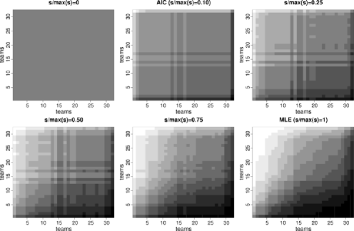
Figure 2: NFL regular season 2010–2011. Image plots illustrating several stages of the nonadaptive ranking lasso path. From top-left to bottom-right, images correspond to decreasing level of grouping, that is, increasing values of the relative bound s$/$max(s). The rows and the columns correspond to the teams sorted in decreasing order of their maximum likelihood estimated ability. The pixel of position (row${}={}$r, column${}={}$c) corresponds to the probability that team r wins against team c in a match played on a neutral field. Darker pixels correspond to higher probabilities of victory for the teams on the row.

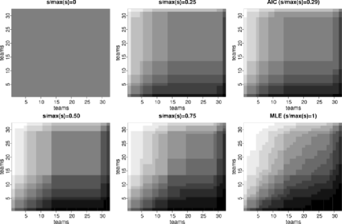
Figure 3: NFL regular season 2010–2011. Image plots illustrating several stages of the adaptive ranking lasso path. From top-left to bottom-right, images correspond to decreasing level of grouping, that is, increasing values of the relative bound s$/$max(s). The rows and the columns correspond to the teams sorted in decreasing order of their maximum likelihood estimated ability. The pixel of position (row${}={}$r, column${}={}$c) corresponds to the probability that team r wins against team c in a match played on a neutral field. Darker pixels correspond to higher probabilities of victory for the teams on the row.

These drawbacks are fixed by relying on the adaptive version designed to protect “true” large differences between abilities; see the path displayed in the right panel of Figure 1.

A useful visualization of the differences between the nonadaptive and the adaptive solutions is given in Figures 2 and 3. The image plots are constructed as follows. The rows and the columns correspond to the teams sorted in decreasing order of their maximum likelihood estimated ability, as in Table 1. For each image, the pixel of position $(r,c)$ is the probability that the team in row $r$ beats the team in column $c$ in a match played on a neutral field (no home effect),

$$\operatorname{pr}(Y_{rc}=1)=\frac{\exp(\hat{\mu}_{\lambda,r}-\hat{\mu}_{\lambda,c})}{1+\exp(\hat{\mu}_{\lambda,r}-\hat{\mu}_{\lambda,c})},\qquad r,c=1,\ldots,k.$$

Hence, the diagonal of the image is constant and equal to $0.5$. Higher values of the probabilities $\operatorname{pr}(Y_{rc}=1)$ correspond to colors shading off into dark. Figure 2 reports the image plots for several stages of the nonadaptive ranking lasso path, from the complete shrinkage ($s=0$) with all teams classified into the same group and thus the probability of victory in any match is $0.5$, the toss of a coin, to the maximum likelihood fit. The corresponding image plots for the adaptive fit are shown in Figure 3.

The comparison of the image plots in the two figures provides a clear illustration of the differences of the clustering process when adaptive weights are employed. Groups formed by the adaptive ranking lasso (Figure 3) are visualized by smooth blocks formed by spatially contiguous pixels, thus preserving the maximum likelihood ranking order. This is a consequence of the consistency of the adaptive lasso estimation method which assures that, for a sufficiently large tournament, the sign of the difference between maximum likelihood and adaptive ranking estimated abilities is the same. Vice versa, the image plots of the nonadaptive ranking lasso (Figure 2) have several spots because teams are frequently classified in different groups with respect to their closer neighbors.

Table 2: NFL regular season 2010–2011. Estimated probabilities of victory for the home team with corresponding 90% bias corrected percentile bootstrap confidence intervals for matches the Atlanta Falcons vs the Baltimore Ravens (home) and the Kansas City Chiefs vs the New England Patriots (home)

	Atlanta vs Baltimore	Kansas City vs New England
Method	est. (90% c.i.)	est. (90% c.i.)
MLE	0.56 (0.09, 0.90)	0.96 (0.75, 0.99)
AIC	0.56 (0.32, 0.81)	0.87 (0.76, 1.00)
BIC	0.56 (0.50, 0.84)	0.82 (0.78, 1.00)
Hybrid AIC	0.58 (0.15, 0.91)	0.97 (0.79, 0.99)
Hybrid BIC	0.58 (0.13, 0.93)	0.97 (0.83, 1.00)

We now move to the interpretation of the adaptive solution reported in Table 1, columns 4–7. AIC selects $9$ groups, while, as expected, BIC supports a sparser solution with $7$ groups. Both criteria agree in placing the New England Patriots on a single-team top group, followed by a group formed by the Atlanta Falcons, the Baltimore Ravens and the Pittsburgh Steelers. Differences between the two criteria regard the middle and the bottom part of the ranking. For example, AIC suggests that the Tampa Bay Buccaneers and the Philadelphia Eagles do better than the New York Giants, while BIC places these three teams in the same group together with the Indianapolis Colts and the Miami Dolphins. Clearly, the abilities estimated by the adaptive ranking lasso (columns 4–5 in Table 1) are considerably shrunken toward zero with respect to the maximum likelihood estimates. On the other hand, the hybrid adaptive ranking lasso method (columns 6–7 in Table 1) individuates the same groups but with estimated abilities that have the same extent of the maximum likelihood estimates.

The uncertainty of the estimated abilities is evaluated by parametric bootstrap with $1000$ replications. Table 2 reports the estimated probability of victory of the home teams in the matches Atlanta vs Baltimore played at Baltimore and Kansas City vs New England played at the home of the New England Patriots. These two matches were chosen to illustrate the behavior of the various estimation methods when the match involves teams with similar ability—Atlanta and Baltimore—or with large difference—Kansas City and New England. Similar results were obtained for the other matches.

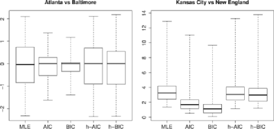
Figure 4: NFL regular season 2010–2011. Left panel: boxplots of the sample distributions of the estimated difference of abilities for the match between the Atlanta Falcons and the Baltimore Ravens (home) when the true model parameters correspond to the maximum likelihood estimates. The boxplots correspond to estimates by maximum likelihood (MLE), adaptive ranking lasso with AIC and BIC selection and hybrid adaptive ranking lasso/maximum likelihood with AIC (h-AIC) and BIC (h-BIC) selection. Right panel: boxplots of the sample distributions of the estimated difference of abilities for the match between the Kansas City Chiefs and the New England Patriots (home).

We start the discussion from the match between the Atlanta Falcons and the Baltimore Ravens. The maximum likelihood estimated probability that the Baltimore Ravens win is $\exp(1.75-1.82+0.32)/\{1+\exp(1.75-1.82+0.32)\}=0.56$. The adaptive ranking lasso method with either AIC and BIC selection attributes the same ability to the two teams. The 90% confidence interval for the victory of Baltimore based on maximum likelihood is very wide, being equal to $(0.09,0.90)$. Adaptive lasso bias-corrected percentile bootstrap confidence intervals are much shorter: $(0.32,0.81)$ with AIC selection and $(0.50,0.84)$ with BIC selection. Instead, hybrid adaptive ranking lasso confidence intervals are only slightly shorter than the maximum likelihood confidence interval.

In order to provide insights into the lengths of these confidence intervals, we estimated the sample distribution of the difference of the estimated abilities of Atlanta and Baltimore according to the various estimation methods assuming that the maximum likelihood estimate is the true model parameter. The above sample distributions are estimated with $1000$ Monte Carlo simulations and summarized by the boxplots in the left panel of Figure 4. Since the difference of the maximum likelihood estimated abilities for the two teams is close to zero, $1.75-1.82=-0.07$, the adaptive ranking lasso estimators have small biases with either AIC and BIC selection. Furthermore, the shrinkage effect yields a significant reduction in the variability of the adaptive ranking lasso estimators with respect to maximum likelihood estimators, as shown by the much smaller height of the boxes in Figure 4. Instead, the distributions of the hybrid adaptive ranking lasso estimators are very similar to the distribution of the maximum likelihood estimators.

The second match is played by the Kansas City Chiefs on the home field of the New England Patriots. The difference between the abilities of these two teams is very large. Indeed, the maximum likelihood estimate of the probability of New England victory is $0.96$. The adaptive ranking lasso is somehow more cautious with an estimated probability of wins equal to $0.87$ and $0.82$ according to AIC and BIC selections, respectively. The hybrid adaptive ranking lasso gives estimated probability of victory for New England that is essentially identical to maximum likelihood. However, the interesting aspect is that, despite the difference between the estimated probabilities of victory with maximum likelihood and adaptive ranking lasso, the bias-corrected confidence intervals are almost identical.

Again, insights into these confidence intervals come from the sample distribution of the differences of the estimated abilities assuming that the maximum likelihood estimate corresponds to the true model parameter. Boxplots reported in the right panel of Figure 4 show that in this case adaptive ranking lasso estimators are significantly biased toward zero with respect to maximum likelihood and hybrid adaptive ranking lasso estimators. More interestingly, the height of the boxes of all the five different estimators is rather similar. Accordingly, bias-corrected bootstrap percentile confidence intervals for the adaptive ranking lasso estimators are quite similar to those based on maximum likelihood and hybrid adaptive ranking lasso.

The overall conclusion is that if we compare two teams with close ability, then the shrinkage of the adaptive ranking lasso provides a sensible reduction in variability and thus shorter confidence intervals for the result of the match. Vice versa, if the ability of two teams is sensibly different, then the adaptive weights allow to obtain confidence intervals that are essentially equivalent to those obtained by maximum likelihood. Furthermore, the hybrid method does not seem particularly convenient in this context because it resembles maximum likelihood too closely.

These conclusions are coherent with the predictive performance of the various estimators discussed in the next section.

4.1 Predictive performance

We compare the predictive performance of the hybrid and the nonhybrid adaptive ranking lasso by repeating the following cross-validation exercise $100$ times:

form the training set by random sampling without replacing half the matches in the season;

determine the estimates of model parameters using the matches in the training set;

compute a predictive fit statistic summed over the remaining matches (the validation set).

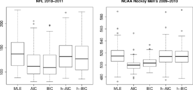
Figure 5: Boxplots of the cross-validated negative log-likelihoods computed at maximum likelihood (MLE) estimates, adaptive ranking lasso estimates with AIC and BIC selection and hybrid adaptive ranking lasso/maximum likelihood estimates with AIC (h-AIC) and BIC (h-BIC) selection. Left panel corresponds to the NFL regular season 2010–2011, right panel to the NCAA College Hockey Men’s Division I 2009–2010.

As a summary of the forecast’s quality in each cross-validation, we consider the negative of the log-likelihood computed with the matches in the validation set and model parameters estimated with the matches in the training set. This choice is, up to a constant term, equivalent to the Kullback–Leibler divergence and thus consistent with information model selection criteria.

The left panel of Figure 5 displays the boxplots of the $100$ negative log-likelihoods (one for each replication of the cross-validation experiment) and Table 3 provides some summaries. As clearly shown by boxplots, the shrinkage of adaptive ranking lasso estimates provides a sensible improvement of the prediction quality with respect to maximum likelihood predictions. Summaries in Table 3 show that the AIC selection improves on maximum likelihood of about $15\%$ in mean and $19\%$ in median, while BIC selection does slightly better with an improvement of $16\%$ in mean and $20\%$ in median. Predictions based on the hybrid ranking lasso, instead, are comparable to those based on maximum likelihood estimates with a very limited improvement. In summary, this prediction exercise supports adaptive ranking lasso without refitting because the method is able to create groups and at the same time increase the quality of predictions.

Finally, we observe that the percentage of matches which are predicted better than coin tossing is about $60\%$ for all methods.

Table 3: NFL regular season 2010–2011. Means and medians of the cross-validated negative log-likelihoods and percentage of predictions of the correct result which are better than coin tossing ($\succ\mathrm{coin}$)

		Lasso		Hybrid
	MLE	AIC	BIC	AIC	BIC
Mean	$139.90$	$119.10$	$117.20$	$135.20$	$131.60$
Median	$137.30$	$111.70$	$109.30$	$131.90$	$127.30$
$\succ$ coin	$0.59$	$0.60$	$0.58$	$0.60$	$0.60$

5 Handling ties

We focused on the analysis of sports not allowing ties or with no ties observed, as in the NFL example. However, there are a number of sports where ties are allowed and occur with a certain frequency. The ranking lasso analysis of these sport tournaments follows the lines outlined along the paper, with the only difference that we need to modify the Bradley–Terry model so as to handle ties. The match outcome becomes a three-level ordinal variable that can be arbitrarily coded as

$$Y_{ijr}=\cases{2,&\quad$\mbox{if team $i$ defeats team $j$,}$\vspace*{2pt}\cr 1,&\quad$\mbox{if teams $i$ and $j$ tied,}$\vspace*{2pt}\cr 0,&\quad$\mbox{if team $i$ is defeated by team $j$.}$}$$

Matches with ties can be modeled by some ordinal-valued extension of the Bradley–Terry model. For example, one may consider a cumulative link Bradley–Terry model [Agresti (2010)]

$$\operatorname{pr}(Y_{ijr}\leq y_{ijr})=\frac{\exp(\delta_{y_{ijr}}+h_{ijr}\tau+\mu_{i}-\mu_{j})}{1+\exp(\delta_{y_{ijr}}+h_{ijr}\tau+\mu_{i}-\mu_{j})},$$

where $-\infty\leq\delta_{0}\leq\delta_{1}\leq\delta_{2}\equiv+\infty$ are cutpoint parameters, while the other quantities are defined as in the previous sections of this paper.

Model identifiability now requires an additional contrast. Indeed, for every match played on a neutral field we must ensure that the probability that team $i$ defeats team $j$ is equal to the probability that team $j$ is defeated by team $i$. This condition is guaranteed when $\delta_{0}=-\delta_{1}$. If no tie is observed, or if it is not allowed by sport rules, then categories $1$ and $2$ are collapsed, $\delta_{0}=\delta_{1}=0,$ and the model reduces to the standard Bradley–Terry model.

5.1 NCAA college hockey men’s division I 2009–2010

We employ the ranking lasso with ties to the regular season of the NCAA College Hockey Men’s Division I 2009–2010. This tournament comprises $58$ teams partitioned in six conferences, namely, the Central Collegiate Hockey Association, the Western Collegiate Hockey Association, the Hockey East, the College Hockey America, the ECAC Hockey and the Atlantic Hockey. The composite schedule includes within and between conference games. The total number of matches is $1083$. The tournament design is highly incomplete. Indeed, about $73.3\%$ of the $(58\cdot 57)/2=1653$ possible matches are not played, $6.8\%$ are played just once, $10.5\%$ twice and the remaining $9.4\%$ are played three or more times, with seven matches ($0.4\%$) repeated even seven times. The tournament is also unbalanced with the total number of matches per team varying from $31$ to $43$.

Hockey matches may end with ties and these occur with a nonnegligible frequency. In the regular season of the NCAA College Hockey Men’s Division I 2009–2010 there were $125$ ties out of the $1083$ matches, that is, $11.5\%$ of the matches. The home effect also seems quite relevant because $54.8\%$ of the matches were won by the home team, $11.6\%$ ended with a tie and $33.5\%$ were won by the visitors. These numbers do not count the $69$ matches played on a neutral field.

At the end of the season, sixteen teams are qualified for the four regional semifinals. Hence, the four regional champions compete in the Frozen Four for the national championship. The matches’ results are available in the data frame icehockey through the R package BradleyTerry2 [Turner and Firth (2012)]. As reported in the help pages of this package, the NCAA selection system has been the source of several criticisms because there is no agreement that it correctly accounts for the highly irregular design of the tournament. The ranking based on the Bradley–Terry model is seen as a sensible alternative to the NCAA selection mechanism.

The maximum likelihood estimates of the home field parameter $\tau$ and the threshold parameter $\delta_{1}$ are both strongly significant: $\hat{\tau}^{(\mathrm{mle})}=0.402$ with a standard error of $0.066$ and $\hat{\delta}_{1}^{(\mathrm{mle})}=0.288$ with a standard error of $0.024$. The maximum likelihood estimates of the teams abilities, under the sum contrast, are listed in the third column of Table 4. According to the maximum likelihood fit of the Bradley–Terry model with ties, the best team is Denver, followed by Miami (Ohio), Wisconsin and Boston College. The last two teams were the finalists of the national championship won by Boston College on April 4, 2010.

Table 4: American College Hockey Men’s Division I composite schedule 2009–2010. For each team, the table displays the record and the ability estimated by maximum likelihood (MLE), by adaptive ranking lasso (lasso) and by hybrid adaptive ranking lasso/maximum likelihood (hybrid). Results are shown with both AIC and BIC model selection. Teams qualified for NCAA Regional semifinals are marked by symbol ^†

			Lasso		Hybrid
Teams	Record	MLE	AIC	BIC	AIC	BIC
Denver†	27–4–9	$1.65$	$0.58$	$0.41$	$1.38$	$1.36$
Miami (Ohio)†	27–7–7	$1.60$	$0.58$	$0.41$	$1.38$	$1.36$
Wisconsin†	25–4–10	$1.53$	$0.58$	$0.41$	$1.38$	$1.36$
Boston College†	25–3–10	$1.43$	$0.58$	$0.41$	$1.38$	$1.36$
North Dakota†	25–5–12	$1.37$	$0.58$	$0.41$	$1.38$	$1.36$
St Cloud State†	23–5–13	$1.10$	$0.18$	$0.09$	$0.60$	$0.56$
New Hampshire†	17–7–13	$0.89$	$0.18$	$0.09$	$0.60$	$0.56$
Minnesota Duluth	22–1–17	$0.87$	$0.18$	$0.09$	$0.60$	$0.56$
Bemidji State†	23–4–9	$0.87$	$0.18$	$0.09$	$0.60$	$0.56$
Michigan†	25–1–17	$0.86$	$0.18$	$0.09$	$0.60$	$0.56$
Colorado College	19–3–17	$0.86$	$0.18$	$0.09$	$0.60$	$0.56$
Northern Michigan†	20–8–12	$0.81$	$0.18$	$0.09$	$0.60$	$0.56$
Vermont†	17–7–14	$0.79$	$0.18$	$0.09$	$0.60$	$0.56$
Ferris State	21–6–13	$0.77$	$0.18$	$0.09$	$0.60$	$0.56$
Minnesota	18–2–19	$0.74$	$0.18$	$0.09$	$0.60$	$0.56$
Alaska†	18–9–11	$0.74$	$0.18$	$0.09$	$0.60$	$0.56$
Cornell†	21–4–8	$0.73$	$0.18$	$0.09$	$0.60$	$0.56$
Maine	19–3–17	$0.66$	$0.18$	$0.09$	$0.60$	$0.56$
UMass-Lowell	19–4–16	$0.64$	$0.18$	$0.09$	$0.60$	$0.56$
Yale†	20–3–9	$0.60$	$0.18$	$0.09$	$0.60$	$0.56$
Michigan State	19–6–13	$0.58$	$0.18$	$0.09$	$0.60$	$0.56$
Boston University	18–3–17	$0.57$	$0.18$	$0.09$	$0.60$	$0.56$
Nebraska-Omaha	20–6–16	$0.57$	$0.18$	$0.09$	$0.60$	$0.56$
Massachusetts	18–0–18	$0.56$	$0.18$	$0.09$	$0.60$	$0.56$
Northeastern	16–2–16	$0.51$	$0.18$	$0.09$	$0.60$	$0.56$
Ohio State	15–6–18	$0.45$	$0.18$	$0.09$	$0.60$	$0.56$
Minnesota State	16–3–20	$0.43$	$0.18$	$0.09$	$0.60$	$0.56$
Merrimack	16–2–19	$0.40$	$0.18$	$0.09$	$0.60$	$0.56$
Union (New York)	21–6–12	$0.29$	$0.18$	$0.09$	$0.60$	$0.56$
Notre Dame	13–8–17	$0.16$	$0.10$	$0.09$	$0.10$	$0.56$
Lake Superior	15–5–18	$0.15$	$0.10$	$0.09$	$0.10$	$0.56$
Alaska Anchorage	11–2–23	$-0.00$	$-0.09$	$-0.04$	$-0.34$	$-0.34$
St. Lawrence	19–7–16	$-0.17$	$-0.09$	$-0.04$	$-0.34$	$-0.34$
Providence	10–4–20	$-0.19$	$-0.09$	$-0.04$	$-0.34$	$-0.34$
Rensselaer	18–4–17	$-0.20$	$-0.09$	$-0.04$	$-0.34$	$-0.34$
Quinnipiac	20–2–18	$-0.24$	$-0.09$	$-0.04$	$-0.34$	$-0.34$
Western Michigan	8–8–20	$-0.24$	$-0.09$	$-0.04$	$-0.34$	$-0.34$
Colgate	15–6–15	$-0.34$	$-0.09$	$-0.04$	$-0.34$	$-0.34$

Table 4: (Continued)

			Lasso		Hybrid
Teams	Record	MLE	AIC	BIC	AIC	BIC
Rochester Institute of Technology†	26–1–11	$-0.39$	$-0.09$	$-0.04$	$-0.34$	$-0.34$
Alabama-Huntsville†	12–3–17	$-0.49$	$-0.09$	$-0.04$	$-0.34$	$-0.34$
Robert Morris	10–6–19	$-0.50$	$-0.09$	$-0.04$	$-0.34$	$-0.34$
Niagara	12–4–20	$-0.51$	$-0.09$	$-0.04$	$-0.34$	$-0.34$
Princeton	12–3–16	$-0.56$	$-0.09$	$-0.04$	$-0.34$	$-0.34$
Brown	13–4–20	$-0.61$	$-0.09$	$-0.04$	$-0.34$	$-0.34$
Bowling Green	5–6–25	$-0.76$	$-0.25$	$-0.10$	$-0.93$	$-0.92$
Sacred Heart	21–4–13	$-0.80$	$-0.09$	$-0.04$	$-0.34$	$-0.34$
Harvard	9–3–21	$-0.89$	$-0.25$	$-0.10$	$-0.93$	$-0.92$
Dartmouth	10–3–19	$-0.89$	$-0.25$	$-0.10$	$-0.93$	$-0.92$
Michigan Tech	5–1–30	$-1.03$	$-0.42$	$-0.24$	$-1.30$	$-1.30$
Clarkson	9–4–24	$-1.06$	$-0.42$	$-0.24$	$-1.30$	$-1.30$
Air Force	16–6–15	$-1.27$	$-0.25$	$-0.10$	$-0.93$	$-0.92$
Canisius	17–5–15	$-1.31$	$-0.25$	$-0.10$	$-0.93$	$-0.92$
Mercyhurst	15–3–20	$-1.59$	$-0.42$	$-0.24$	$-1.30$	$-1.30$
Army	11–7–18	$-1.60$	$-0.42$	$-0.24$	$-1.30$	$-1.30$
Holy Cross	12–6–19	$-1.71$	$-0.42$	$-0.24$	$-1.30$	$-1.30$
Bentley	12–4–19	$-1.78$	$-0.42$	$-0.24$	$-1.30$	$-1.30$
Connecticut	7–3–27	$-2.44$	$-1.17$	$-0.97$	$-2.19$	$-2.18$
American International	5–4–24	$-2.60$	$-1.17$	$-0.97$	$-2.19$	$-2.18$

Adaptive ranking lasso estimates of team abilities with or without refitting are listed in columns from four to seven of Table 4. AIC selects seven groups with a top group formed by the five teams with higher maximum likelihood estimates, namely, Denver, Miami, Wisconsin, Boston College and North Dakota. BIC instead suggests a slightly sparser solution with six groups. The only difference between AIC and BIC is that the latter rates Lake Superior and Alaska Anchorage at the same level of the preceding group in the AIC ranking.

The rankings obtained with the adaptive lasso penalization differ from the maximum likelihood ranking for a few teams at the bottom of the ranking. This result is not surprising. Both maximum likelihood and adaptive ranking lasso yield consistent estimation of teams’ abilities and, thus, they are expected to converge to the same ranking for sufficiently large tournaments, but for a finite tournament differences between the two rankings may occur. Given the strong incompleteness of the NCAA hockey tournament, the few observed differences between the two rankings are reasonable.

The predictive performance of the adaptive ranking lasso with the NCAA hockey tournament data is evaluated by the same cross-validation exercise previously used for the NFL example, as described at the beginning of Section 4.1. The right panel of Figure 5 displays the boxplots of the cross-validated negative log-likelihoods computed at the various estimators. The figure illustrates the outstanding predictive performance of the adaptive ranking lasso which largely outperforms predictions based on maximum likelihood. Differently from the previously analyzed NFL example, the larger number of teams and the strong irregularity of the tournament makes more evident the usefulness of the grouping effect induced by the lasso. Furthermore, the results strongly support the selection of the lasso penalty by AIC, while in the NFL application, predictions based on AIC and BIC were essentially of the same quality.

6 Conclusions

Lasso and its many variants have provided successful solutions to model selection in a variety of high-dimensional problems. In this paper we suggested a further use of the lasso ideas in the context of ranking contestants participating in a tournament. We showed how a generalized fused lasso penalty can be used for enhancing rankings derived from paired comparison models. The proposed adaptive ranking lasso method produces ranking in groups in a way that teams with similar ability are shrunk to the same common level.

Uncertainty of ranking lasso estimates can be evaluated by means of a parametric bootstrap. Our results support the idea that, as expected, the lasso-based estimates are more precise with respect to maximum likelihood estimates, in particular, when the true abilities of two teams are equal or nearly equal.

Lasso and other shrinkage methods are often motivated by superior predictive performance with respect to standard maximum likelihood. This is also the case of the proposed adaptive ranking lasso method. An empirical study suggests that ranking in groups induced by the adaptive ranking lasso produces forecasts of future matches whose quality is sensibly better than predictions based on maximum likelihood.

Although this paper is addressed to sport tournaments, we think that the discussed methodology can be of interest in many other ambits where rankings have to be derived from preference data. Further, the results in this paper can also be of interest because they highlight the benefits of adaptive versions of the lasso method as suggested by Zou (2006).

References

- Agresti (2010) {bbook}[mr] \bauthor\bsnmAgresti, \bfnmAlan\binitsA. (\byear2010). \btitleAnalysis of Ordinal Categorical Data, \bedition2nd ed. \bpublisherWiley, \blocationHoboken, NJ. \bidmr=2742515 \bptokimsref \endbibitem
- Böckenholt (2006) {barticle}[mr] \bauthor\bsnmBöckenholt, \bfnmUlf\binitsU. (\byear2006). \btitleThurstonian-based analyses: Past, present, and future utilities. \bjournalPsychometrika \bvolume71 \bpages615–629. \biddoi=10.1007/s11336-006-1598-5, issn=0033-3123, mr=2312235 \bptokimsref \endbibitem
- Bondell and Reich (2009) {barticle}[mr] \bauthor\bsnmBondell, \bfnmHoward D.\binitsH. D. and \bauthor\bsnmReich, \bfnmBrian J.\binitsB. J. (\byear2009). \btitleSimultaneous factor selection and collapsing levels in ANOVA. \bjournalBiometrics \bvolume65 \bpages169–177. \biddoi=10.1111/j.1541-0420.2008.01061.x, issn=0006-341X, mr=2665858 \bptokimsref \endbibitem
- Bradley and Terry (1952) {barticle}[mr] \bauthor\bsnmBradley, \bfnmRalph Allan\binitsR. A. and \bauthor\bsnmTerry, \bfnmMilton E.\binitsM. E. (\byear1952). \btitleRank analysis of incomplete block designs. I. The method of paired comparisons. \bjournalBiometrika \bvolume39 \bpages324–345. \bidissn=0006-3444, mr=0070925 \bptokimsref \endbibitem
- Candes and Tao (2007) {barticle}[mr] \bauthor\bsnmCandes, \bfnmEmmanuel\binitsE. and \bauthor\bsnmTao, \bfnmTerence\binitsT. (\byear2007). \btitleThe Dantzig selector: Statistical estimation when is much larger than . \bjournalAnn. Statist. \bvolume35 \bpages2313–2351. \biddoi=10.1214/009053606000001523, issn=0090-5364, mr=2382644 \bptokimsref \endbibitem
- Cattelan (2012) {barticle}[auto:STB—2012/09/03—07:24:02] \bauthor\bsnmCattelan, \bfnmM.\binitsM. (\byear2012). \btitleModels for paired comparison data: A review with emphasis on dependent data. \bjournalStatistical Science \bvolume27 \bpages412–433. \bptokimsref \endbibitem
- Chatterjee and Lahiri (2011) {barticle}[mr] \bauthor\bsnmChatterjee, \bfnmA.\binitsA. and \bauthor\bsnmLahiri, \bfnmS. N.\binitsS. N. (\byear2011). \btitleBootstrapping lasso estimators. \bjournalJ. Amer. Statist. Assoc. \bvolume106 \bpages608–625. \biddoi=10.1198/jasa.2011.tm10159, issn=0162-1459, mr=2847974 \bptokimsref \endbibitem
- Chen and Chen (2008) {barticle}[mr] \bauthor\bsnmChen, \bfnmJiahua\binitsJ. and \bauthor\bsnmChen, \bfnmZehua\binitsZ. (\byear2008). \btitleExtended Bayesian information criteria for model selection with large model spaces. \bjournalBiometrika \bvolume95 \bpages759–771. \biddoi=10.1093/biomet/asn034, issn=0006-3444, mr=2443189 \bptokimsref \endbibitem
- Donoho (1995) {barticle}[mr] \bauthor\bsnmDonoho, \bfnmDavid L.\binitsD. L. (\byear1995). \btitleDe-noising by soft-thresholding. \bjournalIEEE Trans. Inform. Theory \bvolume41 \bpages613–627. \biddoi=10.1109/18.382009, issn=0018-9448, mr=1331258 \bptokimsref \endbibitem
- Efron (1987) {barticle}[mr] \bauthor\bsnmEfron, \bfnmBradley\binitsB. (\byear1987). \btitleBetter bootstrap confidence intervals. \bjournalJ. Amer. Statist. Assoc. \bvolume82 \bpages171–185. \bidissn=0162-1459 \bptnotecheck related\bptokimsref \endbibitem
- Efron et al. (2004) {barticle}[mr] \bauthor\bsnmEfron, \bfnmBradley\binitsB., \bauthor\bsnmHastie, \bfnmTrevor\binitsT., \bauthor\bsnmJohnstone, \bfnmIain\binitsI. and \bauthor\bsnmTibshirani, \bfnmRobert\binitsR. (\byear2004). \btitleLeast angle regression. \bjournalAnn. Statist. \bvolume32 \bpages407–499. \biddoi=10.1214/009053604000000067, issn=0090-5364, mr=2060166 \bptnotecheck related\bptokimsref \endbibitem
- Fahrmeir and Tutz (1994) {barticle}[auto:STB—2012/09/03—07:24:02] \bauthor\bsnmFahrmeir, \bfnmL.\binitsL. and \bauthor\bsnmTutz, \bfnmG.\binitsG. (\byear1994). \btitleDynamic stochastic models for time-dependent ordered paired comparison systems. \bjournalJ. Amer. Statist. Assoc. \bvolume89 \bpages1438–1449. \bptokimsref \endbibitem
- Fan and Li (2001) {barticle}[mr] \bauthor\bsnmFan, \bfnmJianqing\binitsJ. and \bauthor\bsnmLi, \bfnmRunze\binitsR. (\byear2001). \btitleVariable selection via nonconcave penalized likelihood and its oracle properties. \bjournalJ. Amer. Statist. Assoc. \bvolume96 \bpages1348–1360. \biddoi=10.1198/016214501753382273, issn=0162-1459, mr=1946581 \bptokimsref \endbibitem
- Gertheiss and Tutz (2010) {barticle}[mr] \bauthor\bsnmGertheiss, \bfnmJan\binitsJ. and \bauthor\bsnmTutz, \bfnmGerhard\binitsG. (\byear2010). \btitleSparse modeling of categorial explanatory variables. \bjournalAnn. Appl. Stat. \bvolume4 \bpages2150–2180. \biddoi=10.1214/10-AOAS355, issn=1932-6157, mr=2829951 \bptokimsref \endbibitem
- Glickman (1999) {barticle}[auto:STB—2012/09/03—07:24:02] \bauthor\bsnmGlickman, \bfnmM. E.\binitsM. E. (\byear1999). \btitleParameter estimation in large dynamic paired comparison experiments. \bjournalApplied Statistics \bvolume48 \bpages377–394. \bptokimsref \endbibitem
- Glickman (2001) {barticle}[mr] \bauthor\bsnmGlickman, \bfnmMark E.\binitsM. E. (\byear2001). \btitleDynamic paired comparison models with stochastic variances. \bjournalJ. Appl. Stat. \bvolume28 \bpages673–689. \biddoi=10.1080/02664760120059219, issn=0266-4763, mr=1862491 \bptokimsref \endbibitem
- Guo et al. (2010) {barticle}[mr] \bauthor\bsnmGuo, \bfnmJian\binitsJ., \bauthor\bsnmLevina, \bfnmElizaveta\binitsE., \bauthor\bsnmMichailidis, \bfnmGeorge\binitsG. and \bauthor\bsnmZhu, \bfnmJi\binitsJ. (\byear2010). \btitlePairwise variable selection for high-dimensional model-based clustering. \bjournalBiometrics \bvolume66 \bpages793–804. \biddoi=10.1111/j.1541-0420.2009.01341.x, issn=0006-341X, mr=2758215 \bptokimsref \endbibitem
- Hestenes (1969) {barticle}[mr] \bauthor\bsnmHestenes, \bfnmMagnus R.\binitsM. R. (\byear1969). \btitleMultiplier and gradient methods. \bjournalJ. Optim. Theory Appl. \bvolume4 \bpages303–320. \bidissn=0022-3239, mr=0271809 \bptokimsref \endbibitem
- Joe (1990) {barticle}[mr] \bauthor\bsnmJoe, \bfnmHarry\binitsH. (\byear1990). \btitleExtended use of paired comparison models, with application to chess rankings. \bjournalJ. Roy. Statist. Soc. Ser. C \bvolume39 \bpages85–93. \biddoi=10.2307/2347814, issn=0035-9254, mr=1038891 \bptokimsref \endbibitem
- Knorr-Held (2000) {barticle}[auto:STB—2012/09/03—07:24:02] \bauthor\bsnmKnorr-Held, \bfnmL.\binitsL. (\byear2000). \btitleDynamic rating of sports teams. \bjournalThe Statistician \bvolume49 \bpages261–276. \bptokimsref \endbibitem
- Lian (2010) {bmisc}[auto:STB—2012/09/03—07:24:02] \bauthor\bsnmLian, \bfnmH.\binitsH. (\byear2010). \bhowpublishedA simple and efficient algorithm for fused lasso signal approximator with convex loss function. Available at arXiv:\arxivurl1005.5085. \bptokimsref \endbibitem
- Mease (2003) {barticle}[mr] \bauthor\bsnmMease, \bfnmDavid\binitsD. (\byear2003). \btitleA penalized maximum likelihood approach for the ranking of college football teams independent of victory margins. \bjournalAmer. Statist. \bvolume57 \bpages241–248. \biddoi=10.1198/0003130032396, issn=0003-1305, mr=2016258 \bptokimsref \endbibitem
- Nocedal and Wright (2006) {bbook}[mr] \bauthor\bsnmNocedal, \bfnmJorge\binitsJ. and \bauthor\bsnmWright, \bfnmStephen J.\binitsS. J. (\byear2006). \btitleNumerical Optimization, \bedition2nd ed. \bpublisherSpringer, \blocationNew York. \bidmr=2244940 \bptokimsref \endbibitem
- Powell (1969) {bincollection}[mr] \bauthor\bsnmPowell, \bfnmM. J. D.\binitsM. J. D. (\byear1969). \btitleA method for nonlinear constraints in minimization problems. In \bbooktitleOptimization (Sympos., Univ. Keele, Keele, 1968) \bpages283–298. \bpublisherAcademic Press, \blocationLondon. \bidmr=0272403 \bptokimsref \endbibitem
- R Development Core Team (2012) {bmisc}[auto:STB—2012/09/03—07:24:02] \borganizationR Development Core Team. (\byear2012). \bhowpublishedR: A Language and Environment for Statistical Computing. R Foundation for Statistical Computing, Vienna, Austria. Available at http://www.R-project.org/. \bptokimsref \endbibitem
- She (2010) {barticle}[mr] \bauthor\bsnmShe, \bfnmYiyuan\binitsY. (\byear2010). \btitleSparse regression with exact clustering. \bjournalElectron. J. Stat. \bvolume4 \bpages1055–1096. \biddoi=10.1214/10-EJS578, issn=1935-7524, mr=2727453 \bptokimsref \endbibitem
- Stern (2004) {barticle}[mr] \bauthor\bsnmStern, \bfnmHal S.\binitsH. S. (\byear2004). \btitleStatistics and the college football championship. \bjournalAmer. Statist. \bvolume58 \bpages179–195. \biddoi=10.1198/000313004X2098, issn=0003-1305, mr=2086363 \bptnotecheck related\bptokimsref \endbibitem
- Thurstone (1927) {barticle}[auto:STB—2012/09/03—07:24:02] \bauthor\bsnmThurstone, \bfnmL. L.\binitsL. L. (\byear1927). \btitleA law of comparative judgment. \bjournalPsychological Review \bvolume79 \bpages281–299. \bptokimsref \endbibitem
- Tibshirani (1996) {barticle}[mr] \bauthor\bsnmTibshirani, \bfnmRobert\binitsR. (\byear1996). \btitleRegression shrinkage and selection via the lasso. \bjournalJ. Roy. Statist. Soc. Ser. B \bvolume58 \bpages267–288. \bidissn=0035-9246, mr=1379242 \bptokimsref \endbibitem
- Tibshirani and Taylor (2011) {barticle}[mr] \bauthor\bsnmTibshirani, \bfnmRyan J.\binitsR. J. and \bauthor\bsnmTaylor, \bfnmJonathan\binitsJ. (\byear2011). \btitleThe solution path of the generalized lasso. \bjournalAnn. Statist. \bvolume39 \bpages1335–1371. \biddoi=10.1214/11-AOS878, issn=0090-5364, mr=2850205 \bptnotecheck year\bptokimsref \endbibitem
- Tibshirani et al. (2005) {barticle}[mr] \bauthor\bsnmTibshirani, \bfnmRobert\binitsR., \bauthor\bsnmSaunders, \bfnmMichael\binitsM., \bauthor\bsnmRosset, \bfnmSaharon\binitsS., \bauthor\bsnmZhu, \bfnmJi\binitsJ. and \bauthor\bsnmKnight, \bfnmKeith\binitsK. (\byear2005). \btitleSparsity and smoothness via the fused lasso. \bjournalJ. R. Stat. Soc. Ser. B Stat. Methodol. \bvolume67 \bpages91–108. \biddoi=10.1111/j.1467-9868.2005.00490.x, issn=1369-7412, mr=2136641 \bptokimsref \endbibitem
- Turner and Firth (2012) {barticle}[auto:STB—2012/09/03—07:24:02] \bauthor\bsnmTurner, \bfnmH.\binitsH. and \bauthor\bsnmFirth, \bfnmD.\binitsD. (\byear2012). \btitleBradley–Terry models in R: The BradleyTerry2 package. \bjournalJournal of Statistical Software \bvolume48 \bpages1–21. \bptokimsref \endbibitem
- Ye and Xie (2011) {barticle}[mr] \bauthor\bsnmYe, \bfnmGui-Bo\binitsG.-B. and \bauthor\bsnmXie, \bfnmXiaohui\binitsX. (\byear2011). \btitleSplit Bregman method for large scale fused Lasso. \bjournalComput. Statist. Data Anal. \bvolume55 \bpages1552–1569. \biddoi=10.1016/j.csda.2010.10.021, issn=0167-9473, mr=2748661 \bptokimsref \endbibitem
- Zou (2006) {barticle}[mr] \bauthor\bsnmZou, \bfnmHui\binitsH. (\byear2006). \btitleThe adaptive lasso and its oracle properties. \bjournalJ. Amer. Statist. Assoc. \bvolume101 \bpages1418–1429. \biddoi=10.1198/016214506000000735, issn=0162-1459, mr=2279469 \bptokimsref \endbibitem