The cluster ages experiment (CASE). V. Analysis of three eclipsing binaries in the globular cluster M4^∗

Abstract

We use photometric and spectroscopic observations of the eclipsing binaries V65, V66 and V69 in the field of the globular cluster M4 to derive masses, radii, and luminosities of their components. The orbital periods of these systems are 2.29, 8.11 and 48.19 d, respectively. The measured masses of the primary and secondary components ($M_{p}$ and $M_{s}$) are 0.8035$\pm$0.0086 and 0.6050$\pm$0.0044 M_⊙ for V65, 0.7842$\pm$0.0045 and 0.7443$\pm$0.0042 M_⊙ for V66, and 0.7665$\pm$0.0053 and 0.7278$\pm$0/0048 M_⊙ for V69. The measured radii ($R_{p}$ and $R_{s}$) are 1.147$\pm$0.010 and 0.6110$\pm$0.0092 R_⊙ for V66, 0.9347$\pm$0.0048 and 0.8298$\pm$0.0053 R_⊙ for V66, and 0.8655$\pm$0.0097 and 0.8074$\pm$0.0080 R_⊙ for V69. The orbits of V65 and V66 are circular, whereas that of V69 has an eccentricity of 0.38. Based on systemic velocities and relative proper motions, we show that all the three systems are members of the cluster. We find that the distance to M4 is 1.82$\pm$0.04 kpc - in good agreement with recent estimates based on entirely different methods. We compare the absolute parameters of V66 and V69 with two sets of theoretical isochrones in mass-radius and mass-luminosity diagrams, and for an assumed [Fe/H] = -1.20, [$\alpha$/Fe] = 0.4, and Y = 0.25 we find the most probable age of M4 to be between 11.2 and 11.3 Gyr. CMD-fitting with the same parameters yields an age close to, or slightly in excess of, 12 Gyr. However, considering the sources of uncertainty involved in CMD fitting, these two methods of age determination are not discrepant. Age and distance determinations can be further improved when infrared eclipse photometry is obtained.

Key words: binaries: close – binaries: spectroscopic – globular clusters: individual (M4) – stars: individual (V65-M4, V66-M4, V69-M4)

1 Introduction

Detached eclipsing double-line binaries (DEBs) are the primary source of the observational data concerning stellar masses and radii. When supplemented by luminosities derived from parallaxes, empirical relations between color and effective temperature, or fits to disentangled spectra, they enable fundamental tests of stellar evolution models. For many field Population I binaries with components at solar mass or larger, modern high accuracy measurements of masses, radii and luminosities are in general agreement with theoretical predictions (see, for example, Lacy et al., 2005, 2008; Clausen et al., 2008). Similar encouraging results are obtained for binaries in the old open clusters NGC 188 (Meibom et al., 2009), NGC 2243 (Kaluzny et al., 2006), and NGC 6791 (Grundahl et al., 2008; Brogaard et al., 2011). On the other hand, the models seem to underestimate the radii of numerous K and M dwarfs in short-period binaries. Summaries of relevant recent measurements can be found for example in Blake et al. (2008), Torres et al. (2010), and Kraus et al. (2011).

The situation is less clear for Population II stars, for which only a very few DEBs with main-sequence components are known (Thompson et al., 2010), and there is an urgent need to locate and study such systems. Within the series Cluster AgeS Experiment (CASE), this is the second paper devoted to the study of globular-cluster DEBs with main-sequence or subgiant components. The general goal of CASE is to determine the basic stellar parameters (masses, luminosities, and radii) of the components of cluster binaries to a precision better than 1% in order to measure cluster ages and distances, and to test stellar evolution models (Kaluzny et al., 2005). The methods and assumptions we employ utilize basic and simple approaches, following the ideas of Paczyński (1997) and Thompson et al. (2001). Previous CASE papers analyzed blue straggler systems in $\omega$ Cen (Kaluzny et al., 2007a) and 47 Tuc (Kaluzny et al., 2007b), an SB1 binary in NGC 6397 (Kaluzny et al., 2008) and the binary V69-47 Tuc, which is an SB2 system with main-sequence components (Thompson et al., 2010).

The present paper is devoted to the analysis of three DEBs, V65, V66 and V69, all members of the globular cluster M4. We use radial velocity and photometric observations to determine accurate masses, luminosities, and radii of the components of these systems.

Section 2 describes the photometric observations and the determination of orbital ephemerides. Section 3 presents the spectroscopic observations and the radial-velocity measurements. The combined photometric and spectroscopic solutions for orbital elements and component parameters are obtained in Section 4, while the cluster membership of the three DEBs is discussed in Section 5. In Section 6, we compare the derived parameters to a selection of stellar evolution models, with an emphasis on estimating the age of the system. Finally, in Section 7 we summarize our findings.

2 Photometric observations

Our survey for eclipsing binaries in M4 began in July 1995 with a 2-week observational campaign at CTIO. We monitored the cluster in the $B$- and $V$-bands, using the 2K² TEK2 camera attached to the 0.9-m telescope. A single eclipse of V66 was detected, occurring on 1995 July 18 UT. The survey continued on the 1.0-m Swope telescope at Las Campanas Observatory (LCO) using five different CCD cameras (Ford, TEK3, SITe1, SITe2, and SITe3) over several seasons during the period 1996 - 2009. Most of the observations were obtained with the SITe3 camera, with a plate scale of 0.435 arcsec/pixel and a field size of 14.8$\times$22.8 arcmin². Some early results from this survey were presented in Kaluzny et al. (1997).

The first eclipses of V65 and V69 were detected on 1996 April 16 UT and 1996 April 21 UT, respectively. In the same year preliminary but reliable ephemerides for V65 and V66 were determined. A part of a secondary eclipse of V69 was observed on 1998 August 17 UT. However, because of the relatively long period for this system, the data were still insufficient to establish a unique ephemeris. An initial ephemeris was derived from constraints provided by substantial out-of-eclipse photometry performed in 1996 - 2005, and radial velocity observations obtained with the MIKE spectrograph on the Magellan Baade and Clay telescopes (see Section 3). From 1998 until 2009 we also observed our targets with the 2.5-m du Pont telescope at LCO equipped with the TEK5 2K² camera with a plate scale of 0.259 arcsec/pixel. Between 2001 and 2009, several eclipses were covered for V65 and V69, and some out-of-eclipse data were collected for V69. In all observing runs, on each telescope, the same $B$ and $V$ filters were used. Times of minima are presented in Tables 1, 2, and 3.

Linear ephemerides provide adequate fits to the photometric data for all three binaries, these are given by Equations (1). In the case of V65 and V66 the ephemerides were obtained from the moments of minima calculated from individual light curves. This procedure could not be applied to V69, as in only three eclipses both the descending and the ascending branch was observed. In the case of V69, the period was derived using the algorithm developed by Lafler & Kinmann (1965), and the moment of the primary eclipse was found from the phased light curve with an improved version of the method developed by Kwee & van Woerden (1956). For V65, only du Pont observations were used, reduced with the image subtraction technique. For V66, we also made use of photometry measured with profile fitting in images collected with the Swope and 0.9-m CTIO telescopes.

$$HJD^{\mathrm{V65}}_{\mathrm{min}} = 2449905.49577(43)+2.29304564(26)\times E$$

$$HJD^{\mathrm{V66}}_{\mathrm{min}} = 2449900.41965(26)+8.11130346(85)\times E$$ (1)

$$HJD^{\mathrm{V69}}_{\mathrm{min}} = 2450048.34890(14)+48.1882687(6)\times E$$

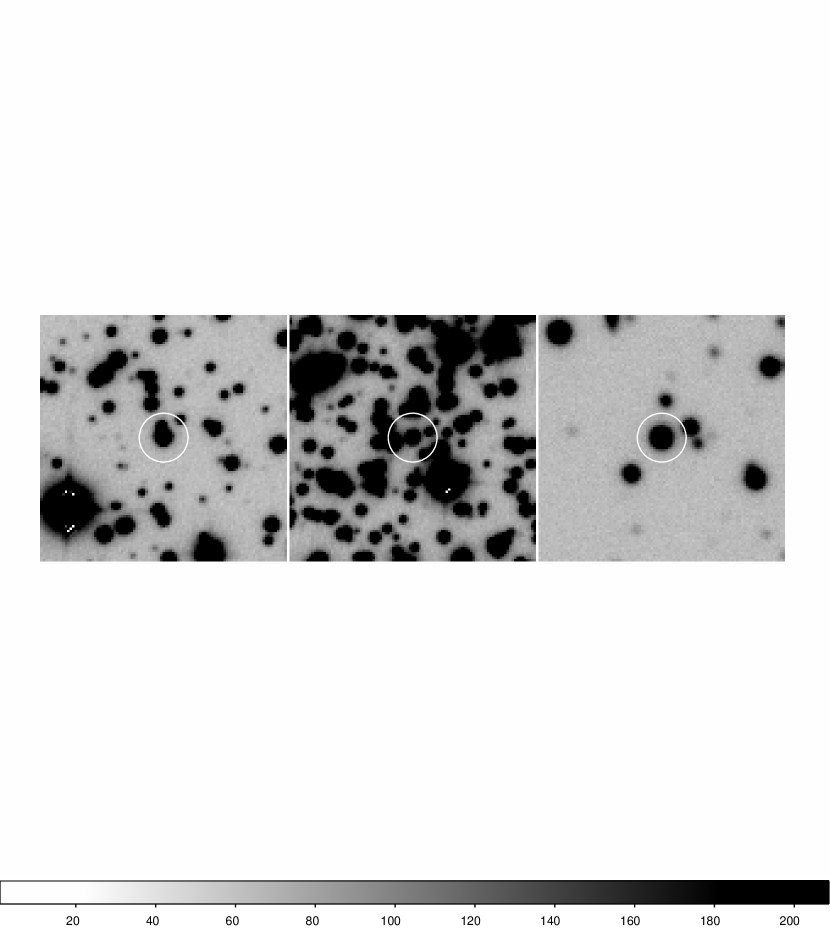
Figure 1: Finding charts for V65 (left), V66 (middle) and V69 (right). Each chart is 26″ on a side, and is oriented with north up and east to the left. The coordinates of the targets are given in Table 4.

Table 4 gives the equatorial coordinates of the three variables analysed in this paper. They are tied to the UCAC3 system (Zacharias et al., 2010) for V65 and V66 , and to the GSC-1.0 system (e.g. Lasker et al., 1990) for V69. Finding charts prepared from du Pont TEK5 $V$-band images are shown in Figure 1.

V65 is blended with two stars located at angular distances of 0.37″ and 0.57″. The variable is the brightest component of the blend. All three stars are included in ACS-HST HST F606W/F814W photometry published by Anderson et al. (2008), with star identification numbers 13362, 13372 (V65), and 13374. The HST photometry is listed in Table 5. We determined the rectangular coordinates of V65 and its two close visual companions on the reference image by transforming their positions from ACS/HST photometry of Anderson et al. (2008), and the presence of the companions was taken into account while extracting light curves of this binary. V66 is listed by Anderson et al. (2008) as star 5795. It does not suffer from any blending which could affect the ground based photometry. V69 is not present in any of the currently available HST images of M4. The object is located at an angular distance of 7.69′ from the center of the cluster, beyond the half-light radius of 4.33′ (Harris, 1996, 2010 edition). The du Pont images show no evidence of any unresolved visual companions to V69.

2.1 Light curves and calibration of photometry.

The $B$ and $V$ light curves of V65 and V66 were determined entirely from the du Pont data. They were extracted with the image subtraction technique, using methods and codes described in Kaluzny et al. (2010). In short, we used a combination of ISIS 2.1 (Alard & Lupton, 1998), Allstar/Daophot (Stetson, 1987) and Daogrow (Stetson, 1990) codes, supplemented with some IRAF¹ tasks. For these two variables, we also extracted light curves using profile fitting software to make sure that the image subtraction technique is free from systematic errors (in particular, we checked that the curves resulting from profile photometry and image subtraction have the same amplitudes). As expected, the scatter produced by the image subtraction technique was significantly smaller.

$B$ and $V$ light curves of V69 were obtained from the data collected with the Swope telescope and the SITe3 camera. The light curves were measured using profile fitting software since this variable is located in a sparsely populated field and image subtraction offers no advantage in comparison with the traditional profile photometry. We also collected a few frames containing V69 with the du Pont telescope and used these to measure the magnitude and color of this variable at maximum light. Observations Landolt (1992) photometric standards obtained with the du Pont telescope enabled us to transform the light curves of all three variables to the standard $BV$ system.

Full details of the procedure employed to perform the photometric measurements will be reported in a separate paper devoted to the photometry of other variables in M4 (Kaluzny et al., in preparation), along with the measurement of differential and global reddening in the field of the cluster. Table 6 lists magnitudes and colors of V65, V66 and V69 at maximum light, together with the reddening towards each of the variables. The errors include internal and external uncertainties, and the last column gives the total reddening as determined by Kaluzny et al. (in preparation; the reddening was found by comparing turnoff colors of M4 and the low-extinction cluster NGC 6362).

The light curve of V65 is unstable (see Figure 2). The fast rotation of the components, implied by the relatively short orbital period of 2.29 d, apparently induces a strong magnetic activity in at least one of the stars. A clear sign of such an activity is the X-ray emission: the system was listed by Bassa et al. (2004) as the X-ray source CX 30 with $L_{\rm x}=2.6\times 10^{29}$ erg s^-1. For the present analysis, we selected observations collected between 2008 June 07 and 2009 June 30. During that period the light curve was flat between the eclipses, the eclipses were symmetric (note the totality of the secondary eclipse), and the binary was brighter than in the other observing seasons. All these observations indicate that the magnetic activity of the system was significantly lower than during the other observing seasons.

The remaining two light curves are stable. While the eclipses of the star V66 are symmetric and separated by a half of the orbital period, the orbit of V69 is clearly eccentric, and the secondary eclipse occurs at phase 0.609. The final light curves adopted for the analysis of the three systems are shown in Figure 3.

3 Spectroscopic observations

The spectra were taken with the MIKE echelle spectrograph (Bernstein et al., 2003) on the Magellan Baade and Clay 6.5-m telescopes, using a 0.7″ slit, which provided a resolution R $\approx$40,000. A typical observation consisted of two 1800-second exposures of the target, flanking an exposure of a thorium-argon hollow-cathode lamp. A few of the exposures were shorter, depending on the observing conditions. The raw spectra were reduced with the pipeline software written by Dan Kelson, following the approach outlined in Kelson (2003). The IRAF package ECHELLE was used for the post-extraction processing. The velocities were measured using software based on the TODCOR algorithm (Zucker & Mazeh, 1994), kindly made available by Guillermo Torres. For velocity templates, we used synthetic echelle-resolution spectra from the library of Coelho et al. (2006). These were interpolated to the values of $\log g$ and $T_{eff}$ derived from the photometric solution (see Section 4) and assuming ${\rm[Fe/H]}=-1.2$ with an $\alpha$-element enhancement of 0.4 (Caretta et al., 2009; Dotter et al., 2010). The results of the velocity measurements are insensitive to minor changes in these parameters. The templates were Gaussian-smoothed to match the resolution of the observed spectra. In the case of V65, a rotational broadening was additionally applied.

For both V66 and V69, the cross-correlations with template spectra were performed independently on wavelength intervals 4120-4320 Å and 4350-4600 Å, covering the region of the MIKE blue spectra with the best signal-to-noise ratio while avoiding the H $\gamma$ line. The final velocities adopted for the analysis were obtained by averaging the results of these two measurements. In the case of V65, the spectrum was contaminated by one of the stars blended with the target (ID 13374 in Table 5), so that a three-dimensional extension of the original TODCOR algorithm (Zucker, Torres & Mazeh, 1995) had to be used. The cross-correlation was performed on the interval 4000-4840 Å to maximize the signal from the very faint secondary component. The second contaminating star (ID 13362 in Table 5), which is fainter and more distant on the sky from the target, was not detected in the velocity cross correlation functions.

The results of velocity measurements are presented in Tables 7, 8, and 9, which list heliocentric Julian dates at mid-exposure, velocities of the primary and secondary components, and orbital phases of the observations, calculated according to the ephemerides given by Equations (1). In the case of V65 the velocities of the contaminating star are also given. The observed velocity curves were fit with a nonlinear least squares solution, using code kindly made available by Guillermo Torres. Both the observed curves and the fitted ones are shown in Figure 4, and the derived orbital parameters are listed in Table 10, together with errors as returned by the fitting routine. Table 10 also lists the velocity standard deviations $\sigma_{p}$ and $\sigma_{s}$ of the orbital solution which are a measure of the precision of a single velocity measurement. In all cases, the fits adopted the periods and times of primary eclipse as given in Equations (1).

4 Light curve analysis and system parameters

The analysis of the light curves was performed with the PHOEBE implementation (Prša & Zwitter, 2005) of the Wilson-Devinney (WD) model (Wilson & Devinney, 1971; Wilson, 1979). The PHOEBE/WD package utilizes the Roche geometry to approximate the shapes of the stars, uses Kurucz model atmospheres, treats reflection effects in detail, and, most importantly, allows for the simultaneous analysis of $B$ and $V$ data. The resulting geometrical parameters are largely determined by the higher-quality $V$ data, while the $B$ data serves mainly to estimate of the luminosity ratio $L_{s}/L_{p}$ in that band. To find the best initial parameters for PHOEBE iterations, we solved for the $V$ data using the JKTEBOP code (Southworth et al., 2004, and references therein), which, unlike PHOEBE, can deal with a single light curve only, but it is capable of a robust search for the global minimum in the parameter space.

Before solving for the light curves, it was necessary to estimate the effective temperature of the primary, $T_{p}$. To that end, we used the $(B-V)$ and $E(B-V)$ values from Table 6, and the calibration of Casagrande et al. (2010). Apart from $T_{p}$, PHOEBE needs to be given a metallicity, albedo, and gravity darkening coefficient. The user also has to specify which limb darkening law is to be used. We adopted a metallicity of ${\rm[Fe/H]}=-1.20$ (see Section 3 and Section 6). Bolometric albedo and gravity darkening coefficients were set to values appropriate for stars with convective envelopes: $A=0.5$, and $g=0.32$ (we note that all three systems are well detached, so that effects of reflection and gravity only weakly affect their light curves). We used a linear approximation for the limb darkening. Theoretical limb darkening coefficients in the $BV$ bands were interpolated from the tables compiled by Claret (2000), using the jktld code.² The parameters of each binary were found iteratively according to the following procedure:

1. Solve for the velocity curve, as explained in Section 3. Find a preliminary solution of the $V$-light curve using JKTEBOP. Feed the obtained parameters into PHOEBE.

2. Solve for the light curves, fitting orbital inclination $i$, effective temperature of the secondary $T_{s}$, gravitational potentials at the surface of the primary $\Omega_{p}$ and the secondary $\Omega_{s}$, and relative luminosities $L^{B}_{s}/L^{B}_{p}$ and $L^{V}_{s}/L^{V}_{p}$ in $B$ and $V$ bands.

3. Based on the relative luminosities obtained in Step 3, calculate the $(B-V)_{0}$ index of the primary, and update $T_{p}$, using, as before, the calibrations of Casagrande et al. (2010).

4. Repeat steps 2 and 3 until iterations converge (i.e. until the last iterated corrections to the parameters became smaller than the formal errors of those parameters).

The eccentricity and argument of periastron for V69 were found from the velocity curve. We obtained a preliminary photometric solution in which they were allowed to vary, but since they changed by only 10% of the errors given in Table 10, we decided to keep them constant during proper iterations.

The residuals of the fits are shown in Figure 5 and the final values of the iterated parameters are given in Table 11. We checked that the luminosity ratios and relative radii of the components were practically insensitive to changes in effective temperature of the primary: $(L_{s}/L_{p})_{B}$, $(L_{s}/L_{p})_{V}$, $r_{s}$, and $r_{p}$, all changed by less than 0.3% for a $\pm$150 K change in $T_{p}$. The standard errors of the six parameters iterated upon by PHOEBE were found using a Monte Carlo procedure written in the PHOEBE-scripter, and similar to that outlined in the description of the JKTEBOP code (see Southworth et al., 2004, and references therein). Briefly, the procedure replaces the observed light curves $B_{o}$ and $V_{o}$ with the fitted ones $B_{f}$ and $V_{f}$, generates Gaussian perturbations $\delta B_{f}$ and $\delta V_{f}$ such that the standard deviation of the perturbation is equal to the standard deviation of the corresponding residuals shown in Figure 5, and performs PHOEBE iterations on $B_{f}+\delta B_{f}$ and $V_{f}+\delta V_{f}$. Each Monte Carlo run produced 15000 points. Examples of the Monte Carlo diagrams are shown in Figure 6. The combination of spectroscopic and photometric solutions yielded absolute parameters of the three DEBs which we list in Table 12. The measured masses of the primary and secondary components ($M_{p}$ and $M_{s}$) are 0.8035$\pm$0.0086 and 0.6050$\pm$0.0044 M_⊙ for V65, 0.7842$\pm$0.0045 and 0.7443$\pm$0.0042 M_⊙ for V66, and 0.7665$\pm$0053 and 0.7278$\pm$0/0048 M_⊙ for V69. The measured radii ($R_{p}$; $R_{s}$) are 1.1470$\pm$0.0104 and 0.6110$\pm$0.0092 R_⊙ for V66, 0.9347$\pm$0.0048 and 0.8298$\pm$0.0053 R_⊙ for V66, and 0.8655$\pm$0.0097 and 0.8074$\pm$0.0080 R_⊙ for V69. The measured accuracy of the mass determinations ranges from 0.6% for the primary of V66 to 1.1% for the secondary of V65. The measured accuracy of the radii determinations ranges from 0.5% for the primary of V66 to 1.5% for the secondary of V65. The location of the components on the CMD of M4 is shown in Figure 7. This CMD shows data for a 3.5$\times$3.5 arcmin² field whose center is located 1.4 arcmin from the center of the cluster. This field was chosen because it shows relatively uniform extinction. The photometry of all stars in Figure 7 (including the three DEBs) has been corrected for differential reddening (Kaluzny et al., in prep.). No attempt was made to remove nonmembers of M4.

5 Membership of the target binaries and the distance to M4

Upon averaging the subtracted images on a seasonal basis, we found no evidence of bipolar residuals at the positions of our targets. Such residuals are observed for objects with noticeable proper motions with respect to the surrounding stellar field (Eyer & Wozniak, 2001). Given the time base and the pixel scale of our images, we rule out motions in excess of 10 mas/y. Since on the proper-motion diagram of M4 most of the field stars are separated from the cluster population by more than 15 mas/y (Zloczewski, 2012), this is consistent with all the three targets being members of M4.

The radial velocity of M4 is equal to 70.29$\pm$0.07 km s^-1 (Sommariva et al., 2009), while the velocity dispersion is 3.5$\pm$0.3 km s^-1 at the core, dropping marginally towards the outskirts (Peterson et al., 1995). Thus, V65 and V69 are unquestionable radial-velocity members of the cluster. The velocity of V66 is $\sim$2$\sigma$ larger than the cluster mean, but the difference is too small to exclude membership. An additional argument in favor of cluster membership is the location of all of the components of the three DEBs on or very close to the main sequence of the cluster (see Figure 7).

Other authors have derived the distance to M4 using the Baade-Wesselink method (Liu & Janes, 1990), by astrometry (Peterson et al., 1995), or by fitting the subdwarfs to the cluster’s main sequence (Richer et al., 1997). Their results are remarkably consistent: 1.72$\pm$0.01, 1.72$\pm$0.14 and 1.73$\pm$0.09 kpc, respectively (see Richer et al., 2004); however to achieve this consistency it was necessary to replace the standard value of the ratio $R_{V}=A_{V}/E(B-V)=3.1$ with a significantly larger one ($R_{V}\sim 3.8$; Richer et al., 2004). A thorough recent study of the reddening law in the field of M4 (Hendricks et al., 2012) indicates that, due to the intervening Scorpius-Ophiuchus dark clouds, the appropriate value is $R_{V}=3.76\pm 0.07$. Their estimate of the distance to the cluster, obtained from fitting of the ZAHB $V$-band magnitude to models, is 1.80$\pm 0.05$ kpc.

Following Hendricks et al. (2012), we adopted $R_{V}=3.76$, and corrected the observed magnitudes for extinction using the $E(B-V)$ values from Table 6. To obtain absolute magnitudes in the $V$-band we used bolometric luminosities from Table 12, $M_{V,\odot}=4.81\pm 0.03$ (Torres, 2010), and theoretical bolometric corrections obtained from models described in Section 6. Having the corrected observed magnitudes and absolute magnitudes, we derived distance moduli separately for each component of our three DEBs. The moduli are listed in Table 12 together with their errors which arise from uncertainties of apparent magnitudes from Table 11, reddening from Table 6, $R_{V}$ from Hendricks et al. (2012), and $M_{V,\odot}$ from Torres (2010). For reasons discussed in Section 6, the effective temperatures of V65 components may be biased, resulting in luminosity errors that are hard to account for. Thus, in principle, the distance calculated from V66 and V69 only should be more reliable than with V65 included. With this restriction, we obtain a weighted mean distance (the weights being equal to inverse errors squared) of 1.82$\pm 0.04$ kpc – in excellent agreement with the recent estimate of Hendricks et al. (2012). We note that when $R_{V}=3.1$ is used, the distance increases to 1.95 kpc, in disagreement with other estimates. Thus, our results provide an independent confirmation of the atypical reddening law in the field of M4. Using all six moduli from Table 12 one gets 1.85$\pm 0.03$ kpc – a value compatible with that derived from V66 and V69 alone.

6 Isochrone age analysis

The fundamental parameters derived from the binary systems reported in this paper allow us to derive the ages of the individual stars, as well as an aggregate age for the cluster, using theoretical isochrones. However, before the model comparison is performed it is necessary to review the information available on the chemical composition of M4 since the model-based ages are sensitive to the adopted values of helium abundance, [Fe/H] and [$\alpha$/Fe].

The proximity of M4 has made it a frequent subject of spectroscopic investigations. As summarized by Ivans et al. (1999), [Fe/H] determinations based on high resolution abundance analyzes up until that time range from $-1.3$ to $-1.0$ with a mean of $-1.15$. The following is a brief review of the results presented in large-scale spectroscopic surveys of M4:

• Based on the analysis of 23 stars with high resolution spectra, Ivans et al. (1999) derived a mean [Fe/H]=$-1.18\pm 0.02$. Their measurements of $\alpha$-capture elements imply a mean [$\alpha$/Fe]=+0.35 (mean of O, Mg, Si, Ca, and Ti; note also that O and Mg exhibit significant star-to-star variations).

• Marino et al. (2008) derived [Fe/H]=$-1.07\pm 0.01$ and [$\alpha$/Fe]=$+0.39\pm 0.05$ from high resolution spectra of 105 stars.

• Caretta et al. (2009) derived [Fe/H]=$-1.200\pm 0.053$ from 103 stars observed at the VLT with GIRAFFE (or $-1.168\pm 0.066$ from 14 stars observed with UVES) where the quoted error is the quadrature sum of statistical and systematic errors. Further measurement of these same spectra yields a mean [$\alpha$/Fe]=$+0.51$ (Carretta et al., 2010).

• Villanova & Geisler (2011) measured [Fe/H] = $-1.14\pm 0.02$ for 23 red giant branch stars located below the RGB-bump.

• For six blue horizontal branch stars, Villanova et al. (2012) determined [Fe/H]=$-1.06\pm 0.02$. This value holds for the supposed subpopulation of He-enriched stars with Y=$0.29\pm 0.01$.

We adopt a fiducial composition of [Fe/H]=$-1.2$, [$\alpha$/Fe]=+0.4 and Y=0.25, but will consider a range of these parameters while deriving the ages of the binary system components. For the following age analysis, we use two sets of theoretical isochrones that are representative of the state of the art for low-mass, metal-poor stars: Dartmouth (Dotter et al., 2008, henceforth DSED) and Victoria-Regina (VandenBerg et al., 2012, henceforth VR). A comparison of the derived stellar parameters with 10, 11, 12, and 13 Gyr DSED and VR isochrones obtained for the fiducial composition is shown in Figure 8 in the ($M$-$R$) and ($M$-$L$) planes. While the two sets of models are qualitatively similar, the quantitative differences between them lead to differences in derived ages. However, such differences are smaller than the uncertainties imposed by the observational errors.

It is immediately clear from Figure 8 that the lowest-mass star, i.e. the secondary of V65, is larger in radius than either set of isochrones predicts, but that its luminosity is consistent with an (essentially) unevolved main sequence star. This finding is in qualitative agreement with the results discussed in Section 1 for nearby field binaries with similar masses, and is not unexpected given the dynamical and X-ray properties of V65 (see Section 2.1). The next point to notice is that the primaries of V66 and V69 yield age estimates that are consistent with each other in both planes. The secondaries in these systems appear to favor older ages, though not at a statistically significant level, particularly in the ($M$-$L$) plane. This may be a consequence of the anticorrelation of the radii in V66 and V69 illustrated in Figure 6: an overestimate of the secondary’s radius implies an underestimate of the primary’s one. If that is the case, then the age discrepancy should more-or-less cancel out when the average age of each system is considered.

In order to formally incorporate the observational uncertainties into the age analysis, we evaluate the age of each star on a dense grid of points within that star’s 3-$\sigma$ error box³ in both the mass-radius and mass-luminosity planes. Each point at which the age is determined has a weight $w=(1+\delta)^{-1}$ where $\delta$ represents the distance of a point from the best value in ($M$-$R$) or ($M$-$L$) plane in units of the standard deviation derived from the observations. Thus defined, $0<w\leq 1$. The ages and weights are used to construct weighted age histograms for each star.

The resulting histograms for the components of V66 and V69 are displayed in Figure 9; V65 is omitted from the figure because its properties make it unsuitable for comparison with standard stellar evolution models. For completeness, the mean and standard deviations derived from the distributions are summarized for all stars in Table 13. As already remarked, the DSED and VR isochrones give ages that agree to within one standard deviation in every case.

Further age uncertainties are caused by sensitivity to chemical composition and inherent uncertainties in the stellar evolution model physics (a $\sim$3% effect, see Chaboyer & Krauss, 2002). We analyze the sensitivity to chemical composition in the ($M$-$R$) plane only because these quantities do not depend on the adopted composition, whereas the luminosity depends on the composition via the effective temperature. We calculate age differences ($\Delta$-age) with respect to the age derived assuming the fiducial composition. A positive $\Delta$-age value indicates that the model with varied composition yields an older age than the model with the fiducial composition. The numbers presented in Table 14 are averaged over the components of V66 and V69; there is a slight sensitivity of $\Delta$-age to stellar mass but it is less than 0.1 Gyr. Increasing Y decreases the age derived from the ($M$-$R$) plane while increasing [Fe/H] increases the age. Increasing the [$\alpha$/Fe] ratio also increases the derived age, but the amount varies because of the way that $\alpha$-enhancement is defined in each set of models. The Dartmouth models use a constant enhancement of the $\alpha$-capture elements whereas the Victoria-Regina models employ an observationally-motivated enhancement (the ‘GSC’ heavy element mixture, see VandenBerg et al., 2012). The age difference between scaled-solar ([$\alpha$/Fe]=0) and the $\alpha$-enhanced mixture depends in detail on the amount to which certain elements (most notably O) are enhanced, see VandenBerg et al. (2012) for a thorough discussion.

Dotter et al. (2009) discussed the insights that may be gained by comparing stellar ages derived from fitting the mass-radius relation of the binary V69 in 47 Tuc (Thompson et al., 2010) with those derived from fitting isochrones to the cluster CMD. In particular, those authors showed that the while the mass-radius diagram is sensitive to all aspects of the composition considered above, the CMD is largely insensitive to variations in Y. Furthermore, they found that the mass-radius and CMD ages respond differently to changes in [Fe/H]: while age and [Fe/H] are correlated in the ($M$-$R$) or ($M$-$L$) diagram, they are anticorrelated in the CMD.

It is therefore of some value to consider the implications of the age analysis presented in this section to the comparison of isochrones with the CMD of M4. Figure 10 plots the Dartmouth models with the fiducial composition and ages of 10, 11, 12, and 13 Gyr (the same as shown in Figure 8). To adjust the isochrones to the observed CMD, we adopted a true distance modulus of 11.34 (this is the weighted mean from six moduli listed in Table 12), $A_{V}$=1.47 and $E(B-V)$=0.39. $A_{V}$ is the product of E$(B-V)$ and $R_{V}=3.76$ taken from Hendricks et al. (2012), while $E(B-V)$ itself is taken from Kaluzny et al. (in preparation), who derived it for a reference region with uniform reddening, in which all stars shown in Figures 7 and 10 reside. This derivation is based on two independent sets of observations from 2002 and 2003. For each season they selected the best photometric night, during which over 50 measurements of Landolt standards were made. The agreement with $V$-band magnitudes of M4 stars published by Stetson (2000, 2012 CADC online edition) was excellent, however the measured $(B-V)$ was on the average 0.023 mag larger than that of Stetson (0.018 mag and 0.028 mag, respectively, for the 2002 and 2003 seasons), causing an analogous increase in the derived $E(B-V)$. Hendricks et al. (2012) obtained a slightly lower reddening of 0.37 mag. While small differences in the photometric calibration or in the areas selected for the analysis can easily account for this discrepancy, the latter value is inconsistent with the overall agreement shown in Figure 10. The isochrone comparison shown in Figure 10 is consistent with an age $\gtrsim 12$ Gyr, higher than derived from the binaries. We further discuss the age derived for M4 in Section 7.

We define the aggregate age of M4 as an average of the ages of four stars forming V66 and V69 systems. We calculated two averages. The first is a standard weighted one, including data from fits in both the ($M$-$R$) and ($M$-$L$) planes. It is equal to 11.10$\pm$0.26 and 11.23$\pm$0.27 Gyr, respectively, for DSED and VR isochrones. The second average is obtained from ($M$-$R$) fits only, and in two steps. In the first step the mean age of each system is found by averaging the ages of the components (as explained above, this procedure removes effects resulting from the anticorrelation of the stellar radii). In the second step, a weighted average of the ages of the two systems is calculated, with the weights equal to inverse errors squared. For DSED and VR isochrones this procedure yields 11.25$\pm$0.42 and 11.30$\pm$0.44 Gyr, respectively, i.e. values entirely compatible with those obtained with the first method. The final (and conservative) age estimate is given by the largest range of ages resulting from the both methods: we may say that M4 is older than 10.8 Gyr, but younger than 11.7 Gyr, with the most probable age between 11.2 and 11.3 Gyr.

Following Thompson et al. (2010), and accounting for the age sensitivities listed in Table 14, we adopt a systematic error of 0.85 Gyr arising from a 0.1 dex uncertainty in each of [Fe/H] and [alpha/Fe]. Based on DSED isochrones, our formal age estimate for M4 derived from the study of the binary stars V66 and V69 is 11.25 $\pm$0.42 $\pm$0.85 Gyr. We note parenthetically that the He abundance of M4 of Y = 0.29 +/-0.01 measured by Villanova et al. (2012) in six blue HB stars implies an age of approximately 8 Gyr (see Table 14). A second burst of star formation occurring after a such a long delay seems very unlikely.

7 Discussion and summary

We have derived absolute parameters of the components of V65, V66 and V69 - three detached eclipsing binaries located on the main sequence of the globular cluster M4. The accuracy of our mass and radii measurements is better than 1.5% for V65, and better than 1% for the remaining two DEBs. The reason for the lower accuracy of the parameters of V65 is the high activity of this system which causes its light curve to be strongly variable (see Figure 2). V65 is a fast rotating, X-ray active binary whose components are most probably puffed-up due to the presence of starspots and/or magnetic fields, as it is often observed in short-period binaries of spectral type K and M (see e.g. Torres, 2010). These properties, while interesting by themselves, make this object unsuitable for analyzes based on isochrone fitting. We note that chromospherically active components of eclipsing binaries appear to be larger and cooler than inactive single stars of the same mass, but they have a similar luminosity (Morales et al., 2008). This naturally explains why the primary of V65 is (and the secondary may be) located to the red of the main sequence of the cluster.

Based on the parameters of the remaining two systems and two sets of theoretical isochrones obtained for Y=0.25, [Fe/H]=$-1.2$ and [$\alpha$/Fe]=$+0.4$, we set lower and upper limit of the age of M4 at 10.8 and 11.7 Gyr with a formal value of 11.25$\pm$0.42 (statistical) $\pm$0.85 (systematic) Gyr. The isochrone comparison shown in Figure 10 is consistent with an age $\sim$12 Gyr. An age in excess of 12 Gyr has also been derived for M4 by Hansen et al. (2004) (from fitting of the white dwarf cooling sequence; 12.1 Gyr), Dotter et al. (2010) (from CMD fitting based on ACS data; 12.5 Gyr) and Hendricks et al. (2012) (from CMD fitting based on NTT/SOFI data; 12 Gyr for [Fe/H]=$-1.0$ – for a lower metallicity their age would be older). The data listed in Table 14 suggest that this “CMD-DEB discrepancy” might be removed by a slight increase in [Fe/H] suggested by the spectroscopic measurements of Marino et al. (2008) and Villanova et al. (2012). It could also be removed by adopting modest variations in the fiducial helium content, [$\alpha$/Fe], or a combination of all three effects.

We feel, however, that the accuracy of the observational data is still too low, and inherent uncertainties in the theory of stellar evolution are still too high, to turn such suggestions into firm statements concerning the chemical composition of M4. The first of these two factors is illustrated in Figs. 7 and 10 by the scatter of points which define the main sequence of the cluster, and the second - by the sensitivity of stellar evolution codes to details of the chemical composition (see Table 14; further discussion of this issue can be found in VandenBerg et al., 2012). Formally, considering the statistical and systematic errors, there is no disagreement between the two age estimates.

We note here that Dotter et al. (2009) found a similar result for the DEB V69 in 47 Tuc, where the age derived from the properties of the component stars is $\sim$1 Gyr younger than the age derived from the location of the main-sequence turnoff (see their Figure 1). Milone et al. (2012) have used HST photometry to identify multiple main sequences in the CMD of 47 Tuc, concluding that approximately 60% of the cluster population is in the form of stars with He and N enrichment. If the ground-based photometry averages out these small color differences on the main sequence, then it is difficult to explain the discrepancy in ages between the CMD fitting and the age derived from 47 Tuc-V69 as stellar He enrichment since the binary appears younger rather than older than the mean population, which is already apparently enhanced in He. In the case of M4, Marino et al. (2008) and Villanova & Geisler (2011) have also found evidence for two populations within the cluster, mainly based on the abundances of Na and CN. However there is no structure on the main sequence of the CMD that might indicate a He abundance spread. It is not clear how the abundance distributions of the two populations might influence age determination through the properties of stellar tracks calculated with the different abundances, and we are left with no clear explanation of the measured age difference other than assumptions about the chemical composition that define the fiducial models used in the age measurement.

How might the accuracy of the observational data be increased? Given the large inclinations, the errors in the masses of the components of V66 and V69 originate almost entirely from the orbital solution, which may only be improved by taking additional spectra (preferably with the same instrument). This, however, would require a large observational effort, as doubling of the present set of radial velocity measurements would lead to an improvement of only 33% in the mass estimates (Thompson et al., 2010). Contributions to the errors in the radii of the components are dominated by the photometric solution, whose accuracy, in turn, depends on the errors of the differential photometry. The latter originate mainly from a marginally sampled PSF and limited time-resolution, dictated by the diameter of the telescopes we used, and the sensitivity of available detectors. We estimate that photometry accurate to 0.002 - 0.003 mag in $V$ would reduce the errors of the radii by 50%. Such an improvement is entirely viable, as both V66 and V69 reside in relatively sparsely populated areas, and are not blended with another stars (see Figure 1). This goal could be easily achieved on a 6-8 m class telescope equipped with a camera capable of good PSF sampling. Better data would not remove the anticorrelation of the radii illustrated in Figure 6 and briefly discussed in Section 6 as this is an inherent property of systems with partial eclipses. The axes of the error ellipses, however, would become smaller. On the modeling side, detailed evolutionary and atmospheric models made specifically to match M4, for which abundant spectroscopic information is available, would improve the accuracy of the age analysis.

The luminosities of the components are found using absolute radii and effective temperatures estimated from $(B-V)$ - $T_{\mathrm{eff}}$ calibrations compiled by Casagrande et al. (2010). The errors are rather large – in excess of 0.1$\times\log(L/L_{\odot})$. A significant improvement may be expected when IR photometry is obtained, and more accurate calibrations linking $(V-K)$ color to surface brightness in $V$ are employed. The anomalous and nonuniform absorption in the field of M4 would still have to be accounted for, however the relation between $(V-K)$ and surface brightness is broadly insensitive to moderate reddening (Thompson et al., 2001). The agreement of the distance modulus derived from our DEBS with that recently derived by Hendricks et al. (2012) using an entirely different method, together with the fit of the observed photometry to model isochrones, suggests that these uncertainties are not too high.

A further observational test would be to determine the chemical abundances of the components of the binaries under study using disentangling software (see e.g. Hadrava, 2009). The existing spectra have an adequate S/N to measure velocities but not abundances. Given the brightnesses of the components and the orbital periods it is possible to obtain higher S/N spectra adequate for abundance analysis purposes.

Table 1: Times of minima for V65

E	HJD-2450000	$\sigma$	$O-C$
1089.0	2402.62228	0.00024	0.00020
1246.5	2763.77804	0.00050	-0.00088
1397.0	3108.88034	0.00024	0.00020
1417.0	3154.74157	0.00019	-0.00013
1747.5	3912.59451	0.00104	-0.00148
2058.0	4624.58352	0.00023	0.00018
2072.0	4656.68639	0.00027	-0.00005
2208.5	4969.68786	0.00093	-0.00079

Table 2: Times of minima for V66

E	HJD-2400000	$\sigma$	$O-C$
2.0	49916.64227	0.00042	-0.00001
39.5	50220.81379	0.00124	0.00234
40.0	50224.87091	0.00057	0.00088
129.5	50950.83256	0.00172	0.00089
174.0	51311.78618	0.00076	0.00027
174.5	51315.84052	0.00079	0.00158
218.5	51672.73925	0.00032	0.00020
219.0	51676.79534	0.00045	-0.00023
263.0	52033.69286	0.00029	-0.00040
263.0	52033.69260	0.00037	-0.00014
308.5	52402.75682	0.00015	-0.00006
308.5	52402.75675	0.00025	0.00001
353.0	52763.70992	0.00023	-0.00015
353.0	52763.71045	0.00030	-0.00068

Table 3: Times of minima for V69

E	HJD-2450000	$\sigma$	$O-C$
87	4240.72872	0.00028	0.00044
93	4529.85797	0.00032	0.00008
101.5	4944.69125	0.00096	-0.00042

Table 4: Equatorial coordinates for three DEBs in M4 (J2000)

Name	RA	Dec	d
	h:m:s	deg:m:s	arcmin
V65	16:23:28.39	-26:30:22.0	1.93
V66	16:23:32.23	-26:31:41.3	0.68
V69	16:23:58.01	-26:37:18.0	7.69

Table 5: HST photometry for V65 (ID = 13372) and two nearby stars

Star ID	x	y	$V_{Vega}$	err	$(V-I)_{Vega}$	err
13372	4870.796	4386.209	16.711	0.0022	0.942	0.0031
13362	4862.341	4393.953	18.728	0.0057	1.053	0.0078
13374	4877.145	4390.062	17.490	0.0032	0.944	0.0045

Table 6: Apparent magnitudes, colors at maximum light, and reddening

Name	$V$	$B-V$	$E(B-V)$
V65	17.028(15)	0.903(18)	0.398(10)
V66	16.843(12)	0.878(16)	0.395(10)
V69	17.011(10)	0.902(10)	0.403(10)

Table 7: Velocity observations of V65

HJD-2450000	$v_{p}$ [km s-1]	$v_{s}$ [km s-1]	$v_{3}$ [km s-1]	phase
2782.69778	145.60	-39.80	63.32	-0.2487
2783.74040	-5.70	167.74	62.05	0.2060
2868.49631	1.76	162.88	62.54	0.1681
2868.52636	-3.54	999.99	62.66	0.1813
3066.88785	141.90	-29.85	61.88	-0.3131
3067.87522	17.74	135.74	60.39	0.1175
3178.56856	20.29	133.68	61.69	0.3910
3210.52537	1.73	159.52	61.95	0.3274
3517.65000	-8.72	173.98	62.12	0.2649
3517.69441	-5.55	172.28	62.98	0.2842
3518.68412	146.08	-31.92	61.44	-0.2842
3518.72789	147.96	-34.68	63.16	-0.2651
3581.62412	3.38	158.58	62.62	0.1641
3585.55496	123.85	1.61	63.34	-0.1217
3586.60127	3.04	159.68	62.65	0.3346
3587.58254	146.30	-31.78	63.64	-0.2375
3816.80245	146.68	-35.08	61.54	-0.2744
3817.82893	1.41	161.44	61.80	0.1733
3875.71312	28.39	120.20	57.58	0.4166
3877.75800	-3.58	164.64	63.04	0.3084
3891.63975	11.54	999.99	62.92	0.3622
3892.76239	132.88	-7.28	64.22	-0.1482
3937.51145	12.31	147.79	62.48	0.3670
3938.51527	143.55	-28.89	62.02	-0.1953
4139.85710	120.45	5.80	62.66	-0.3899
4259.66316	129.90	999.99	63.01	-0.1423
4314.48934	145.47	-35.87	61.96	-0.2325
4316.63497	143.63	-26.67	63.99	-0.2968
4317.57928	17.89	137.38	62.48	0.1150
4317.62312	11.73	144.66	62.49	0.1341
4328.48847	124.59	-1.92	62.38	-0.1275
4329.49992	-2.48	165.31	62.00	0.3136
4966.64890	-0.07	162.44	61.40	0.1750
4967.69778	127.16	-5.10	62.14	-0.3675
4968.78818	20.38	132.90	61.06	0.1080
5012.59393	-3.46	171.61	61.02	0.2117
5037.57378	20.97	130.66	61.01	0.1055
5354.78703	37.94	110.54	59.04	0.4426
5355.65833	138.62	-21.08	61.82	-0.1775
5355.70217	134.42	-12.90	62.84	-0.1583
5459.51726	18.60	140.40	60.88	0.1155

Table 8: Velocity observations of V66

HJD-2450000	$v_{p}$ [km s${}^{-1}]$	$v_{s}$ [km s${}^{-1}]$	phase
2736.81000	132.56	20.83	-0.3163
2737.79423	133.76	18.75	-0.1950
2739.75576	59.89	95.50	0.0468
2867.49150	136.52	18.98	-0.2053
3066.84849	36.52	124.14	0.3724
3068.87513	120.20	35.70	-0.3778
3176.56691	113.41	41.07	-0.1010
3178.66358	29.01	131.01	0.1575
3179.53692	19.63	141.32	0.2651
3179.58097	19.89	140.94	0.2706
3180.56655	41.30	117.88	0.3921
3183.53414	138.30	16.66	-0.2421
3183.57940	138.06	16.72	-0.2365
3206.63502	115.50	40.27	-0.3941
3516.81108	128.63	28.23	-0.1541
3520.65104	24.98	135.92	0.3193
3584.61769	22.07	139.50	0.2054
3816.84529	129.94	25.27	-0.1645
3875.82534	41.97	118.00	0.1069
3876.68298	20.77	139.29	0.2126
3877.69367	27.88	132.30	0.3372

Table 9: Velocity observations of V69

HJD-2450000	$v_{p}$ [km s${}^{-1}]$	$v_{s}$ [km s${}^{-1}]$	phase
3066.80896	75.68	56.76	-0.4011
3067.82945	78.25	53.64	-0.3799
3068.82970	81.34	50.89	-0.3592
3176.61304	105.44	26.21	-0.1224
3176.65755	105.24	26.59	-0.1215
3178.61436	92.95	39.51	-0.0809
3179.71126	82.09	50.75	-0.0581
3182.62446	53.68	80.34	0.0023
3183.62609	47.47	87.26	0.0231
3183.72471	47.08	87.71	0.0251
3184.53725	43.15	91.44	0.0420
3201.52003	54.00	79.84	0.3944
3520.69750	49.01	85.83	0.0180
3521.66112	44.14	90.75	0.0380
3581.57763	44.71	90.31	0.2814
3582.63902	46.93	88.87	0.3034
3584.57357	49.56	85.06	0.3435
3585.59952	51.81	83.32	0.3648
3815.81705	37.31	97.99	0.1423
3816.75737	38.34	97.94	0.1618
3817.78611	38.55	96.63	0.1831
3889.69138	86.45	46.25	-0.3247
3890.65677	90.06	44.13	-0.3046
3891.59731	92.83	40.37	-0.2851
3892.66021	95.94	37.23	-0.2631
3893.71370	99.17	32.86	-0.2412
3898.69475	106.87	24.08	-0.1378
3899.64343	104.86	26.98	-0.1182
3935.60707	79.87	53.09	-0.3718
3989.51380	97.14	35.16	-0.2532

Table 10: Orbital parameters

Parameter	V65	V66	V69
$\gamma$ (km s-1)	69.55(15)	78.76(9)	66.90(4)
$K_{p}$ (km s-1)	77.71(19)	59.44(14)	35.28(9)
$K_{s}$ (km s-1)	103.20(50)	62.62(15)	37.16(9)
$e$	0.0	0.0	0.3840(12)
$\omega$ (deg)	0.0	0.0	65.25(20)
$\sigma_{p}$ (km s-1)	0.99	0.56	0.33
$\sigma_{s}$ (km s-1)	2.54	0.59	0.33
Derived quantities:
$A\sin i$ (R⊙)	8.196(25)	19.561(35)	63.681(118)
$M_{p}\sin^{3}i$ (M⊙)	0.8024(86)	0.7841(45)	0.7664(44)
$M_{s}\sin^{3}i$ (M⊙)	0.6042(44)	0.7442(42)	0.7276(43)

Table 11: Photometric parameters

Parameter	V65	V66	V69
$i$ (deg)	88.30(26)	89.444(21)	89.789(11)
$r_{p}$	0.1399(12)	0.04778(23)	0.013591(10)
$r_{s}$	0.0745(11)	0.04242(26)	0.012681(13)
$(L_{p}/L_{s})_{V}$	12.11(28)	1.489(20)	1.305(42)
$(L_{p}/L_{s})_{B}$	17.54(50)	1.569(22)	1.358(44)
$V_{p}$ (mag)	17.114(11)(15)	17.401(8)(13)	17.629(15)(18)
$V_{s}$ (mag)	19.822(25)(27)	17.833(12)(15)	17.918(20)(22)
$B_{p}$ (mag)	17.991(11)(15)	18.256(7)(13)	18.513(14)(17)
$B_{s}$ (mag)	21.101(31)(33)	18.745(11)(15)	18.845(20)(22)
$\sigma_{\mathrm{rms}}(V)$ (mmag)	8	7	15
$\sigma_{\mathrm{rms}}(B)$ (mmag)	10	8	8

Table 12: Absolute parameters

Parameter	V65	V66	V69
$A$ (R⊙)	8.200(25)	19.562(35)	63.681(118)
$M_{p}$ (M⊙)	0.8035(86)	0.7842(45)	0.7665(53)
$M_{s}$ (M⊙)	0.6050(44)	0.7443(42)	0.7278(48)
$R_{p}$ (R⊙)	1.1470(104)	0.9347(48)	0.8655(97)
$R_{s}$ (R⊙)	0.6110(92)	0.8298(53)	0.8074(80)
$T_{p}$ (K)	6088(108)	6162(98)	6084(121)
$T_{s}$ (K)	4812(125)	5938(105)	5915(137)
$L^{\mathrm{bol}}_{p}$ (L⊙)	1.620(118)	1.129(73)	0.920(76)
$L^{\mathrm{bol}}_{s}$ (L⊙)	0.179(19)	0.767(55)	0.715(68)
$\log[g_{p}$ (cm s-2)]	4.221(14)	4.388(77)	4.444(132)
$\log[g_{s}$ (cm s-2)]	4.645(17)	4.469(85)	4.483(119)
$M_{V_{p}}$ (mag)	4.329(82)	4.716(74)	4.945(91)
$M_{V_{s}}$ (mag)	6.983(114)	5.153(81)	5.230(103)
$(m-M)_{V_{p}}$ (mag)	11.400(94)	11.310(88)	11.281(103)
$(m-M)_{V_{s}}$ (mag)	11.454(110)	11.305(90)	11.285(112)

Table 13: Results from Isochrone Age Analyses

ID	Mass-Radius	Mass-Luminosity
	Age (Gyr)	Age (Gyr)
Dartmouth
V65A	$12.087\pm 0.712$	$11.618\pm 0.998$
V65B	$15.068\pm 1.968$	$10.126\pm 4.033$
V66A	$10.763\pm 0.442$	$10.722\pm 0.861$
V66B	$11.496\pm 0.587$	$11.217\pm 1.288$
V69A	$10.570\pm 0.613$	$10.829\pm 1.277$
V69B	$12.382\pm 0.779$	$12.677\pm 1.701$
Victoria-Regina
V65A	$11.797\pm 0.763$	$11.639\pm 1.000$
V65B	$16.330\pm 1.035$	$10.428\pm 2.104$
V66A	$10.617\pm 0.491$	$10.948\pm 0.835$
V66B	$11.638\pm 0.605$	$11.769\pm 1.215$
V69A	$10.587\pm 0.657$	$11.228\pm 1.215$
V69B	$12.595\pm 0.800$	$13.224\pm 1.613$

Note. — These results assume [Fe/H]=$-1.2$, [$\alpha$/Fe]=$+0.4$, and Y=0.25. All ages are given as mean $\pm$ standard deviation derived from the age histograms presented in Figure 9 (see text for discussion).

Table 14: Age Sensitivity of the Mass-Radius Plane to Chemical Composition

[Fe/H]	[$\alpha$/Fe]	Y	$\Delta$-age	Model
			(Gyr)
$-1.0$	$+0.4$	0.25	$\phantom{string}0.9$	Dartmouth
$-1.2$	$\phantom{string}0.0$	0.25	$-0.4$	Dartmouth
$-1.2$	$\phantom{string}0.0$	0.25	$-1.0$	Victoria-Regina
$-1.2$	$+0.4$	0.27	$-1.7$	Victoria-Regina
$-1.2$	$+0.4$	0.29	$-3.2$	Victoria-Regina

Note. — $\Delta$-age is calculated such that a positive value means that the model with varied composition yields an older age than the model with the fiducial composition ([Fe/H]=$-1.2$, [$\alpha$/Fe]$\simeq+0.4$, and Y=0.25).

Figure 2: Complete photometric observations of V65, illustrating the instability of the light curve. The median internal errors in $B$ and $V$ are, respectively, 0.009 mag and 0.007 mag. Note that to bring the data closer together on the plot the $B$-curve has been shifted to lower values by 0.7 mag.

Figure 3: Light curves adopted for the analysis: V65 (left), V66 (middle) and V69 (right). The light curve of V65 only includes observations collected between 2008 June 07 and 2009 June 30. Note that to bring the data closer together on the plot the $B$-curves have been shifted to lower values by 0.8 mag (V65) and 0.7 mag (V66, V69).

Figure 4: Velocity curves adopted for the analysis: V65 (left), V66 (middle) and V69 (right). Since the spectrum of V65 was contaminated by one of the stars blended with the target, the measurements were performed with a three-dimensional extension of the original TODCOR algorithm. The velocities of that star are marked in the left panel with triangles.

Figure 5: Residuals to the fits to the light curves adopted for the analysis: V65 (top), V66 (middle) and V69 (bottom). In each panel, the lower sequence represents the $V$-residuals, and the upper one - the $B$-residuals offset by 0.1 mag for clarity.

Figure 6: Relative radii of the components in V65 (left), V66 (middle) and V69 (right). White crosses: light curve solutions from Table 11. Points: results of Monte Carlo simulations described in Section 4. Inner contour: confidence level 67%. Outer contour: confidence level 93%. Whenever the errors were not symmetric, the larger one was listed in Table 11, and used for further error analysis.

Figure 7: The observed color-magnitude diagram of M4 with locations of the components of the three systems investigated in the present paper. Data are taken from Kaluzny et al. (in preparation).

Figure 8: Radius-mass and luminosity-mass diagrams with locations of the components of the three systems investigated in the present paper. Solid and dotted lines are Dartmouth and Victoria-Regina isochrones, respectively, for 13, 12, 11 and 10 Gyr from left to right.

Figure 9: Age histograms based on the mass-radius (top) and mass-luminosity (bottom) analysis for Dartmouth and Victoria-Regina isochrones, both assuming [Fe/H]=$-1.2$, [$\alpha$/Fe]$\simeq+0.4$, and Y=0.25. Heavy lines: V66 primary (solid) and V66 secondary (dotted). Thin lines: V69 primary (solid) and V69 secondary (dotted).

Figure 10: The observed CMD of M4 (the same as plotted in Figure 7) compared with Dartmouth isochrones calculated for the fiducial composition [Fe/H]=$-1.2$, [$\alpha$/Fe]$\simeq+0.4$, Y=0.25, and ages 10, 11, 12, and 13 Gyr (the same as plotted in the mass-radius and mass-luminosity planes in Figure 8). PHOENIX synthetic fluxes were used, and the isochrones were adjusted for a true distance modulus 11.34, E$(B-V)$=0.39 and $A_{V}$=1.47.

References

- Alard & Lupton (1998) Alard, C., & Lupton R. H. 1998, ApJ, 503, 325
- Anderson et al. (2008) Anderson, J. et al. 2008, AJ, 135, 2055
- Bassa et al. (2004) Bassa, C. et al. 2004, ApJ, 609, 755
- Bernstein et al. (2003) Bernstein, R., Shectman, S. A., Gunnels, S. M., Mochnacki, S., & Athey, A. E. 2003, Instrument Design and Performance for Optical/Infrared Ground-based Telescopes. Edited by Iye, M. & Moorwood, A. F. M. Proceedings of the SPIE, 4841, 1694
- Blake et al. (2008) Blake, C. H., Torres, G., Bloom, J. S., & Gaudo, B. S. 2008, ApJ, 684, 635
- Brogaard et al. (2011) Brogaard, K. et al. 2011, A&A, 525, A2
- Casagrande et al. (2010) Casagrande, L., Ramírez , I., Meléndez, J., Bessell, M., Asplund, M. 2010, A&A, 512, 54
- Chaboyer & Krauss (2002) Chaboyer, B. & Krauss, L. M. 2002, ApJ, 567, 45
- Claret (2000) Claret, A. 2000, A&A, 363, 1081
- Clausen et al. (2008) Clausen, J. V., Torres, G., Bruntt, H., Andersen, J. N., Stefanik, R. P. et al. 2008, A&A, 487, 1095
- Caretta et al. (2009) Carretta, E., Bragaglia, A., Gratton, R., D’Orazi, V., Lucatello, S. 2009, A&A, 508, 695
- Carretta et al. (2010) Carretta, E., Bragaglia, A., Gratton, R. G., et al. 2010, A&A, 516, A55
- Coelho et al. (2006) Coelho, P., Barbuy, B., Meléndez, J., Schiavon, R. P., & Castilho, B. V. 2005, A&A, 443, 735
- Dotter et al. (2008) Dotter, A., Chaboyer, B. Jevremović, D., Kostov, V., Baron, E. et al. 2008, ApJS, 178, 89
- Dotter et al. (2009) Dotter, A., Kaluzny, J., & Thompson, I. B. 2009, IAU Symposium, 258, 171
- Dotter et al. (2010) Dotter, A., Sarajedini, A., Anderson, J., Aparicio, A., Bedin, L. R. et al. 2010, ApJ, 708, 698
- Eyer & Wozniak (2001) Eyer, L., & Woźniak, P. R. 2001, MNRAS, 327, 601
- Grundahl et al. (2008) Grundahl, F., Clausen, J. V., Hardis, S., & Frandsen, S. 2008, A&A, 492,171
- Hansen et al. (2004)
- Hadrava (2009) Hadrava, P. 2009, A&A, 494, 399 Hansen, B. M. S., Richer, H. B., Fahlman, G. G., Stetson, P. B., Brewer, J. et al. 2004, ApJS, 155, 551
- Harris (1996) Harris, W. E. 1996, AJ, 112, 1487
- Hendricks et al. (2012) Hendricks, B., Stetson, P. B., VandenBerg, D. A. & Dall’Ora, M. 2012, AJ, 144, 25
- Ivans et al. (1999) Ivans, I. I., Sneden, C., Kraft, R. P., et al. 1999, AJ, 118, 127
- Kaluzny et al. (2006) Kaluzny, J., Pych, W., Rucinski, S., & Thompson, I. B. 2006, Acta Astron., 56, 237
- Kaluzny et al. (2007a) Kaluzny, J., Rucinski, S. M., Thompson, I. B., Pych, W., & Krzeminski, W. 2007a, AJ, 133, 2457
- Kaluzny et al. (1997) Kaluzny, J., Thompson, I. B. & Krzeminski, W. 1997, AJ, 113, 2219
- Kaluzny et al. (2005) Kaluzny, J., Thompson, I. B., Krzeminski, W., Preston, G. W., Pych, W. et al. 2005, AIP Conf. Proc., Vol. 752, Stellar Astrophysics with the World’s Largest Telescopes, ed. J. Mikolajewska and A. Olech, p. 70
- Kaluzny et al. (2010) Kaluzny, J., Thompson, I. B., Krzeminski, W., Zloczewski, K. 2010, Acta Astron., 60, 245
- Kaluzny et al. (2008) Kaluzny, J., Thompson, I. B., Rucinski, S. M., & Krzeminski,W. 2008, AJ, 136, 400
- Kaluzny et al. (2007b) Kaluzny, J., Thompson, I. B., Rucinski, S. M., Pych, W., Stachowski, G. et al. 2007b, AJ, 134, 541
- Kelson (2003) Kelson D. D. 2003, PASP, 115, 688
- Kraus et al. (2011) Kraus, A. L., Tucker, R. A., Thompson, M. I., Craine, E. R. & Hillenbrand, L. A. 2011, ApJ, 728, 48
- Kwee & van Woerden (1956) Kwee, K. K., & van Woerden, H. 1956, Bull. Astron. Inst. Netherlands, 12, 327
- Lacy et al. (2008) Lacy, C. H. S., Torres, G., & Claret, A. 2008, AJ, 135, 1757
- Lacy et al. (2005) Lacy, C. H. S., Torres, G., Claret, A., & Vaz, L. P. R. 2005, AJ, 130, 2838
- Lafler & Kinmann (1965) Lafler, J., & Kinmann, T. D. 1965, ApJS, 11, 216
- Landolt (1992) Landolt, A. U. 1992, AJ, 104, 372
- Lasker et al. (1990) Lasker, B. M., Sturch, C. R., McLean, B. J., Russell, J. L., Jenkner, H. et al. 1990, AJ, 99, 2019
- Liu & Janes (1990) Liu, T. & Janes, K. A. 1990, ApJ, 360, 561
- Marino et al. (2008) Marino, A. F., Villanova, S., Piotto, G., et al. 2008, A&A, 490, 625
- Meibom et al. (2009) Meibom, S., Grundahl, F., Clausen, J. V., Mathieu, R. D. Frandsen, S. et al. 2009, AJ, 137, 5086
- Morales et al. (2008) Morales, J. C., Ribas, I., Jordi, C. 2008, A&A, 478, 507
- Milone et al. (2012) Milone, A. F., Piotto, G., Bedin, L. R. et al. 2012, ApJ, 744, 58
- Paczyński (1997) Paczyński, B. 1997, in Space Telescope Science Institute Series, The Extragalactic Distance Scale, ed. M. Livio (Cambridge: Cambridge Univ. Press), 273
- Peterson et al. (1995) Peterson, R. C., Rees, R. F., Cudworth, K. M. 1995 ApJ, 443, 124 Nature, 484, 75
- Prša & Zwitter (2005) Prša, A., & Zwitter, T. 2005, AJ, 628, 426
- Richer et al. (1997) Richer, H. B., Fahlman, G. G., Ibata, R. A., Pryor, C., Bell, R. A. et al. 1997, ApJ, 484, 741
- Richer et al. (2004) Richer, H. B., Fahlman, G. G., Brewer, J., Davis, S., Kalirai, J. et al. 2004, AJ, 127, 2271
- Sommariva et al. (2009) Sommariva, V., Piotto, G., Rejkuba, M., Bedin, L. R., Heggie, D. C. et al. 2009, A&A, 493, 947
- Southworth et al. (2004) Southworth, J., Zucker, S., Maxted, P. F. L., Smalley, B. 2004, MNRAS, 355, 986
- Stetson (1987) Stetson, P. B. 1987, PASP, 99, 191
- Stetson (1990) Stetson, P. B. 1990, PASP, 102, 932
- Stetson (2000) Stetson, P. B. 2000, PASP, 112, 925
- Thompson et al. (2001) Thompson, I. B., Kaluzny, J., Pych, W., Burley, G. S., Krzeminski, W. et al. 2001, AJ, 121, 3089
- Thompson et al. (2010) Thompson, I. B., Kaluzny, J., Rucinski, S. M., Krzeminski, W., Pych, W. et al 2010, AJ, 139, 329
- Torres (2010) Torres, G. 2010, AJ, 140, 1158
- Torres et al. (2010) Torres, G., Andersen, J., & Giménez, A. 2010, A&ARv, 18, 67
- VandenBerg et al. (2012) VandenBerg, D. A., Bergbusch, P. A., Dotter, A., Ferguson, J. W., Michaud, G., Richer, J., & Proffitt, C., 2012, ApJ, 755, 15