Chemical and Physical Conditions in Molecular Cloud Core DC 000.4$-$19.5 (SL42) in Corona Australis

Abstract

Chemical reactions in starless molecular clouds are heavily dependent on interactions between gas phase material and solid phase dust and ices. We have observed the abundance and distribution of molecular gases in the cold, starless core DC 000.4$-$19.5 (SL42) in Corona Australis using data from the Swedish ESO Submillimeter Telescope. We present column density maps determined from measurements of $\rm{C^{18}O}$ ($J=2-1,1-0$) and $\rm{N_{2}H^{+}}$ ($J=1-0$) emission features. Herschel data of the same region allow a direct comparison to the dust component of the cloud core and provide evidence for gas phase depletion of CO at the highest extinctions. The dust color temperature in the core calculated from Herschel maps ranges from roughly 10.7 to 14.0 K. This range agrees with the previous determinations from Infrared Space Observatory and Planck observations. The column density profile of the core can be fitted with a Plummer-like density distribution approaching $n(r)\sim r^{-2}$ at large distances. The core structure deviates clearly from a critical Bonnor-Ebert sphere. Instead, the core appears to be gravitationally bound and to lack thermal and turbulent support against the pressure of the surrounding low-density material: it may therefore be in the process of slow contraction. We test two chemical models and find that a steady-state depletion model agrees with the observed $\rm{C^{18}O}$ column density profile and the observed $N(\hbox{$\rm{C^{18}O}$})$ versus $A_{V}$ relationship.

Key words: dust, extinction — infrared: ISM — ISM: clouds — ISM: individual objects (DC 000.4$-$19.5/SL42) — ISM: molecules — radio lines: ISM

1 Introduction

Nascent solar systems inherit their chemical inventories from precursor molecular cloud cores. Within these cores, molecules containing the abundant CHON group of elements are of greatest importance to astrochemistry, particularly in the context of the possible emergence of habitable planets and life. CO is a dominant species within this group, because of both its abundance and the vital role it plays in chemical pathways leading to complex organic molecules (Tielens & Hagen 1982; see Whittet et al. 2011 and references therein for additional discussion).

Gravitationally bound starless cores, referred to as “prestellar” cores (di Francesco et al., 2007; Ward-Thompson et al., 2007), represent sites of imminent future star and solar-system formation. In this paper, we investigate the interplay of molecular gas and dust in the starless core DC 000.4$-$19.5 associated with the Corona Australis (CrA) molecular cloud complex. DC 000.4$-$19.5 has been identified in many surveys of the region and possesses numerous alternative designations: Cloud 42/S42/SLDN42 (Sandqvist & Lindroos, 1976), Cloud B (Rossano, 1978), Condensation C (Andreazza & Vilas-Boas, 1996), Core 5 (Yonekura et al., 1999), and Condensation CoA7 (Vilas-Boas et al., 2000), for example. Henceforth, the core will be referred to as SL42. SL42 is an isolated molecular cloud located at R.A. 19^h10^m16$\fs$3, Decl. $-$37^∘08^′37^′′, J2000.0, at a distance of 130 pc (Neuhäuser & Forbrich, 2008). No embedded young stellar objects (YSOs) have been detected within 5^′ of SL42, corresponding to the approximate radius of its core; H$\alpha$ 16, the nearest YSO (Marraco & Rydgren, 1981), is a weak-line T Tauri star (Batalha et al., 1998; Gregorio-Hetem & Hetem, 2002) 7$\farcm$4 from the center of SL42. It is possible that the molecular cloud core which gave rise to H$\alpha$ 16 was originally part of SL42 as evidenced by the present-day extension of the SL42 envelope toward H$\alpha$ 16. The quiescent nature of SL42 restricts chemical reactions within the cloud to low temperature gas phase molecular interactions and surface reactions on dust grains.

Section 2 presents the data collection and reduction techniques for both radio and infrared observations of SL42. Section 3 describes the production of $\rm{C^{18}O}$, $\rm{N_{2}H^{+}}$, and $\rm{H_{2}}$ maps, the determination of visual extinction within SL42, and the estimates of the cloud’s mass and dynamical state. Section 4 addresses the attempts to match chemical models to the observed properties of SL42, and Section 5 discusses the implications of our analysis. Finally, Section 6 summarizes our findings.

2 Data

2.1 SEST Observations

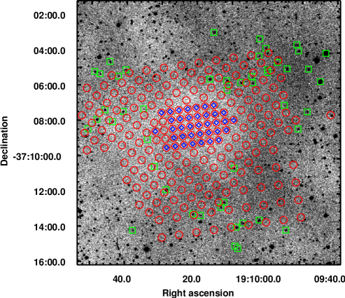
Figure 1: Data coverage of the sample over a negative infrared DSS image of SL42. The red field is the distribution of $\rm{C^{18}O}$ measurements, and the size of the circles corresponds to the HPBW of the antenna at 220 GHz (25^′′). The blue diamonds show the distribution of $\rm{N_{2}H^{+}}$ measurements. Locations where the observational noise exceeded the emission signals (i.e., S/N$<$1 or S$<$0) are not shown. The green squares indicate the locations of stars with good quality 2MASS $JHK$ photometry which met the condition $\hbox{$H-K$}>0.4$. The image center is located at R.A. 19^h10^m16$\fs$3, Decl. $-$37^∘08^′37^′′, J2000.0. The image is $\rm{15\hbox{${}^{\prime}$}\times 15\hbox{${}^{\prime}$}}$.

Radio data were collected using the 15 m Swedish ESO Submillimeter Telescope (SEST) in 2003 March. The molecular lines observed were $\rm{C^{18}O}$ $J=1-0$ (109.8 GHz), $\rm{C^{18}O}$ $J=2-1$ (219.6 GHz), and $\rm{N_{2}H^{+}}$ $J=1-0$ (93.2 GHz). A region of about $12\hbox{${}^{\prime}$}\times 8\hbox{${}^{\prime}$}$, centered on the ISOSS source 19102$-$3708 (R.A. 19^h10^m16$\fs$3, Decl. $-$37^∘08^′37^′′, J2000.0) was mapped in the two $\rm{C^{18}O}$ transitions simultaneously with the 3 and 1.3 mm superconductor-insulator-superconductor receivers, using a grid spacing of 40^′′. A region of $\sim$ 3^′ $\times$ 3^′ around the $\rm{C^{18}O}$ emission peak was thereafter mapped in $\rm{N_{2}H^{+}}$ $J=1-0$ and $\rm{C^{18}O}$ $J=2-1$ using a 20^′′ spacing. Figure 1 shows the coverage of the data field over a negative infrared Digitized Sky Survey (DSS) image of SL42.

All observations were performed in the frequency switching mode using an integration time of one minute per position. The two mixers used at the same time were connected to a 2000 channel acousto-optical spectrometer (AOS) which was split in two bands of 43 MHz each. The AOS channel width corresponds to 0.14 $\rm{km\leavevmode\nobreak\ s^{-1}}$ at 93 GHz, 0.12 $\rm{km\leavevmode\nobreak\ s^{-1}}$ at 110 GHz, and 0.06 $\rm{km\leavevmode\nobreak\ s^{-1}}$ at 220 GHz. The system temperatures were around 240, 260, and 450 K at 93, 110, and 220 GHz, respectively. The rms noise level attained was typically $\sim$ 0.1 K at 3 mm and $\sim$ 0.2 K at 1.3 mm.

The half-power beam width (HPBW) of the antenna was 47^′′ at 110 GHz and 25^′′ at 220 GHz. The pointing and focus were checked at 3$-$4 hr intervals toward circumstellar SiO maser line sources, and we estimate that the pointing accuracy was typically about 3^′′.

Calibration was done by the chopper wheel method. To convert the observed antenna temperatures ($T_{A}^{*}$) to the radiation temperatures ($T_{R}$) the former were divided by the assumed source-beam coupling efficiencies ($\eta_{C}$) for which we adopted the main beam efficiencies ($\eta_{MB}$) of the telescope interpolated to the frequencies used, i.e., 0.73, 0.71, and 0.61 at 93, 110, and 220 GHz, respectively.

2.2 SEST Data Reduction

The spectra were reduced using the Continuum and Line Analysis Single-dish Software (CLASS) program of the Grenoble Image and Line Data Analysis Software (GILDAS) package for the Institut de Radioastronomie Millim$\acute{e}$trique (IRAM). (See Figure 2 for example spectra.) The reduction involved the subtraction of the baseline using a polynomial fit and fitting Gaussian profiles to the detected lines to calculate the peak antenna temperatures ($T_{A}^{*}$), local standard of rest (LSR) velocities ($v_{\rm{LSR}}$), and the full-width half-max (FWHM) line widths ($\Delta v$). The intensities were converted to the main-beam brightness temperature scale by $T_{MB}=T_{A}^{*}/\eta_{MB}$, where $\eta_{MB}$ is the main-beam efficiency. Assuming uniform beam filling, $T_{MB}$ represents the brightness temperature $T_{B}$.

The $\rm{N_{2}H^{+}}$ $J=1-0$ lines contain seven hyperfine (hf) components. To fit the hf structure we used the frequencies and the relative line strengths given in Caselli et al. (1995). Besides $v_{\rm{LSR}}$ and $\Delta v$, the hf fit also gives the total optical depth ($\tau_{\rm{tot}}$) of the line which is the sum of peak optical thicknesses of the seven components. The fit can be used to calculate the optical depth profile ($\tau_{v}$) of the line (as a function of radial velocity $v$). The $\rm{C^{18}O}$ lines do not have hf structure, and the lines could be well fitted with a single Gaussian. The lines are likely to be optically thin in SL42, a relatively isolated, small cloud.

The $\rm{C^{18}O}$ and $\rm{N_{2}H^{+}}$ column densities were determined from the reduced spectra by assuming that the rotational levels are populated according to the local thermodynamic equilibrium (LTE). For $\rm{C^{18}O}$ it was furthermore assumed that the lines are optically thin.

When the excitation temperature ($T_{ex}$) and the integrated optical depth ($\int\tau_{v}dv$) of the observed transition $u\rightarrow l$ are known, the column density of the molecules in the upper level ($N_{u}$) can be calculated from the formula

$$N_{u}=\frac{8\pi}{\lambda^{3}}\frac{1}{A_{ul}}F(T_{ul},T_{ex})\int\tau_{v}dv,$$ (1)

where $A_{ul}$ is the Einstein coefficient for spontaneous emission, $\lambda=c/\nu_{ul}$ is the wavelength of the transition, $T_{ul}\equiv h\nu_{ul}/k_{B}$, and the function $F(T_{ul},T)$ is defined by

$$F(T_{ul},T)\equiv\frac{1}{e^{T_{ul}/T}-1}.$$ (2)

For an optically thin line, as in the case of $\rm{C^{18}O}$, the integral $\int\tau_{v}dv$ can be estimated from the integrated intensity using the antenna equation:

$$\int T_{B}(v)dv\approx T_{ul}[F(T_{ul},T_{ex})-F(T_{ul},T_{bg})]\int\tau_{v}dv.$$ (3)

For the derivation of the $\rm{C^{18}O}$ excitation temperature, the $\rm{C^{18}O}$ $J=2-1$ spectral map was convolved to the same angular resolution as the $J=1-0$ map, and the $T_{ex}$ was calculated from integrated intensity ratio of the two lines using the antenna equation.

The integrated $\tau$ of the $\rm{N_{2}H^{+}}$ line was obtained from hf fit results assuming a Gaussian profile:

$$\int\tau_{v}dv=\frac{\sqrt{\pi}}{2\sqrt{\ln{2}}}\Delta v\tau_{\rm{tot}}.$$ (4)

The $T_{ex}$ of $\rm{N_{2}H^{+}}$ was calculated by substituting the $T_{B}$ and $\tau$ values at the line peak into the antenna equation:

$$T_{B}(v)=T_{ul}[F(T_{ul},T_{ex})-F(T_{ul},T_{bg})](1-e^{-\tau_{v}}).$$ (5)

The total column densities ($N_{\rm{tot}}$) including all rotational levels were estimated according to the LTE assumption:

$$N_{\rm{tot}}=\frac{N_{u}}{g_{u}}e^{E_{u}/kT_{ex}}Z(T_{ex}),$$ (6)

where $Z(T_{ex})$ is the rotational partition function at the temperature $T_{ex}$, and $E_{u}$ is the energy of the level $u$ with respect to the rotational ground level.

2.3 Herschel Data

The $15\hbox{${}^{\prime}$}\times 15\hbox{${}^{\prime}$}$ Herschel maps of SL42 used in this study were extracted from the extensive mapping of the CrA region collected by the Spectral and Photometric Imaging Receiver (SPIRE) and Photodetector Array Camera and Spectrometer (PACS) instruments as part of the Herschel Gould Belt Survey (André et al. 2010; see also http://www.herschel.fr/cea/gouldbelt/en/). An overview of the Herschel Space Observatory is given in Pilbratt et al. (2010). The SPIRE and PACS instruments are described in Griffin et al. (2010) and Poglitsch et al. (2010), respectively.

The pipeline-reduced data from the SPIRE+PACS parallel mode survey of CrA are publicly available at the Herschel Science Archive. The original CrA maps cover a region of about $5\arcdeg\times 2\arcdeg$ at the wavelengths 500, 350, and 250 $\mu$m (SPIRE), and 160 and 70 $\mu$m (PACS). The FWHM values of the Gaussians fitted to the beam profiles are, in order of decreasing wavelength, 37^′′, 25^′′, 18^′′, 12$\hbox{${}^{\prime\prime}$}\times$16^′′, and 6$\hbox{${}^{\prime\prime}$}\times$12^′′, the PACS beams being clearly elongated in observations carried out in the parallel mode.

In order to calculate the distributions of the dust temperature ($T_{d}$) and the optical depth ($\tau_{\lambda}$) of the dust emission, the Herschel maps at 500, 350, 250, and 160 $\mu$m were first convolved with a Gaussian beam to a resolution of 40^′′ (FWHM), and the intensity distributions were fitted pixel by pixel with a modified blackbody function, $I_{\nu}\approx B_{\nu}(T_{d})\tau_{\nu}\propto B_{\nu}(T_{d})\nu^{\beta}$, which characterizes optically thin thermal dust emission at far-IR and submillimeter wavelengths. The observed values of $\beta$, the spectral index, are typically close to 2.0 (e.g., Boulanger et al. 1996; Schnee et al. 2010; Juvela et al. 2011), but higher values have been reported for cold regions (e.g., Dupac et al. 2003; Désert et al. 2008; Planck Collaboration et al. 2011). The recent study of the Taurus-Auriga molecular cloud found an average value of $\sim$ 1.8 but again significant anticorrelation between dust temperature and the spectral index. In our analysis we fixed the dust opacity spectral index to a constant value of $\beta=2.0$, which is used in several Herschel studies so the $T_{d}$ and $N(\hbox{$\rm{H_{2}}$})$ maps presented in this work are directly comparable with previous results. This is consistent with the Planck Early Cold Core (ECC) estimate for SL42, $\beta=2.4\pm 0.6$ (see Section 2.4), especially considering that the Planck value is the estimate for the cold dust component rather than for the total dust emission from this source. The pipeline-calibrated in-beam flux densities were color corrected to monochromatic flux densities at the standard wavelengths in the course of $T_{d}$ fitting using the adopted shape of the source spectrum (a modified blackbody spectrum with $\beta=2.0$) and the spectral response functions of SPIRE and PACS photometers for an extended source. In addition, the SPIRE pipeline in-beam flux densities were converted from point source calibration to extended source calibration before the temperature fitting and color correction.

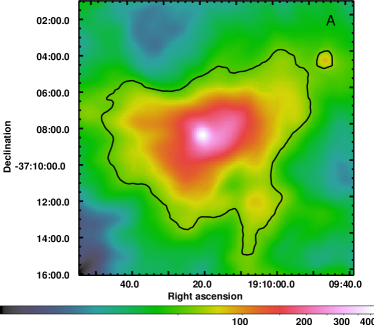
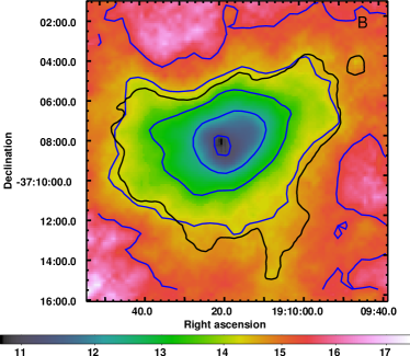
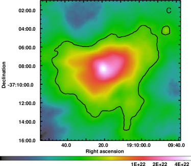
Figure 3: Colorbar units are MJy sr^-1, K, and cm^-2, respectively. (A) Herschel intensity map of thermal dust emission at the wavelength $\lambda=250\leavevmode\nobreak\ \hbox{$\mu$m}$ in a $15\hbox{${}^{\prime}$}\times 15\hbox{${}^{\prime}$}$ region around SL42. (B) Dust temperature map of the same region, created by fitting a modified blackbody function to the Herschel intensity maps at 500, 350, 250, and 160 $\mu$m (see Section 2.3). Blue contours range from 11 K at the center to 15 K in increments of 1 K. (C) $\rm{H_{2}}$ column density map determined from the far-infrared optical depth (see Equation (7)). The black contour shows where $N(\hbox{$\rm{H_{2}}$})=3.3\times 10^{21}\leavevmode\nobreak\ \rm{cm}^{-2}$.

The resulting intensity map ($I_{250\mu\rm{m}}$) at $\lambda$=250 $\mu$m and the $T_{d}$ map are shown in Figure 3. The optical depth map ($\tau_{250\mu\rm{m}}$), calculated from $\tau_{250\mu\rm{m}}=I_{250\mu\rm{m}}/B_{250\mu\rm{m}}(T_{d})$, is proportional to the molecular hydrogen column density ($N(\hbox{$\rm{H_{2}}$})$). The column density can be obtained from

$$N(\hbox{$\rm{H_{2}}$})=\frac{\tau_{250\mu\rm{m}}}{\kappa_{250\mu\rm{m}}{\bar{m}}_{\rm{H_{2}}}},$$ (7)

where $\kappa$ is the dust “opacity”, or absorption cross-section per unit mass of gas, and ${\bar{m}}_{\rm{H_{2}}}$ ($=2.8$ amu $=4.65\times 10^{-24}$ g) is the average mass of gas per $H_{2}$ molecule (assuming 10% He). The $\rm{H_{2}}$ column density errors were estimated by a Monte Carlo method using the $1\sigma$ error maps provided for the three SPIRE bands and a 7% uncertainty of the absolute calibration for all four bands according to the information given in SPIRE and PACS manuals. Different realizations of the $N(\hbox{$\rm{H_{2}}$})$ map were calculated by combining the four intensity maps with the corresponding error maps, assuming that the error in each pixel is normally distributed. The $N(\hbox{$\rm{H_{2}}$})$ error in each pixel was obtained from the standard deviation of one thousand realizations. For the dust opacity at 250 $\mu$m, we used the value $\kappa_{250\mu\rm{m}}^{\rm g}=0.085\leavevmode\nobreak\ {\rm cm^{2}\leavevmode\nobreak\ g^{-1}}$ which is a factor of 1.17 lower than the value $\kappa_{250\mu\rm{m}}^{\rm g}=0.1\leavevmode\nobreak\ {\rm cm^{2}\leavevmode\nobreak\ g^{-1}}$ consistent with the parameter $C_{250}\leavevmode\nobreak\ (=1/\kappa_{250\mu\rm{m}})$ given in Table 1 of Hildebrand (1983). This choice was motivated by the comparison between $\rm{H_{2}}$ column densities from Herschel and visual extinctions from 2MASS as described in Section 3.2.

2.4 ISOPHOT and Planck Observations of Infrared Continuum Emission

The Infrared Space Observatory photo-polarimeter (ISOPHOT) Serendipity Survey (ISOSS) recorded the 170 $\mu$m sky brightness when the satellite was slewing between two pointed observations. SL42 is one of the “cold cores” (Tóth et al., 2000) detected in this survey. The dust temperature calculated by correlating the ISOPHOT 170 $\mu$m and Infrared Astronomical Satellite (IRAS)/IRAS Sky Survey Atlas (ISSA) 100 $\mu$m intensities is $T_{d}=11.1^{+1.8}_{-0.8}$ K. A detailed description of the method can be found in Hotzel et al. (2001). The ISOPHOT detector had four pixels with slightly different tracks. The width of the slew was about $3^{\prime}$, and the effective angular resolution in the scan direction was $2\farcm 2$. The surface brightness distribution recorded by the two pixels which passed near the cloud center shows a Gaussian bump. It has an FWHM of $5\farcm 7$ and a maximum intensity of 52 MJy $\rm{sr}^{-1}$. Assuming spherical symmetry, the total 170 $\mu$m flux density of the core is 162 Jy. It sits on top of a 15 MJy $\rm{sr}^{-1}$ pedestal, which is likely to correspond to the low-density envelope around the core. Its position was used as the origin position for the SEST observations.

SL42 can be found in the Planck Early Release Compact Source Catalogue (ERCSC) as the object PLCKECC G000.37$-$19.51. The core is detected at the Planck frequencies from 100 to 857 GHz ($\lambda=3.0-0.35$ mm). The coordinates of the 857 GHz maximum (PLCKERC857 G000.36$-$19.49) are at R.A. and Decl. offsets $(51\hbox{${}^{\prime\prime}$},-9\hbox{${}^{\prime\prime}$})$ from the SEST origin. The dust temperature and the emissivity index in the cold core are $T_{d}=10.2\pm 0.6$ K and $\beta=2.4\pm 0.6$, respectively. These are calculated from the 857, 545, and 353 GHz fluxes, after the subtraction of the warm component (see the Explanatory Supplement). The ERCSC gives furthermore a total flux density $S_{857\rm{GHz}}=271\pm 9$ Jy and an angular size of $6\farcm 9\times 6\farcm 1$ (FWHM) for the core. The Planck beam (FWHM) is $5\farcm 1\times 3\farcm 9$ at 857 GHz. The beam size is similar at other submillimeter wavelengths.

3 Analysis

3.1 $\rm{C^{18}O}$ and $\rm{N_{2}H^{+}}$ Maps, Line Characteristics, and Column Densities

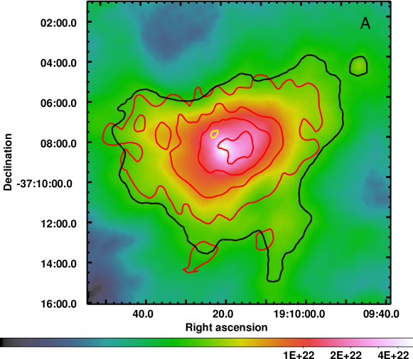
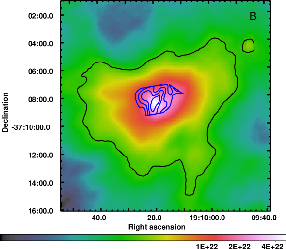
Figure 4: Contour maps of (A) $\rm{C^{18}O}$ and (B) $\rm{N_{2}H^{+}}$ superimposed on the $\rm{H_{2}}$ column density map of SL42. The contours for $\rm{C^{18}O}$ (red) range from 1 to 4 $\rm{(10^{15}\leavevmode\nobreak\ cm^{-2})}$ in increments of 1; yellow indicates a depression contour. The contours for $\rm{N_{2}H^{+}}$ (blue) range from 2 to 11 $\rm{(10^{12}\leavevmode\nobreak\ cm^{-2})}$ in increments of 3. The maximum $\rm{C^{18}O}$ detection is located at (0^′′, 0^′′), and the maximum $\rm{N_{2}H^{+}}$ detection is located at (34^′′, 25^′′) giving a spatial offset of $\sim$ 42^′′ ($\sim$ 5500 AU at a distance of 130 pc). The black contour shows where $N\rm{(\hbox{$\rm{H_{2}}$})=3.3\times 10^{21}\leavevmode\nobreak\ cm^{-2}}$. The colorbars are in units of cm^-2.

Figure 4 shows the column density maps of the $\rm{C^{18}O}$ $J=2-1$ and $\rm{N_{2}H^{+}}$ $J=1-0$ lines. A maximum $\rm{C^{18}O}$ detection of 4.53 $\pm$ 0.09 ($\rm{10^{15}\ cm^{-2}}$) occurs at positional offsets of $(0\hbox{${}^{\prime\prime}$},0\hbox{${}^{\prime\prime}$})$, and a maximum $\rm{N_{2}H^{+}}$ detection of 13.40 $\pm$ 1.60 ($\rm{10^{12}\ cm^{-2}}$) occurs at positional offsets of $(34\hbox{${}^{\prime\prime}$},25\hbox{${}^{\prime\prime}$})$. The $\rm{C^{18}O}$ $J=2-1$ and $\rm{N_{2}H^{+}}$ $J=1-0$ line parameters and total $N(\hbox{$\rm{C^{18}O}$})$ and $N(\hbox{$\rm{N_{2}H^{+}}$})$ toward both the mentioned maxima and the second brightest positions in each molecule are listed in Table 1. The spectra from these four positions are shown in Figure 2.

3.2 Visual Extinction ($A_{V}$)

Dust extincts light from background sources via absorption and scattering to make them appear redder and dimmer. We used two methods in order to estimate the amount of visual extinction, and thereby dust, in SL42. First, visual extinctions ($A_{V}$) were determined using Two Micron All Sky Survey (2MASS) $JHK$ photometry as described in Shenoy et al. (2008) for field stars toward SL42 (marked in green in Figure 1).

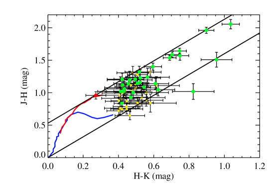
Figure 5: Color-color diagram of all reddened ($\hbox{$H-K$}>0.4$) field stars behind SL42 (equivalent to the green squares in Figure 1.) Green circles denote stars within the SEST data field, while yellow circles denote stars beyond the SEST field. H$\alpha$ 16 is shown as a red point below the $H-K$ cutoff. The reddening slope for SL42 is 1.6. Red and blue mark the intrinsic color lines for giants and dwarfs, respectively.

Figure 5 shows the color-color diagram for all of the field stars employed in this $A_{V}$ survey. We included only those stars from the catalog without flags indicating contamination or poor photometric quality of the observations. To remove unreddened or anomalous stars from the sample, the following color constraints were applied:

$$\mathrm{1.6(\hbox{$H-K$})+0.0<(\hbox{$J-H$})<1.6(\hbox{$H-K$})+0.53}$$ (8)

$$\mathrm{0.4<(\hbox{$H-K$})}.$$ (9)

The value of the reddening vector for the entire CrA cloud is 1.6, but the slope in the $J-H$ versus $H-K$ diagram does not change when only the SL42 region is considered. Stars outside of the parallel lines in Figure 5 were excluded since they could not be dereddened to the intrinsic color lines.

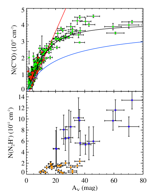
Figure 6: Top: $\rm{C^{18}O}$ column density as a function of extinction. Red points: Interpolated $N(\hbox{$\rm{C^{18}O}$})$ and field star extinctions from 2MASS $JHK$ photometry. Green points: SEST $N(\hbox{$\rm{C^{18}O}$})$ and extinctions from Herschel maps using $N(\hbox{$\rm{H_{2}}$})/\hbox{$A_{V}$}=9.4\times 10^{20}\rm{cm^{-2}\leavevmode\nobreak\ mag^{-1}}$ from Bohlin et al. (1978). Blue line: sigmoidal fit to data from the Taurus cloud (see Whittet et al. 2010 for details). Red line: average fit based on observations of molecular clouds with low depletion ($N=2.0\times 10^{14}\rm{(\hbox{$A_{V}$}\ -2.0)\leavevmode\nobreak\ cm^{-2}}$) (Kainulainen et al., 2006). Black line: sigmoidal fit to SL42 data ($N=4.07953+(0.14037-4.07953)/(1+(\hbox{$A_{V}$}/11.27966)^{1.55722})\leavevmode\nobreak\ \rm{cm^{-2}}$). Bottom: SEST $N(\hbox{$\rm{N_{2}H^{+}}$})$ and extinctions from Herschel maps. Blue points: $N(\hbox{$\rm{N_{2}H^{+}}$})$ found by fitting the hyperfine structure of the spectral feature. Orange points: $N(\hbox{$\rm{N_{2}H^{+}}$})$ found assuming optically thin conditions.

It should be noted that the visual extinctions calculated from the 2MASS color-color diagram are conservative estimates. They were calculated using the minimum possible color excesses ($E(J-K)$) necessary to place the reddened field stars on the intrinsic color lines. Most of the reddening vectors of the field stars in our sample cross the intrinsic color lines in two places, once in a region of late spectral type and once in a region of early spectral type. It is likely that most of our field stars are of late spectral type, so the minimum extinction values we have assumed are correct. Even if this is not the case for all of the field stars, the maximum extinction values are higher at most by a factor of two, and accounting for a few early type stars should not significantly change the trend seen in Figure 6, detailed in Section 5.

Figure 5 presents no clear evidence for previously unknown YSOs in SL42. This is consistent with the Herschel data, which confirm that SL42 is a starless core because the dust temperature decreases toward the center of the cloud. H$\alpha$ 16 appears in Figure 5 as the red point below our $H-K$ color cutoff. Wilking et al. (1992) classify H$\alpha$ 16 as a class II YSO by its spectral energy distribution (SED).

The 2MASS method for estimating extinction is considered reliable because it measures its effects directly without making assumptions about the emissive properties of the intervening dust. However, this method is only useful in the outer regions of SL42 because the opacity in the core is so high that field stars become undetectable. In order to sample the cloud’s extinction more completely, we used the canonical relationship $N(\hbox{$\rm{H_{2}}$})/\hbox{$A_{V}$}=9.4\times 10^{20}$ cm^-2 mag^-1 (Bohlin et al., 1978; Martin et al., 2012) as a second method to obtain dust extinction values using Herschel data. The calculation of $N(\hbox{$\rm{H_{2}}$})$ from the Herschel intensity maps of SL42 depends inversely on the assumed dust opacity (see Equation (7)); therefore, it is important that the correct value of kappa is chosen. The 2MASS photometry provides an independent measurement of extinction at the edge of the cloud, so we adjusted $\kappa_{250\mu\rm{m}}^{\rm g}$ such that $N(\hbox{$\rm{H_{2}}$})$ estimates from Herschel converted to $A_{V}$ overlap the 2MASS data at low extinctions. This scaling gives a value of $\kappa_{250\mu\rm{m}}^{\rm g}=0.085\leavevmode\nobreak\ {\rm cm^{2}\leavevmode\nobreak\ g^{-1}}$.

3.3 Mass and Dynamical State

The $\rm{H_{2}}$ column density map created from Herschel data as described in Section 2.3 can be used to estimate the cloud mass. By choosing the region above $N({\hbox{$\rm{H_{2}}$}})=3.3\times 10^{21}$ cm^-2 (corresponding to $\hbox{$A_{V}$}=3.5$ when the relationship $N(\hbox{$\rm{H_{2}}$})/\hbox{$A_{V}$}=9.4\times 10^{20}$ cm^-2 mag^-1 of Bohlin et al. (1978) is adopted) we obtain a mass of $21\leavevmode\nobreak\ M_{\odot}$ at the assumed distance of 130 pc.

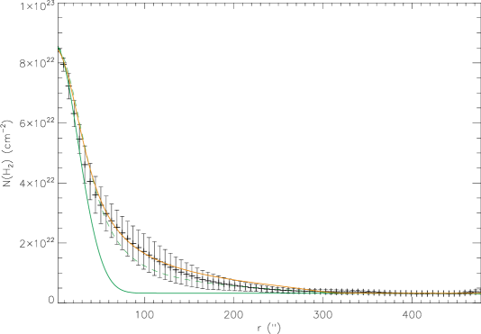
Figure 7: Azimuthally averaged $\rm{H_{2}}$ column density distribution of SL42 as a function of radial distance in arcseconds from the maximum (crosses), which occurs at R.A. 19^h10^m20$\fs$2, Decl. $-$37^∘08^′26^′′, J2000.0, or offsets from the SEST origin of (46^′′, 11^′′). The solid orange curve shows the $\rm{H_{2}}$ column density calculated from a spherically symmetric density profile following the function $n(r)=n_{0}/(1+(r/r_{0})^{2})$, where $n_{0}=1.2\times 10^{6}$ cm^-3, and $r_{0}=15\hbox{${}^{\prime\prime}$}$. The solid green curve represents a critically stable Bonnor-Ebert sphere ($\xi_{\rm out}=6.45$) with the maximum column density agreeing with the observed one. The observed distribution can be fitted fairly well also with a highly super-critical ($\xi_{\rm out}\sim 25$) Bonnor-Ebert sphere (dashed green curve).

The derivation of the gravitational potential energy requires an assumption about the density distribution in the cloud. The $\rm{H_{2}}$ column density map has a sharp maximum at the offsets (46^′′, 11^′′), R.A. 19^h10^m20$\fs$2, Decl. $-$37^∘08^′26^′′, J2000.0, from the origin of our molecular line maps. We calculated the azimuthally averaged $\rm{H_{2}}$ column density profile using this position as the cloud center. The result of the calculation is shown in Figure 7.

We also made an attempt to fit the azimuthally averaged column density distribution with a “Plummer-type” (Whitworth & Ward-Thompson, 2001; Plummer, 1911) outwardly decreasing number density profile using the following functional form:

$$n(r)=\frac{n_{0}}{\left(1+\frac{r^{2}}{r_{0}^{2}}\right)^{\eta/2}}\leavevmode\nobreak\ \mbox{when}\leavevmode\nobreak\ r\leq R_{\rm{out}},$$ (10)

where $n(r)$ is the number density of $\rm{H_{2}}$ as a function of radius $r$, $n_{0}$ is the gas number in the cloud center, $r_{0}$ is the “flat radius” representing the radial distance where the density increase toward the center levels off, and $R_{\rm{out}}$ is the radius inside which this density profile is supposed to be valid. We assumed that the cloud envelope outside this radius has a constant $\rm{H_{2}}$ column density that forms a pedestal on top of which we see the column density enhancement owing to the cloud core.

The best fit to the data is obtained with the following parameter values: $\eta=2.0$, $n_{0}=1.2\times 10^{6}$ cm^-3, $r_{0}=15\farcs 0$, and $R_{\rm{out}}=300\hbox{${}^{\prime\prime}$}$. The exponent value $\eta=2$ means that the density distribution approaches $n(r)\propto r^{-2}$ for $r\gg r_{0}$. The average column density far from the cloud center, $N(\hbox{$\rm{H_{2}}$})=3.3\times 10^{21}$ cm^-2 (corresponding to $\hbox{$A_{V}$}=3.5$) is used as the “pedestal” added to $N(\hbox{$\rm{H_{2}}$})$ obtained from the density model. The predicted column density profile (convolved with a Gaussian to 40^′′ resolution to allow comparison with the observed one) is indicated as a dashed line in Figure 7. The core mass calculated from the adopted $\rm{H_{2}}$ density profile up to $r=R_{\rm{out}}$ is $M_{\rm{core}}=16\leavevmode\nobreak\ M_{\odot}$. The $5\leavevmode\nobreak\ M_{\odot}$ difference between the model mass and the cloud mass from the $N(\hbox{$\rm{H_{2}}$})$ map is accounted for by the “pedestal” with $N(\hbox{$\rm{H_{2}}$})=3.3\times 10^{21}$ cm^-2.

The agreement between the observed (averaged) and predicted $N(\hbox{$\rm{H_{2}}$})$ distributions is reasonably good, and we used the model density distribution to calculate the gravitational potential energy of the core ($E_{\rm{grav}}$) from the integral

$$E_{\rm{grav}}=-16\pi^{2}G{{\bar{m}}_{\rm{H_{2}}}}^{2}\int_{0}^{R_{\rm{out}}}rn(r)dr\int_{0}^{r}y^{2}n(y)dy=-1.0\times 10^{37}\leavevmode\nobreak\ \rm{J},$$ (11)

where $G$ is the gravitational constant and ${\bar{m}}_{\rm{H_{2}}}$ ($=2.8$ amu $=4.65\times 10^{-24}$ g) is the average mass of gas per $H_{2}$ molecule (assuming 10% He, $n(r)=n_{\rm{H_{2}}}(r)$). In the kinetic energy estimate we assumed the cloud gas is isothermal with $T_{\rm{kin}}=10$ K and has a constant non-thermal velocity dispersion, $\sigma_{\rm{N.T.}}=260$ m s^-1. The latter value is calculated from the $\rm{C^{18}O}$ spectra in the core region. Using these values we obtain

$$E_{\rm{kin}}=\frac{3}{2}M_{\rm{core}}[c_{s}^{2}+\sigma_{\rm{N.T.}}^{2}]=5.0\times 10^{36}\leavevmode\nobreak\ \rm{J},$$ (12)

where

$$c_{s}\equiv\sqrt{k_{B}T_{\rm{kin}}/{\bar{m}}}$$ (13)

is the isothermal sound speed, ${\bar{m}}=2.33$ amu is the average particle mass of the gas. We see that according to the estimates above, the core satisfies the equation, $E_{\rm{grav}}+2E_{\rm{kin}}=0$, which in the absence of external pressure would indicate virial equilibrium. However, our cloud model also includes a low density envelope which should be exerting pressure on the core, so it seems the cloud is lacking sufficient thermal and/or turbulent support against collapse.

The estimation of the kinetic and potential energies involves some uncertainties. The gas kinetic temperature is not directly measured, but we use the average dust temperature. Also, the $\rm{H_{2}}$ column densities from thermal dust emission are calculated using color temperatures and a constant dust opacity. The systematic errors related to these approximations are difficult to estimate. The color temperature is larger than the true temperature in the core center (Nielbock et al., 2012; Juvela & Ysard, 2012; Malinen et al., 2011), and using the former temperatures we probably underestimate the $\rm{H_{2}}$ column densities and the mass. On the other hand, varying the temperature by 1 K and the velocity dispersion by one spectrometer channel changes the estimate of kinetic energy by 30 percent. Nevertheless, it is remarkable that our best effort estimates suggest a balance $2E_{\rm{kin}}/|E_{\rm{grav}}|\sim 1$, showing that the core is gravitationally bound (McKee & Ostriker, 2007).

4 Modeling

We have attempted to reproduce the observed $\rm{C^{18}O}$ and $\rm{N_{2}H^{+}}$ line profiles (Figure 2) and the associated column densities (Table 1) by calculating simulated radial abundance profiles for $\rm{C^{18}O}$ and $\rm{N_{2}H^{+}}$ using a chemical model and by using the abundance profiles as input for a radiative transfer program. We now discuss the modeling process and present the results.

4.1 Chemical Modeling

To simulate chemical evolution in the core, we divided the Plummer sphere discussed in Section 3.3 into 40 concentric shells. Chemical evolution was then calculated separately in each shell, yielding radial abundance profiles as a function of time — the chemical model (and the general modeling procedure) used here is the same as the one discussed in detail in Sipilä (2012). The gas phase chemical reactions are adopted from the OSU reaction file osu_03_2008. The initial gas phase abundances and the surface reaction set (i.e., activation energies for select reactions) are adopted from Semenov et al. (2010). For the chemical calculations, the visual extinction was calculated from the density profile as a function of core radius assuming $\hbox{$A_{V}$}=3$ at the edge of the model core. In the calculations, it is assumed that all grains are 0.1 $\mu$m in radius and that the cosmic ionization rate is $\zeta=1.3\times 10^{-17}\leavevmode\nobreak\ \rm{s}^{-1}$.

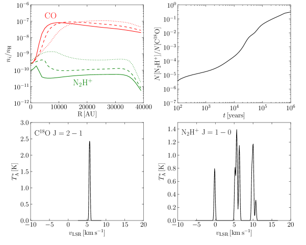
Figure 8: Upper left: $\rm{C^{18}O}$ (red) and $\rm{N_{2}H^{+}}$ (green) radial abundances with respect to total hydrogen density $n_{\rm{H}}$ in the chemical model at $t=4\times 10^{4}$ years (solid lines), $t=8\times 10^{4}$ years (dashed lines) and $t=2\times 10^{5}$ years (dotted lines). Upper right: the ratio of $\rm{N_{2}H^{+}}$ and $\rm{C^{18}O}$ column densities through the center of the core model as a function of time. Lower left: the simulated $\rm{C^{18}O}$ $J=2-1$ line emission profile at $t=4.5\times 10^{4}$ years in the antenna temperature scale. Lower right: the simulated $\rm{N_{2}H^{+}}$ $J=1-0$ line emission profile at $t=4.5\times 10^{4}$ years in the antenna temperature scale.

The upper left panel in Figure 8 shows the radial abundance profiles of $\rm{C^{18}O}$ and $\rm{N_{2}H^{+}}$ (with respect to total hydrogen density $n_{\rm{H}}$ at three different time steps). Evidently the two species evolve very differently. $\rm{C^{18}O}$ is strongly depleted at the core center at later times but retains a fairly constant abundance at the core edge as the core grows older. $\rm{N_{2}H^{+}}$ on the other hand increases greatly in abundance throughout the core as time progresses. The upper right panel of Figure 8 shows the ratio of the column densities of $\rm{N_{2}H^{+}}$ and $\rm{C^{18}O}$ through the center of the model core as a function of time; the growth of the $\rm{N_{2}H^{+}}$ abundance with respect to the $\rm{C^{18}O}$ abundance as the core grows older is especially prominent here.

The $\rm{C^{18}O}$ column density map of the spherically symmetric model cloud has a ring-like maximum with a radius of $\sim$ 40^′′ (5000 AU). In the convolved (40^′′ resolution) image, the slight depression at the core center has about 10% lower column density than the annular maximum. The corresponding $\rm{N_{2}H^{+}}$ map shows a sharp peak toward the core center. The widths (FWHM) of the $\rm{C^{18}O}$ and $\rm{N_{2}H^{+}}$ distributions are 200^′′ and 60^′′, respectively. The model can thus qualitatively explain the different extents of the $\rm{C^{18}O}$ and $\rm{N_{2}H^{+}}$ emissions and the fact that these molecules can peak at different locations.

The observed $\rm{C^{18}O}$ maximum does not lie, however, symmetrically around the $N(\hbox{$\rm{H_{2}}$})$ maximum but on its northwestern side. Possibly this can be understood in terms of the asymmetric $\rm{H_{2}}$ column density distribution which has a shoulder on the side where $\rm{C^{18}O}$ peaks, and decreases more rapidly in other directions (see Figure 4(A)).

4.2 Spectral Line Modeling

We attempted to reproduce the observed spectra toward the $\rm{N_{2}H^{+}}$ peak by calculating simulated $\rm{N_{2}H^{+}}$ $J=1-0$ and $\rm{C^{18}O}$ $J=2-1$ line emission profiles with a Monte Carlo radiative transfer program (Juvela, 1997), using the chemical modeling results as input. The simulated spectra are highly dependent on the radial abundances and hence on the column densities of $\rm{N_{2}H^{+}}$ and $\rm{C^{18}O}$, which are both variable functions of time (Figure 8).

The column density ratio of $\rm{C^{18}O}$ and $\rm{N_{2}H^{+}}$ toward the (34^′′, 25^′′) position (cf. Table 1) corresponds roughly to $t\sim 4-5\times 10^{4}$ years in the model. The lower left and lower right panels of Figure 8 show the simulated $\rm{C^{18}O}$ $J=2-1$ and $\rm{N_{2}H^{+}}$ $J=1-0$ line profiles, respectively, at $t\sim 4.5\times 10^{4}$ years. The observed peak intensities (cf. Table 1) are reproduced rather well by the model at this time step. However, the optical depths of the model lines are much smaller than the observed thicknesses. This is tied to the column densities predicted by the model; while the $\rm{N_{2}H^{+}}$ and $\rm{C^{18}O}$ column density ratio in the model corresponds to the observed ratio at $t\sim 4.5\times 10^{4}$ years, the actual column densities for both species are at this time clearly smaller than observed. This suggests that the observed column densities correspond to a later stage in the model.

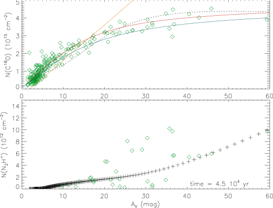
Figure 9: Chemical modeling fits to SL42 observations. Green diamonds correspond to observed data. The dashed black line (top panel) and black crosses (bottom panel) show the best fits of the Sipilä (2012) model, while the red line shows the best fit from the Keto & Caselli (2008) model. The sigmoidal function fitted to the $\rm{C^{18}O}$ data is shown in blue, and the empirical fit to undepleted clouds (Kainulainen et al., 2006) is in orange.

To compare the observed and modeled column densities across the cloud we have plotted these in Figure 9 as functions of the visual extinction $A_{V}$, calculated from Herschel (using $N(\hbox{$\rm{H_{2}}$})/\hbox{$A_{V}$}=9.4\times 10^{20}\leavevmode\nobreak\ \rm{cm}^{-2}\leavevmode\nobreak\ \rm{mag}^{-1}$). The model distribution corresponds to $t\sim 4.5\times 10^{4}$ years. It is evident that the observed $\rm{C^{18}O}$ column density rises much more steeply with increasing $A_{V}$ than predicted by the model. The model either undervalues the CO production through gas-phase reactions and desorption or uses too high estimates for the CO destruction rates (through photodissociation and accretion) in low-density gas. Alternatively, the discrepancy is caused by the fact that the static model adopted here does not take account of the increase of the density in case the core is contracting. We return to this issue in Section 5.3

5 Discussion

5.1 CO Depletion

CO is expected to become depleted from the gas phase by adsorption onto grains on timescales less than the expected lifetimes of dense cores (e.g., Whittet et al. 2010 and references therein). In a detailed study of the Taurus dark-cloud complex, Whittet et al. (2010) compare gas phase and solid phase CO in lines of sight toward background field stars with known extinction values from 2MASS data. They find that (1) the total CO (gas + solid) column density agrees well with the general relation $N=2.0\times 10^{14}(\hbox{$A_{V}$}-2.0)\leavevmode\nobreak\ {\rm cm}^{-2}$ proposed by Kainulainen et al. (2006); and (2) depletion begins to become significant at extinctions $\hbox{$A_{V}$}\gtrsim 5-10$ in the Taurus cloud.

The plot of $N(\hbox{$\rm{C^{18}O}$})$ versus $A_{V}$ based on our observations and extinction estimates data from 2MASS and Herschel is shown in Figure 6. The straight line is the linear relation from Kainulainen et al. (2006), and the clear divergence of the data from this line at high extinctions ($\hbox{$A_{V}$}\gtrsim 15$) is most likely caused by depletion. No data on ice-phase abundances are available that would allow us to directly quantify the uptake of CO into grain mantles in SL42, but we note that the form of the variation of $N(\hbox{$\rm{C^{18}O}$})$ with $A_{V}$ in Figure 6 is qualitatively very similar to that found by Whittet et al. (2010) for Taurus. This variation can be described by a sigmoidal function of the form $y=a_{2}+(a_{1}-a_{2})/(1+(x/x_{0})^{p})$. A fit of this form to our data for SL42 is shown in Figure 6 and compared with the corresponding curve for Taurus from Whittet et al. (2010). We conclude that the $N(\hbox{$\rm{C^{18}O}$})$ versus $A_{V}$ relation in SL42 follows the same general empirical law as that found for Taurus, but with lower levels of depletion.

As previously mentioned, the Herschel $A_{V}$ data in Figure 6 were scaled in order to match 2MASS data at low extinctions. The scaling was uniform and made under the assumption that the dust opacity ($\kappa_{250\mu\rm{m}}$) remains constant throughout the cloud. Martin et al. (2012) found that this assumption is not necessarily true; in the dense molecular interstellar medium of the galactic plane, the dust opacity increases with decreasing temperature. Because our dust temperature maps are averaged along the line of sight, it is not possible to correct for the likely increasing dust opacity at the core of SL42. However, the dust opacity should vary at most by a factor of $2-3$ times from edge to core of SL42, and this would effectively compress Figure 6 along the $x$-axis, only at the highest extinctions. The general conclusion of CO depletion at the core of SL42 would be unaffected.

The offsets in peak $\rm{C^{18}O}$ and $\rm{N_{2}H^{+}}$ concentrations provide supporting evidence for CO depletion in the core of SL42. Offsets between $\rm{C^{18}O}$ and $\rm{N_{2}H^{+}}$ are seen in many other starless cores, e.g., L1498, L1495, L1400K, L1517B, L1544 (Tafalla et al., 2002), and Barnard 68 (Lada et al., 2003). The differentiation of $\rm{N_{2}H^{+}}$ and CO originates from the main production pathway of $\rm{N_{2}H^{+}}$ in the reaction between ${\rm N_{2}}$ and ${\rm H_{3}^{+}}$. The ${\rm N_{2}}$ molecule is formed from relatively slow neutral-neutral reactions, and its abundance builds up later than that of CO. On the other hand, the ${\rm H_{3}^{+}}$ ion increases strongly only after the depletion of CO in the densest parts of molecular clouds. The different behaviors of C-bearing and N-bearing species have been discussed, e.g., by Flower et al. (2005) and by Fontani et al. (2012), see their Appendix A. At very late stages of chemical evolution $\rm{N_{2}H^{+}}$ is also likely to become depleted, but previous observations suggest that even then the $\rm{N_{2}H^{+}}$$/$CO abundance ratio remains high. One possible explanation suggested by Flower et al. (2005) is that a low sticking coefficient of atomic N could contribute to the availability of ${\rm N_{2}}$ also in highly depleted regions.

5.2 Dynamics

The Plummer-like density profile with three parameters, $n_{0}$ (the central density), $r_{0}$ (the characteristic radius of the inner region with a flat density distribution), and $\eta$ (describing the density power-law far from the center) has been used in several previous studies for fitting the observed column density profiles of prestellar cores or starless filaments (Whitworth & Ward-Thompson, 2001; Tafalla et al., 2002). Dust continuum maps have often suggested very steep ($\eta\geq 4$) density gradients near the edges of prestellar cores (Whitworth & Ward-Thompson, 2001), but in the case of SL42 the azimuthally averaged column density profile can be fit with $\eta=2$ up to a radial distance where the core is melted into the envelope of low-column density gas. Tafalla et al. (2002) found similar outer profiles as in SL42 for the prestellar cores L1495 and L1400K.

The average density profile obtained for SL42, $n(r)=n_{0}/(1+(r/r_{0})^{2})$, can also be used to approximate a Bonnor-Ebert sphere (BES), which is a pressure-bound, isothermal, hydrostatic sphere. As evident from Figure 7, the structure of SL42 differs, however, clearly from a critical BES which has been frequently used to describe globules and dense cores (e.g., Alves et al. 2001). The distribution, with a small flat radius $r_{0}$ compared to the outer radius of the core corresponds to a highly super-critical BES with $\xi_{\rm out}\sim 25$ where the balance between forces is unstable against any increase of the outside pressure (dashed green line in Figure 7). The overall agreement is, however, better with the adopted Plummer-like function with $n(r)\sim r^{-2}$ at large radii.

Clear deviations from the critical BES structure have been previously seen in clouds with regular shapes other than SL42. Kandori et al. (2005) found in their NIR study of Bok globules that while several starless globules can be approximated by nearly critical BESs with $\xi_{\rm out}=6.5\pm 2$, the column density profiles of star forming globules resemble those for super-critical BESs. The largest value of $\xi_{\rm out}$ was found for the core L694-2 with in-fall features in molecular line spectra. The hydrodynamical models of Kandori et al. (2005) are consistent with these observations: collapsing cores mimic super-critical BESs with $\xi_{\rm out}$ increasing with time.

A density distribution approaching the power-law $n(r)\propto r^{-2}$ at large values of $r$ was found in the early numerical simulations of the collapse of an isothermal sphere by Bodenheimer & Sweigart (1968) and Larson (1969), and the existence of a self-similar solution with this form was shown by Penston (1969) by analytic methods. This motivated Keto & Caselli (2010) to describe the collapse of a prestellar core by a sequence of BESs where the central density increases and the flat radius decreases while the outer radius is constant and the density profile in the outer parts keeps its scaling as $r^{-2}$ (see their Figure 1). The density distribution approaches that of a singular isothermal sphere ($n(r)\propto r^{-2}$ throughout) which is the initial configuration in the inside-out collapse model of Shu (1977).

Keto & Caselli (2010) predict the flat radius $r_{0}$ to be equal to the product of the sound speed and the free-fall time in the core center (see their Equation (2)). Allowing for turbulent velocity dispersion we may write a slightly modified formula for $r_{0}$:

$$r_{0}=\sqrt{\frac{3\pi(c_{s}^{2}+\sigma_{\rm{N.T.}}^{2})}{32G\rho_{0}}},$$ (14)

where $\rho_{0}$ is the central density. Substituting the adopted values of the parameters, $T_{\rm{kin}}=10$ K, $\sigma_{\rm{N.T.}}=260$ m s^-1, $n_{0}=1.2\times 10^{6}$ cm^-3, we get for the expected flat radius $r_{0}=1900$ AU or 15^′′, i.e., the same value as determined from the observations.

The calculated density profile and the agreement between the flat radius with the theoretical prediction suggest that SL42 is indeed contracting. According to the model of Keto & Caselli (2010) the contraction speed is highest around the flat radius (15^′′ in our case) and clearly subsonic at this stage of the evolution. The detection of infall is not possible with the resolution and sensitivity of the present data.

5.3 Modeling

Our pseudo-time dependent chemistry model discussed in Sections 4.1 and 4.2 failed to reproduce the $\rm{C^{18}O}$ column densities in the outer parts of SL42. Judging from the deduced density profile, the cloud is evolving dynamically, and probably the main difficulty here is to find realistic initial conditions for the chemistry taking the earlier history of the cloud into account. In their genuinely time-dependent model for a contracting core, Keto & Caselli (2010) found that CO reaches its equilibrium abundance in a short time compared with the dynamical timescale. It seems therefore justified to examine if a steady-state model can explain the observed $\rm{C^{18}O}$ column density profile.

Assuming a steady state, the fractional $\rm{C^{18}O}$ abundance can be described by a simple function of the gas density. The accretion and desorption rates (${\rm cm^{-3}\leavevmode\nobreak\ s^{-1}}$) in an isothermal cloud can be written as $An(\hbox{$\rm{H_{2}}$})n(\hbox{$\rm{C^{18}O}$},{\rm gas})=An(\hbox{$\rm{H_{2}}$})^{2}X(\hbox{$\rm{C^{18}O}$},{\rm gas})$ and $Bn(\hbox{$\rm{C^{18}O}$},{\rm dust})=Bn(\hbox{$\rm{H_{2}}$})X(\hbox{$\rm{C^{18}O}$},{\rm dust})$, respectively. The adsorption coefficient $A$ and the desorption coefficient $B$ depend on the dust properties, temperature, and the flux of heating particles (e.g., Leger et al. 1985; Hasegawa & Herbst 1993; Caselli et al. 2002; Hotzel et al. 2002; Keto & Caselli 2008, 2010). The coefficients $A$ and $B$ have the following relationships with the desorption and depletion timescales, $\tau_{\rm ON}$ and $\tau_{\rm OFF}$, defined by Keto & Caselli (2008): $An(\hbox{$\rm{H_{2}}$})=1/\tau_{\rm ON}$, $B=1/\tau_{\rm OFF}$. The definitions of $\tau_{\rm ON}$ and $\tau_{\rm OFF}$ are given in Equations (8) and (11) of Keto & Caselli (2008).

In what follows we denote the no-depletion fractional abundance of $\rm{C^{18}O}$ by $X_{0}$ ($=X(\hbox{$\rm{C^{18}O}$},{\rm gas})+X(\hbox{$\rm{C^{18}O}$},{\rm dust})$), and the gas-phase fractional abundance simply by $X$ ($=X(\hbox{$\rm{C^{18}O}$},{\rm gas})$). The steady-state condition, $An(\hbox{$\rm{H_{2}}$})^{2}X=Bn(\hbox{$\rm{H_{2}}$})(X_{0}-X)$, implies the relation (Keto & Caselli 2008 Equation (12)):

$$X=\frac{X_{0}}{1+\tau_{\rm OFF}/\tau_{\rm ON}}.$$ (15)

Using the notation of Hotzel et al. (2002), Equation (8), this equation becomes $X=X_{0}/(1+\frac{A}{B}n({\rm H_{2}}))$. In the idealized situation where the gas isothermal, the grain size distribution remains unchanged, and the same desorption mechanisms are effective in the whole volume considered, the ratio $A/B$ is constant, and $X$ is a function of $n({\rm H_{2}})$ only.

In the steady-state model, several (rather uncertain) parameters affecting the gas-phase $\rm{C^{18}O}$ abundance degenerate into one quantity, the ratio $A/B$ with the dimension ${\rm cm^{-3}}$. This ratio can be therefore identified with the inverse of the characteristic density, say $n_{\rm D}$, at which depletion owing to freezing out becomes substantial. With this definition the equation for $X$ can be rewritten as

$$X=\frac{X_{0}}{1+n({\rm H_{2}})/n_{\rm D}},$$ (16)

where $n_{\rm D}$ (using the notation of Keto & Caselli 2008) is

$$n_{\rm D}=\frac{3\times 10^{-7}\zeta_{\rm{H_{2}}}/10^{-17}\rm{exp}(-E_{\rm CO}/70)}{S_{0}R_{\rm dg}\sigma V_{T}},$$ (17)

where $\zeta_{H_{2}}$ is the cosmic ray ionization rate of $\rm{H_{2}}$, $E_{\rm CO}$ is the binding energy of CO onto ice, $S_{0}$ is the sticking coefficient of CO to the dust in a collision, the product $R_{\rm dg}\sigma$ is the grain surface area per $\rm{H_{2}}$ molecule, and $V_{T}$ is the thermal speed of $\rm{C^{18}O}$ molecules.

Assuming an isothermal cloud at 10 K, and using the dust parameters and the cosmic ray ionization rate listed in Keto & Caselli (2008), $n_{\rm D}$ obtains the value $\sim 1.2\times 10^{4}$ cm^-3. Here the assumed total grain surface area is $\sim 1.4\times 10^{-21}$ cm² (per $\rm{H_{2}}$) and $\zeta_{\rm H_{2}}=3\times 10^{-17}$ s^-1. The density $n_{\rm D}$ can be made higher by, e.g., increasing the minimum grain size (which decreases the total grain surface area and reduces accretion) or by increasing the cosmic ray ionization rate (which enhances desorption).

We have plotted in Figure 9 the $\rm{C^{18}O}$ column density as a function of $A_{V}$ as predicted by the steady-state model (red solid line), together with the $N(\hbox{$\rm{C^{18}O}$})$ versus $A_{V}$ from observations (crosses) and the profile predicted by our time-dependent chemistry model (black dashed line) which were discussed in Section 4.1. The $A_{V}$ axis of the model data (lines) is calculated from the spherically symmetric cloud model described in Section 3.3. For the steady-state depletion model a rough agreement with the observed column density profile was attained by setting $X_{0}(\hbox{$\rm{C^{18}O}$})=2.4\times 10^{-7}$, $n_{\rm D}=3.8\times 10^{4}$ cm³. The change in $n_{\rm D}$ with respect to the value quoted above corresponds to a decrease in the total grain surface area by a factor of three, or to an increase in the cosmic ray ionization rate (or the overall efficiency of desorption mechanisms) by the same amount. A decrease in the effective total grain surface area can be justified by assuming that CO is efficiently desorbed from the smallest grains by other processes than cosmic ray heating (Hotzel et al. 2002, Section 6). We note that Keto & Caselli (2010) needed to increase the desorption rate by an order of magnitude from that implied by the direct cosmic ray heating (denominator of the formula for $n_{\rm D}$) to obtain agreement with the observed CO spectra toward L1544.

The prediction of the steady-state model agrees better with the observed CO column density profile than the time-dependent model. We note that while the time-dependent model was optimized to match with the observed $\rm{C^{18}O}$/$\rm{N_{2}H^{+}}$ column density toward the core center, we have no estimate for the $\rm{N_{2}H^{+}}$ column density profile based on the steady-state model, hence we cannot in this case attempt to simultaneously match $\rm{C^{18}O}$ and $\rm{N_{2}H^{+}}$ profiles to observations. Thus, we cannot draw conclusions as to which model is better in the sense of reproducing all of the observed data.

The agreement between $\rm{C^{18}O}$ observations and the steady-state model is not perfect as the model column density does not seem to rise steeply enough. Furthermore, the observations and the model predictions at low extinctions appear to have a horizontal offset of about 2 magnitudes from the empirical linear relationship of Kainulainen et al. (2006). This offset can probably be accounted for by the uncertainty related to the zero levels of the pipeline reduced Herschel maps. The calibration can be improved in the future when the Planck data of the region become publicly available.

The prediction of the steady-state model gives equally good agreement with the observed $\rm{C^{18}O}$ column density profile as the sigmoidal function. This suggests the characteristic shape of the $N(\hbox{$\rm{C^{18}O}$})$ versus $A_{\rm V}$ correlation seen in SL42 and previously in Taurus reflects the density structure in the core envelopes. In the steady-state model, local variation in the CO depletion depends mainly on the density.

Both the density structure and the CO depletion law found in SL42 agree with the model of Keto & Caselli (2010) for a thermally super-critical prestellar core. The outer density profile follows the power law $n(r)\propto r^{-2}$, the flat radius is consistent with the estimated physical parameters in the core center, and the depletion time scale is short compared with the contraction time scale so that the CO abundance distribution does not deviate much from that for a static cloud with the same physical characteristics at any moment.

6 Summary

We have studied the structure and chemistry of the relatively isolated prestellar dense cloud Sandqvist & Lindroos 42 in Corona Australis using the dust emission maps observed with the Herschel satellite and $\rm{C^{18}O}$ and $\rm{N_{2}H^{+}}$ line maps observed with the SEST radio telescope. The $\rm{H_{2}}$ column density map as calculated from Herschel data shows a sharp peak suggesting a high central density. The azimuthally averaged column density distribution can be fitted with the characteristic prestellar density profile which scales as $r^{-2}$ in the outer part.

$\rm{C^{18}O}$ and $\rm{N_{2}H^{+}}$ peak at different locations, about 50^′′ (6500 AU) apart. The $\rm{N_{2}H^{+}}$ distribution is compact, and the maximum coincides with the $N(\hbox{$\rm{H_{2}}$})$ peak. The separation between the $\rm{N_{2}H^{+}}$ and $\rm{C^{18}O}$ can be probably understood in terms of CO depletion. According to chemistry models, the $\rm{N_{2}H^{+}}$ abundance builds up slowly and is benefited by the disappearance of CO in the densest parts of molecular clouds.

The relation between $N(\hbox{$\rm{C^{18}O}$})$ and $A_{V}$ (or $N(\hbox{$\rm{H_{2}}$})$) is clearly not linear. The curved distribution of points on a $N(\hbox{$\rm{C^{18}O}$})$ versus $A_{V}$ plot is similar to that found by Whittet et al. (2010) for Taurus and can be fitted with a sigmoidal function. The curvature is most likely caused by accretion of CO onto grain surfaces.

The shape of the $N(\hbox{$\rm{C^{18}O}$})$ versus $A_{V}$ relation can be explained fairly well with a steady-state depletion model, where the fractional $\rm{C^{18}O}$ abundance is a simple function of density: $X(\hbox{$\rm{C^{18}O}$})\sim X_{0}(\hbox{$\rm{C^{18}O}$})/(1+n/n_{\rm D})$, where $X_{0}(\hbox{$\rm{C^{18}O}$})$ is the no-depletion fractional abundance and $n_{\rm D}$ is a characteristic density depending on the desorption and adsorption rates (Keto & Caselli, 2008; Hotzel et al., 2002).

The density structure and the CO depletion law observed in SL42 agree with the models of Keto & Caselli (2008, 2010) for the evolution of a thermally super-critical prestellar core, where the subsonic contraction is described by a series of nearly hydrostatic cores with decreasing flat radii and $r^{-2}$ density profiles in the outer parts. Our molecular line data are not appropriate for detecting the possible radial inflows.

Figure 2: Example spectra from the sample. The left column shows $\rm{C^{18}O}$ $J=1-0$ and $J=2-1$ emission lines. The right column shows $\rm{N_{2}H^{+}}$ $J=1-0$ lines. The four positions represent the brightest spots in $\rm{C^{18}O}$ (top two rows) and $\rm{N_{2}H^{+}}$ (bottom two rows). The multiple peaks in $\rm{N_{2}H^{+}}$ spectra are due to hyperfine splitting. The origin position for the SEST observations, $(0\hbox{${}^{\prime\prime}$},0\hbox{${}^{\prime\prime}$})$, is located at R.A. 19^h10^m16$\fs$3, Decl. $-$37^∘08^′37^′′, J2000.0.

Table 1: Line Characteristics and the $\rm{C^{18}O}$ and $\rm{N_{2}H^{+}}$ Column Densities in Selected Positions

$\rm{C^{18}O}$ $J=2-1$
($\Delta\alpha,\Delta\delta$)	$T_{A,\rm{peak}}^{*}$	$v_{\rm{LSR}}$	$\Delta v$	$\tau$	$T_{ex}$	$N(\hbox{$\rm{C^{18}O}$})$
(′′)	(K)	($\rm{km\leavevmode\nobreak\ s^{-1}}$)	($\rm{km\leavevmode\nobreak\ s^{-1}}$)		(K)	($10^{15}$ cm-2)
(0,0)	3.52 (0.07)	5.53 (0.01)	0.72 (0.01)	$\ldots$	6.65 (0.28)	4.53 (0.09)
($-$25,34)	3.66 (0.07)	5.45 (0.01)	0.70 (0.01)	$\ldots$	6.77 (0.39)	4.47 (0.11)
(34,25)	3.17 (0.06)	5.48 (0.01)	0.78 (0.01)	$\ldots$	6.87 (0.38)	4.18 (0.09)
(59,$-$9)	3.01 (0.06)	5.52 (0.01)	0.77 (0.01)	$\ldots$	7.40 (0.41)	3.51 (0.06)
$\rm{N_{2}H^{+}}$ $J=1-0$
($\Delta\alpha,\Delta\delta$)	$T_{A,\rm{peak}}^{*}$	$v_{\rm{LSR}}$	$\Delta v$	$\tau$	$T_{ex}$	$N(\hbox{$\rm{N_{2}H^{+}}$})$
(′′)	(K)	($\rm{km\leavevmode\nobreak\ s^{-1}}$)	($\rm{km\leavevmode\nobreak\ s^{-1}}$)		(K)	($10^{12}$ cm-2)
(0,0)	0.63 (0.07)	5.67 (0.02)	0.52 (0.04)	4.75 (1.98)	4.14 (0.32)	5.97 (2.62)
($-$25,34)	0.51 (0.06)	5.50 (0.02)	0.73 (0.05)	$\ldots$	5a	2.35 (0.45)
(34,25)	1.28 (0.05)	5.66 (0.01)	0.52 (0.01)	8.00 (0.89)	4.98 (0.11)	13.40 (1.60)
(59,$-$9)	0.99 (0.06)	5.70 (0.01)	0.50 (0.02)	9.03 (1.36)	4.29 (0.11)	11.60 (1.87)

Note. ^a $\tau$ and $T_{ex}$ could not determined. The $\rm{N_{2}H^{+}}$ column density was calculated by assuming optically thin emission with $T_{ex}=5$.

References

- Alves et al. (2001) Alves, J. F., Lada, C. J., & Lada, E. A. 2001, Nature, 409, 159, 159
- André et al. (2010) André, P., Men’shchikov, A., Bontemps, S., et al. 2010, A&A, 518, L102, L102
- Andreazza & Vilas-Boas (1996) Andreazza, C. M., & Vilas-Boas, J. W. S. 1996, A&AS, 116, 21, 21
- Batalha et al. (1998) Batalha, C. C., Quast, G. R., Torres, C. A. O., et al. 1998, A&AS, 128, 561, 561
- Bodenheimer & Sweigart (1968) Bodenheimer, P., & Sweigart, A. 1968, ApJ, 152, 515, 515
- Bohlin et al. (1978) Bohlin, R. C., Savage, B. D., & Drake, J. F. 1978, ApJ, 224, 132, 132
- Boulanger et al. (1996) Boulanger, F., Abergel, A., Bernard, J.-P., et al. 1996, A&A, 312, 256, 256
- Caselli et al. (1995) Caselli, P., Myers, P. C., & Thaddeus, P. 1995, ApJ, 455, L77, L77
- Caselli et al. (2002) Caselli, P., Walmsley, C. M., Zucconi, A., et al. 2002, ApJ, 565, 344, 344
- Désert et al. (2008) Désert, F.-X., Macías-Pérez, J. F., Mayet, F., et al. 2008, A&A, 481, 411, 411
- di Francesco et al. (2007) di Francesco, J., Evans, II, N. J., Caselli, P., et al. 2007, Protostars and Planets V, 17, 17
- Dupac et al. (2003) Dupac, X., Bernard, J.-P., Boudet, N., et al. 2003, A&A, 404, L11, L11
- Flower et al. (2005) Flower, D. R., Pineau Des Forêts, G., & Walmsley, C. M. 2005, A&A, 436, 933, 933
- Fontani et al. (2012) Fontani, F., Caselli, P., Zhang, Q., et al. 2012, A&A, 541, A32, A32
- Gregorio-Hetem & Hetem (2002) Gregorio-Hetem, J., & Hetem, A. 2002, MNRAS, 336, 197, 197
- Griffin et al. (2010) Griffin, M. J., Abergel, A., Abreu, A., et al. 2010, A&A, 518, L3, L3
- Hasegawa & Herbst (1993) Hasegawa, T. I., & Herbst, E. 1993, MNRAS, 263, 589, 589
- Hildebrand (1983) Hildebrand, R. H. 1983, QJRAS, 24, 267, 267
- Hotzel et al. (2002) Hotzel, S., Harju, J., Juvela, M., Mattila, K., & Haikala, L. K. 2002, A&A, 391, 275, 275
- Hotzel et al. (2001) Hotzel, S., Harju, J., Lemke, D., Mattila, K., & Walmsley, C. M. 2001, A&A, 372, 302, 302
- Juvela (1997) Juvela, M. 1997, A&A, 322, 943, 943
- Juvela & Ysard (2012) Juvela, M., & Ysard, N. 2012, A&A, 539, A71, A71
- Juvela et al. (2011) Juvela, M., Ristorcelli, I., Pelkonen, V.-M., et al. 2011, A&A, 527, A111, A111
- Kainulainen et al. (2006) Kainulainen, J., Lehtinen, K., & Harju, J. 2006, A&A, 447, 597, 597
- Kandori et al. (2005) Kandori, R., Nakajima, Y., Tamura, M., et al. 2005, AJ, 130, 2166, 2166
- Keto & Caselli (2008) Keto, E., & Caselli, P. 2008, ApJ, 683, 238, 238
- Keto & Caselli (2010) —. 2010, MNRAS, 402, 1625, 1625
- Lada et al. (2003) Lada, C. J., Bergin, E. A., Alves, J. F., & Huard, T. L. 2003, ApJ, 586, 286, 286
- Larson (1969) Larson, R. B. 1969, MNRAS, 145, 271, 271
- Leger et al. (1985) Leger, A., Jura, M., & Omont, A. 1985, A&A, 144, 147, 147
- Malinen et al. (2011) Malinen, J., Juvela, M., Collins, D. C., Lunttila, T., & Padoan, P. 2011, A&A, 530, A101, A101
- Marraco & Rydgren (1981) Marraco, H. G., & Rydgren, A. E. 1981, AJ, 86, 62, 62
- Martin et al. (2012) Martin, P. G., Roy, A., Bontemps, S., et al. 2012, ApJ, 751, 28, 28
- McKee & Ostriker (2007) McKee, C. F., & Ostriker, E. C. 2007, ARA&A, 45, 565, 565
- Neuhäuser & Forbrich (2008) Neuhäuser, R., & Forbrich, J. 2008, The Corona Australis Star Forming Region, ed. Reipurth, B., 735–+
- Nielbock et al. (2012) Nielbock, M., Launhardt, R., Steinacker, J., et al. 2012, A&A, 547, A11, A11
- Penston (1969) Penston, M. V. 1969, MNRAS, 144, 425, 425
- Pilbratt et al. (2010) Pilbratt, G. L., Riedinger, J. R., Passvogel, T., et al. 2010, A&A, 518, L1, L1
- Planck Collaboration et al. (2011) Planck Collaboration, Ade, P. A. R., Aghanim, N., et al. 2011, A&A, 536, A23, A23
- Plummer (1911) Plummer, H. C. 1911, MNRAS, 71, 460, 460
- Poglitsch et al. (2010) Poglitsch, A., Waelkens, C., Geis, N., et al. 2010, A&A, 518, L2, L2
- Rossano (1978) Rossano, G. S. 1978, AJ, 83, 234, 234
- Sandqvist & Lindroos (1976) Sandqvist, A., & Lindroos, K. P. 1976, A&A, 53, 179, 179
- Schnee et al. (2010) Schnee, S., Enoch, M., Noriega-Crespo, A., et al. 2010, ApJ, 708, 127, 127
- Semenov et al. (2010) Semenov, D., Hersant, F., Wakelam, V., et al. 2010, A&A, 522, A42, A42
- Shenoy et al. (2008) Shenoy, S. S., Whittet, D. C. B., Ives, J. A., & Watson, D. M. 2008, ApJS, 176, 457, 457
- Shu (1977) Shu, F. H. 1977, ApJ, 214, 488, 488
- Sipilä (2012) Sipilä, O. 2012, A&A, 543, A38, A38
- Tafalla et al. (2002) Tafalla, M., Myers, P. C., Caselli, P., Walmsley, C. M., & Comito, C. 2002, ApJ, 569, 815, 815
- Tielens & Hagen (1982) Tielens, A. G. G. M., & Hagen, W. 1982, A&A, 114, 245, 245
- Tóth et al. (2000) Tóth, L. V., Hotzel, S., Krause, O., et al. 2000, A&A, 364, 769, 769
- Vilas-Boas et al. (2000) Vilas-Boas, J. W. S., Myers, P. C., & Fuller, G. A. 2000, ApJ, 532, 1038, 1038
- Ward-Thompson et al. (2007) Ward-Thompson, D., André, P., Crutcher, R., et al. 2007, Protostars and Planets V, 33, 33
- Whittet et al. (2011) Whittet, D. C. B., Cook, A. M., Herbst, E., Chiar, J. E., & Shenoy, S. S. 2011, ApJ, 742, 28, 28
- Whittet et al. (2010) Whittet, D. C. B., Goldsmith, P. F., & Pineda, J. L. 2010, ApJ, 720, 259, 259
- Whitworth & Ward-Thompson (2001) Whitworth, A. P., & Ward-Thompson, D. 2001, ApJ, 547, 317, 317
- Wilking et al. (1992) Wilking, B. A., Greene, T. P., Lada, C. J., Meyer, M. R., & Young, E. T. 1992, ApJ, 397, 520, 520
- Yonekura et al. (1999) Yonekura, Y., Mizuno, N., Saito, H., et al. 1999, PASJ, 51, 911, 911