Bayesian inference and the parametric bootstrap

Abstract

The parametric bootstrap can be used for the efficient computation of Bayes posterior distributions. Importance sampling formulas take on an easy form relating to the deviance in exponential families and are particularly simple starting from Jeffreys invariant prior. Because of the i.i.d. nature of bootstrap sampling, familiar formulas describe the computational accuracy of the Bayes estimates. Besides computational methods, the theory provides a connection between Bayesian and frequentist analysis. Efficient algorithms for the frequentist accuracy of Bayesian inferences are developed and demonstrated in a model selection example.

t1Supported in part by NIH Grant 8R01 EB002784 and by NSF Grant DMS-08-04324/12-08787.

1 Introduction

This article concerns the use of the parametric bootstrap to carry out Bayesian inference calculations. Two main points are made: that in the comparatively limited set of cases where bootstrap methods apply, they offer an efficient and computationally straightforward way to compute posterior distributions and estimates, enjoying some advantages over Markov chain techniques; and, more importantly, that the parametric bootstrap helps connect Bayes and frequentist points of view.

The basic idea is simple and not unfamiliar: that the bootstrap is useful for importance sampling computation of Bayes posterior distributions. An important paper by Newton and Raftery (1994) suggested a version of nonparametric bootstrapping for this purpose. By “going parametric” we can make the Bayes/bootstrap relationship more transparent. This line of thought has the advantage of linking rather than separating frequentist and Bayesian practices.

Section 2 introduces the main ideas in terms of an elementary one-parameter example and illustrates a connection between Jeffreys invariant prior density and second-order accurate bootstrap confidence limits. Both methods are carried out via reweighting of the original “raw” bootstrap replications. The calculation of posterior distributions by bootstrap reweighting is a main theme here, in constrast to Markov chain methods, which strive to directly produce correctly distributed posterior realizations.

Multidimensional exponential families, discussed in Section 3, allow the Bayes/bootstrap conversion process to be explicitly characterized. Two important families, multivariate normal and generalized linear models, are investigated in Sections 4 and 5. Jeffreys-type priors can yield unsatisfactory results in multiparameter problems [Ghosh (2011)], as shown here by comparison with bootstrap confidence limits.

An advantage of bootstrap reweighting schemes is the straightforward analysis of their accuracy. Section 6 develops accuracy estimates for our methodology, both internal (How many bootstrap replications are necessary?) and external (How much would the results vary in future data sets?). The latter concerns the frequentist analysis of Bayesian estimates, an important question in “objective Bayes” applications; see, for instance, Gelman, Meng and Stern (1996) and Berger (2006).

Bootstrap reweighting can apply to any choice of prior (not favoring convenience priors such as the conjugates, e.g.), but here we will be most interested in the objective-type Bayes analyses that dominate current practice. Jeffreys priors are featured in the examples, more for easy presentation than necessity. The paper ends with a brief summary in Section 7. Some technical details are deferred to the Appendix.

Connections between nonparametric bootstrapping and Bayesian inference emerged early, with the “Bayesian bootstrap,” Rubin (1981) and Efron (1982). Bootstrap reweighting is deployed differently in Smith and Gelfand (1992), with a nice example given in their Section 5. Sections 4 and 6 of Efron and Tibshirani (1998) develop bootstrap reweighting along the lines used in this paper.

Table 1: Scores of 22 students on two tests, “mechanics” and “vectors” [from Mardia, Kent and Bibby (1979), a randomly chosen subset of the 88 students in their Table 1.2.1]. The sample correlation is $\hat{\theta}=0.498$

	1	2	3	4	5	6	7	8	9	10	11	12	13	14	15	16	17	18	19	20	21	22
mech	7	44	49	59	34	46	00	32	49	52	44	36	42	05	22	18	41	48	31	42	46	63
vec	51	69	41	70	42	40	40	45	57	64	61	59	60	30	58	51	63	38	42	69	49	63

2 Conversion and reweighting

Our methodology is introduced here in terms of a simple one-parameter problem. Table 1 shows scores for $n=22$ students on two tests, “mechanics” and “vectors,” having sample correlation

$$\hat{\theta}=0.498.$$ (1)

We wish to calculate some measure of posterior distribution for the true underlying parameter value

$$\theta_{0}=\mbox{correlation (mechanics score, vectors score)}.$$ (2)

As in Mardia, Kent and Bibby (1979), we assume that the individual student scores $y_{i}=(\mathrm{mec}_{i},\mathrm{vec}_{i})$ are a random sample from a bivariate normal distribution having unknown mean vector $\mu$ and covariance matrix $\Sigma$,

$$\mathbf{y}\dvtx y_{i}\stackrel{{\scriptstyle\mathrm{ind}}}{{\sim}}\mathcal{N}_{2}(\mu,\Sigma)\qquad\mbox{for }i=1,2,\ldots,22$$ (3)

with $\mathbf{y}=(y_{1},y_{2},\ldots,y_{22})$ representing the full data set. Let $(\hat{\mu},\hat{\Sigma})$ denote the usual maximum likelihood estimate (MLE). Then a parametric bootstrap sample $\mathbf{y}^{*}$ follows (3), with $(\hat{\mu},\hat{\Sigma})$ replacing $(\mu,\Sigma)$,

$$\mathbf{y}^{*}\dvtx y_{i}^{*}\stackrel{{\scriptstyle\mathrm{ind}}}{{\sim}}\mathcal{N}_{2}(\hat{\mu},\hat{\Sigma})\qquad\mbox{for }i=1,2,\ldots,22.$$ (4)

The sample correlation of $\mathbf{y}^{*}$ is a parametric bootstrap replication of $\hat{\theta}$, say, $\hat{\theta}^{*}$. A total of $B=10\mbox{,}000$ parametric bootstrap samples $\mathbf{y}^{*}$ were independently generated according to (4), and the corresponding $\hat{\theta}^{*}$ values calculated. We will denote them simply as

$$\theta_{1},\theta_{2},\ldots,\theta_{i},\ldots,\theta_{B}$$ (5)

with $\theta_{i}$ short for $\hat{\theta}_{i}^{*}$.

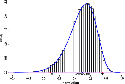
Figure 1: Histogram of $B=10\mbox{,}000$ bootstrap replications for the student score correlation coefficient (4)–(5) scaled to integrate to 1. Solid curve is Fisher’s density formula (6) for $\theta=0.498$. Triangles indicate the exact 95% confidence interval $\theta\in(0.093,0.741)$.

The histogram in Figure 1 compares the distribution of the 10,000 $\theta_{i}$’s with Fisher’s theoretical density function $f_{\theta}(\hat{\theta})$,

$$f_{\theta}(\hat{\theta})=\frac{(n-2)(1-\theta^{2})^{(n-1)/2}(1-\hat{\theta}^{2})^{(n-4)/2}}{\pi}\int_{0}^{\infty}\frac{dw}{(\cosh w-\theta\hat{\theta})^{n-1}},$$ (6)

where $\theta$ has been set equal to its MLE value 0.498. In this sense $f_{0.498}(\cdot)$ is the ideal parametric bootstrap density we would obtain if the number of replications $B$ approached infinity. Chapter 32 of Johnson and Kotz (1970) gives formula (6) and other representations of $f_{\theta}(\hat{\theta})$.

Figure 1 also indicates the exact 95% confidence limits

$$\theta_{0}\in(0.093,0.741),$$ (7)

$2\frac{1}{2}\%$ noncoverage in each tail, obtained from $f_{\theta}(\hat{\theta})$ by the usual construction,

$$\int_{0.498}^{1}f_{0.093}(\theta)\,d\theta=0.025$$ (8)

and similarly at the upper endpoint.

Suppose now we have a prior density $\pi(\theta)$ for the parameter $\theta$ and wish to calculate the posterior density $\pi(\theta|\hat{\theta})$. For any subset $\mathcal{A}$ of the parameter space $\Theta=[-1,1]$,

$$\Pr\{\theta\in\mathcal{A}|\hat{\theta}\}=\int_{\mathcal{A}}\pi(\theta)f_{\theta}(\hat{\theta})\,d\theta\Big{/}\int_{\Theta}\pi(\theta)f_{\theta}(\hat{\theta})\,d\theta$$ (9)

according to Bayes rule.

Define the conversion factor $R(\theta)$ to be the ratio of the likelihood function to the bootstrap density,

$$R(\theta)=f_{\theta}(\hat{\theta})/f_{\hat{\theta}}(\theta).$$ (10)

Here $\hat{\theta}$ is fixed at its observed value 0.498 while $\theta$ represents any point in $\Theta$. We can rewrite (9) as

$$\Pr\{\theta\in\mathcal{A}|\hat{\theta}\}=\frac{\int_{\mathcal{A}}\pi(\theta)R(\theta)f_{\hat{\theta}}(\theta)\,d\theta}{\int_{\Theta}\pi(\theta)R(\theta)f_{\hat{\theta}}(\theta)\,d\theta}.$$ (11)

More generally, if $t(\theta)$ is any function $\theta$, its posterior expectation is

$$E\bigl{\{}t(\theta)|\hat{\theta}\bigr{\}}=\frac{\int_{\Theta}t(\theta)\pi(\theta)R(\theta)f_{\hat{\theta}}(\theta)\,d\theta}{\int_{\Theta}\pi(\theta)R(\theta)f_{\hat{\theta}}(\theta)\,d\theta}.$$ (12)

The integrals in (11) and (12) are now being taken with respect to the parametric bootstrap density $f_{\hat{\theta}}(\cdot)$. Since $\theta_{1},\theta_{2},\ldots,\theta_{B}$ (5) is a random sample from $f_{\hat{\theta}}(\cdot)$, the integrals can be estimated by sample averages in the usual way, yielding the familiar importance sampling estimate of $E\{t(\theta)|\hat{\theta}\}$,

$$\hat{E}\bigl{\{}t(\theta)|\hat{\theta}\bigr{\}}=\sum_{i=1}^{B}t_{i}\pi_{i}R_{i}\Big{/}\sum_{i=1}^{B}\pi_{i}R_{i},$$ (13)

where $t_{i}=t(\theta_{i}),\pi_{i}=\pi(\theta_{i})$, and $R_{i}=R(\theta_{i})$. Under mild regularity conditions, the law of large numbers implies that $\hat{E}\{t(\theta)|\hat{\theta}\}$ approaches $E\{t(\theta)|\theta\}$ as $B\to\infty$. (The accuracy calculations of Section 6 will show that in this case $B=10\mbox{,}000$ was larger than necessary for most purposes.)

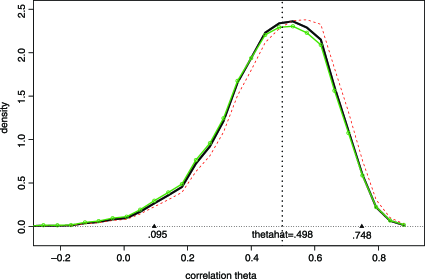
Figure 2: Heavy curve is the posterior density $\pi(\theta|\hat{\theta})$ for the correlation (2), starting from Jeffreys prior (14), obtained by reweighting the $B=10\mbox{,}000$ bootstrap replications (5); triangles show 95% credible limits $\theta_{0}\in(0.095,0.748)$. Light dashed curve is raw unweighted bootstrap distribution. Beaded curve is BCa weighted bootstrap density (17), nearly the same as $\pi(\hat{\theta}|\theta)$ in this case.

The heavy curve in Figure 2 describes $\hat{\pi}(\theta|\hat{\theta})$, the estimated posterior density starting from Jeffreys prior

$$\pi(\theta)=1/\bigl{(}1-\theta^{2}\bigr{)}$$ (14)

(see Section 3). The raw bootstrap distribution puts weight $1/B$ on each of the $B$ replications $\theta_{i}$. By reweighting these points proportionately to $w_{i}=\pi_{i}R_{i}$, we obtain the estimated posterior distribution of $\theta$ given $\hat{\theta}$, with

$$\widehat{\Pr}\{\theta\in\mathcal{A}|\hat{\theta}\}=\sum_{\theta_{i}\in\mathcal{A}}w_{i}\Big{/}\sum_{i=1}^{B}w_{i};$$ (15)

$\hat{\pi}(\theta|\hat{\theta})$ represents the density of this distribution—essentially a smoothed histogram of the 10,000 $\theta_{i}$’s, weighted proportionally to $w_{i}$.

Integrating $\hat{\pi}(\theta|\hat{\theta})$ yields the 95% credible limits ($2\frac{1}{2}\%$ posterior probability in each tail)

$$\theta_{0}\in(0.095,0.748),$$ (16)

close to the exact limits (7). Prior (14) is known to yield accurate frequentist coverage probabilities, being a member of the Welch–Peers family discussed in Section 4.

In this case, the weights $w_{i}=\pi_{i}R_{i}$ can be thought of as correcting the raw unweighted ($w_{i}\equiv 1$) bootstrap density. Figure 2 shows the correction as a small shift leftward. BCa, standing for bias-corrected and accelerated, is another set of corrective weights, obtained from purely frequentist considerations. Letting $\hat{G}(\theta)$ denote the usual empirical cumulative distribution function (c.d.f.) of the bootstrap replications $\theta_{1},\theta_{2},\ldots,\theta_{B}$, the BCa weight on $\theta_{i}$ is

$$w_{i}^{\mathrm{BCa}}=\frac{\varphi(z_{\theta i}/(1+az_{\theta i})-z_{0})}{(1+az_{\theta i})^{2}\varphi(z_{\theta i}+z_{0})}\qquad\bigl{[}z_{\theta i}=\Phi^{-1}\hat{G}(\theta_{i})-z_{0}\bigr{]},$$ (17)

where $\varphi$ and $\Phi$ are the standard normal density and c.d.f., while $z_{0}$ and $a$ are the bias-correction and acceleration constants developed in Efron (1987) and DiCiccio and Efron (1992), further discussed in Section 4 and the Appendix. Their estimated values are $z_{0}=-0.068$ and $a=0$ for the student score correlation problem.

The BCa density $\pi^{\mathrm{BCa}}(\hat{\theta}|\theta)$, obtained by reweighting as in (15), is seen in Figure 2 to nicely agree with the Jeffreys posterior density, being slightly heavier in the left tail, with 95% central interval $\theta_{0}\in(0.074,0.748)$. This agreement is misleadingly soothing, as will be seen in the multidimensional context of Section 4.

3 Exponential families

The Bayes/bootstrap conversion process takes on a simplified form in exponential families. This facilitates its application to multiparameter problems, as discussed here and in the next two sections.

The density functions for a $p$-parameter exponential family $\mathcal{F}$ can be expressed as

$$f_{\beta}(\hat{\beta})=e^{\alpha^{\prime}\hat{\beta}-\psi(\alpha)}f_{0}(\hat{\beta}),$$ (18)

where the $p$-vector $\alpha$ is the canonical parameter, $\hat{\beta}$ is the $p$-dimensional sufficient statistic vector, and where $\psi(\alpha)$, the cumulant generating function, provides the multipliers necessary for $f_{\beta}(\hat{\beta})$ integrating to 1. Here we have indexed the family by its expectation parameter vector $\beta$,

$$\beta=E_{\alpha}\{\hat{\beta}\}$$ (19)

for the sake of subsequent notation, but $\alpha$ and $\beta$ are one-to-one functions and we could just as well write $f_{\alpha}(\hat{\beta})$.

The deviance between any two members of $\mathcal{F}$ is

$$D(\beta_{1},\beta_{2})=2E_{\beta_{1}}\bigl{\{}\log\bigl{(}f_{\beta_{1}}(\hat{\beta})/f_{\beta_{2}}(\hat{\beta})\bigr{)}\bigr{\}}$$ (20)

[denoted equivalently $D(\alpha_{1},\alpha_{2})$ since deviance does not depend on the parameterization of $\mathcal{F}$]. Taking logs in (18) shows that

$$D(\beta_{1},\beta_{2})/2=(\alpha_{1}-\alpha_{2})^{\prime}\beta_{1}-\bigl{(}\psi(\alpha_{1})-\psi(\alpha_{2})\bigr{)}.$$ (21)

Then family (18) can be re-expressed in “Hoeffding’s form” as

$$f_{\beta}(\hat{\beta})=f_{\hat{\beta}}(\hat{\beta})e^{-D(\hat{\beta},\beta)/2}.$$ (22)

Since $D(\hat{\beta},\beta)$ is equal to or greater than zero, (22) shows that $\beta=\hat{\beta}$ is the MLE, maximizing $f_{\beta}(\hat{\beta})$ over all choices of $\beta$ in $\mathcal{B}$, the space of possible expectation vectors.

Parametric bootstrap replications of $\hat{\beta}$ are independent draws from $f_{\hat{\beta}}(\cdot)$,

$$f_{\hat{\beta}}(\cdot)\longrightarrow\beta_{1},\beta_{2},\ldots,\beta_{i},\ldots,\beta_{B},$$ (23)

where $\beta_{i}$ is shorthand notation for $\hat{\beta}_{i}^{*}$. Starting from a prior density $\pi(\beta)$ on $\mathcal{B}$, the posterior expectation of any function $t(\beta)$ given $\hat{\beta}$ is estimated by

$$\hat{E}\bigl{\{}t(\beta)|\hat{\beta}\bigr{\}}=\sum_{i=1}^{B}t(\beta_{i})\pi(\beta_{i})R(\beta_{i})\Big{/}\sum_{i=1}^{B}\pi(\beta_{i})R(\beta_{i})$$ (24)

as in (13), with $R(\beta)$ the conversion factor

$$R(\beta)=f_{\beta}(\hat{\beta})/f_{\hat{\beta}}(\beta).$$ (25)

Note: $\pi(\beta)R(\beta)$ is transformation invariant, so formula (24) produces the same numerical result if we bootstrap $\alpha_{1},\alpha_{2},\ldots,\alpha_{B}$ instead of (23), or for that matter bootstrap any other sufficient vector. See Section 4.

Hoeffding’s form (22) allows a convenient expression for $R(\beta)$:

Lemma 1

Conversion factor (25) equals

$$R(\beta)=\xi(\beta)e^{\Delta(\beta)},$$ (26)

where

$$\xi(\beta)=f_{\hat{\beta}}(\hat{\beta})/f_{\beta}(\beta)$$ (27)

and

$$\Delta(\beta)=\bigl{[}D(\beta,\hat{\beta})-D(\hat{\beta},\beta)\bigr{]}/2.$$ (28)

Letting $\hat{\alpha}$ be the canonical parameter vector corresponding to $\hat{\beta}$, (21) gives

$$\Delta(\beta)=(\alpha-\hat{\alpha})^{\prime}(\beta+\hat{\beta})-2\bigl{[}\psi(\alpha)-\psi(\hat{\alpha})\bigr{]},$$ (29)

which is useful for both theoretical and numerical computations.

The derivatives of $\psi$ with respect to components of $\alpha$ yield the moments of $\hat{\beta}$,

$$\dot{\psi}(\alpha)\equiv(\partial\psi/\partial\alpha_{j})=\beta,\qquad\ddot{\psi}(\alpha)\equiv\bigl{(}\partial^{2}\psi/\partial\alpha_{j}\partial\alpha_{k}\bigr{)}=V(\alpha)=\mathrm{cov}_{\alpha}\{\hat{\beta}\}$$ (30)

and

$$\hskip 1.0pt\dot{\vphantom{\Psi}}\hskip 1.0pt\ddot{\psi}(\alpha)\equiv\bigl{(}\partial^{3}\psi/\partial\alpha_{j}\,\partial\alpha_{k}\,\partial\alpha_{l}\bigr{)}=U(\alpha),$$ (31)

$U_{jkl}(\alpha)=E_{\alpha}(\hat{\beta}_{j}-\beta_{j})(\hat{\beta}_{k}-\beta_{k})(\hat{\beta}_{l}-\beta_{l})$. In repeated sampling situations, where $\hat{\beta}$ is obtained from $n$ independent observations, the entries of $V(\alpha)$ and $U(\alpha)$ are typically of order $O(n^{-1})$ and $O(n^{-2})$, respectively; see Section 5 of Efron (1987).

The normal approximation

$$\hat{\beta}\ \dot{\sim}\ \mathcal{N}_{p}\bigl{(}\beta,V(\alpha)\bigr{)}$$ (32)

yields

$$\qquad f_{\beta}(\beta)\doteq(2\pi)^{-p/2}\bigl{|}V(\alpha)\bigr{|}^{-1/2}\quad\mbox{and}\quad f_{\hat{\beta}}(\hat{\beta})\doteq(2\pi)^{-p/2}\bigl{|}V(\hat{\alpha})\bigr{|}^{-1/2},$$ (33)

so

$$\xi(\beta)\doteq\bigl{|}V(\alpha)\bigr{|}^{1/2}/\bigl{|}V(\hat{\alpha})\bigr{|}^{1/2}.$$ (34)

Because (33) applies the central limit theorem where it is most accurate, at the center, (34) typically errs by a factor of only $1+O(1/n)$ in repeated sampling situations; see Tierney and Kadane (1986). In fact, for discrete families like the Poisson, where $f_{\beta}(\beta)$ is discontinuous, approximation (34) yields superior performance in applications of (26) to (24). In what follows we will treat (34) as exact rather than approximate.

Jeffreys invariant prior density, as described in Kass and Wasserman (1996), takes the form

$$\pi^{\mathrm{Jeff}}(\beta)=c\bigl{|}V(\alpha)\bigr{|}^{-1/2}$$ (35)

in family (18), with $c$ an arbitrary positive constant that does not affect estimates such as (24). Ignoring $c$, we can use (34) and (35) to rewrite the conversion factor $R(\beta)$ (26) as

$$R(\beta)=e^{\Delta(\beta)}/\pi^{\mathrm{Jeff}}(\beta).$$ (36)

Jeffreys prior is intended to be “uninformative.” Like other objective priors discussed in Kass and Wasserman, it is designed for Bayesian use in situations lacking prior experience. Its use amounts to choosing

$$\pi(\beta)R(\beta)=e^{\Delta(\beta)}$$ (37)

in which case (24) takes on a particularly simple form:

Lemma 2

If $\pi(\beta)$ is Jeffreys prior (35), then (24) equals

$$\hat{E}\bigl{\{}t(\beta)|\hat{\beta}\bigr{\}}=\sum_{i=1}^{B}t(\beta_{i})e^{\Delta(\beta_{i})}\Big{/}\sum_{i=1}^{B}e^{\Delta(\beta_{i})}$$ (38)

with $\Delta(\beta)$ as in (28) and (29).

The normal translation model $\hat{\beta}\sim\mathcal{N}_{p}(\beta,\Sigma)$, with $\Sigma$ fixed, has $\Delta(\beta)=0$, so that the Bayes estimate $\hat{t}$ in (38) equals the unweighted bootstrap estimate $\bar{t}$,

$$\hat{t}=\hat{E}\bigl{\{}t(\beta)|\hat{\beta}\bigr{\}}=\sum_{i=1}^{B}t_{i}\Big{/}B=\bar{t}.$$ (39)

Usually though, $\hat{t}$ will not equal $\bar{t}$, the difference relating to the variability of $\Delta(\beta)$ in (38).

A simple but informative result concerns the relative Bayesian difference (RBD) of $t(\beta)$ defined to be

$$\operatorname{RBD}(t)=(\hat{t}-\bar{t})/\overline{\operatorname{sd}}(t),$$ (40)

$\overline{\operatorname{sd}}(t)=[\sum_{1}^{B}(t_{i}-\bar{t})^{2}/B]^{1/2}$:

Lemma 3

Letting $r_{i}=\pi_{i}R_{i}$, the relative Bayesian difference of $t(\beta)$ is

$$\operatorname{RBD}(t)=\overline{\operatorname{cor}}(t,r)\cdot\overline{\operatorname{cv}}(r)$$ (41)

and if $\pi(\beta)=\pi^{\mathrm{Jeff}}(\beta)$,

$$\operatorname{RBD}(t)\doteq\overline{\operatorname{cor}}(t,r)\cdot\overline{\operatorname{sd}}(\Delta);$$ (42)

here $\overline{\operatorname{cor}}(t,r)$ is the empirical correlation between $t_{i}$ and $r_{i}$ for the $B$ bootstrap replications, $\overline{\operatorname{cv}}(r)$ the empirical coefficient of variation of the $r_{i}$ values, and $\overline{\operatorname{sd}}(\Delta)$ the empirical standard deviation of the $\Delta_{i}$ values.

Equation (41) follows immediately from (24),

$$\operatorname{RBD}(t)=\frac{\sum_{1}^{B}(t_{i}-\bar{t})r_{i}/B}{\overline{\operatorname{sd}}(t)\sum_{1}^{B}r_{i}/B}=\overline{\operatorname{cor}}(t,r)\frac{\overline{\operatorname{sd}}(r)}{\bar{r}}.$$ (43)

If $\pi(\beta)$ is the Jeffreys prior (35), then $r(\beta)=\exp(\Delta(\beta))$ (36) and the usual delta-method argument gives $\overline{\operatorname{cv}}(r)\doteq\overline{\operatorname{sd}}(\Delta)$.

The student score example of Figure 2 (which is not in exponential family form) has, directly from definition (40),

$$\operatorname{RBD}(t)=\frac{0.473-0.490}{0.169}=-0.101,$$ (44)

which is also obtained from (41) with $\overline{\operatorname{cor}}(t,r)=-0.945$ and $\overline{\operatorname{cv}}(r)=0.108$. Notice that the $\overline{\operatorname{cv}}(r)$ factor in (41), and likewise $\overline{\operatorname{sd}}(\Delta)$ in (42), apply to any function $t(\beta)$, only the $\overline{\operatorname{cor}}(t,r)$ factor being particular. The multiparameter examples of Sections 3 and 4 have larger $\overline{\operatorname{cv}}(r)$ but smaller $\overline{\operatorname{cor}}(t,r)$, again yielding rather small values of $\operatorname{RBD}(t)$. All of the Jeffreys prior examples in this paper show substantial agreement between the Bayes and unweighted bootstrap results.

Asymptotically, the deviance difference $\Delta(\beta)$ depends on the skewness of the exponential family. A normal translation family has zero skewness, with $\Delta(\beta)=0$ and $R(\beta)=1$, so the unweighted parametric bootstrap distribution is the same as the flat-prior Bayes posterior distribution. In a repeated sampling situation, skewness goes to zero as $n^{-1/2}$, making the Bayes and bootstrap distributions converge at this rate. We can provide a simple statement in one-parameter families:

Theorem 1

In a one-parameter exponential family, $\Delta(\beta)$ has the Taylor series approximation

$$\Delta(\beta)\doteq\tfrac 16\hat{\gamma}Z^{3}\qquad\bigl{[}Z=\hat{V}^{-1/2}(\beta-\hat{\beta})\bigr{]},$$ (45)

where $\hat{V}$ and $\hat{\gamma}$ are the variance and skewness of $\beta\sim f_{\hat{\beta}}(\cdot)$. In large-sample situations, $Z\ \dot{\sim}\ \mathcal{N}(0,1)$ and $\hat{\gamma}$ is $O(n^{-1/2})$, making $\Delta(\beta)$ of order $O_{p}(n^{-1/2})$.

(The proof appears in the Appendix, along with the theorem’s multiparameter version.)

As a simple example, suppose

$$\hat{\beta}\sim\beta\mathrm{Gamma}_{n}/n\qquad\bigl{[}\beta\in(0,\infty)\bigr{]},$$ (46)

so $\hat{\beta}$ is a scaled version of a standard Gamma variate having $n$ degrees of freedom. In this case,

$$\Delta(\beta)\doteq\frac{1}{3\sqrt{n}}Z^{3}\qquad\mbox{with }Z=\sqrt{n}\biggl{(}\frac{\beta}{\hat{\beta}}-1\biggr{)},$$ (47)

making $\Delta(\beta)$ an increasing cubic function of $\beta$. The cubic nature of (45) and (47) makes reweighting of the parametric bootstrap replications $\beta_{i}$ by $\exp(\Delta_{i})$ more extreme in the tails of the distribution than near $\hat{\beta}$.

Stating things in terms of conditional expectations $\hat{E}\{t(\beta)|\hat{\beta}\}$ as in (24) is convenient, but partially obscures the basic idea: that the distribution putting weight proportional to $w_{i}=\pi_{i}R_{i}$ on $\beta_{i}$ approximates the posterior distribution $\pi(\beta|\hat{\beta})$.

As an example of more general Bayesian calculations, consider the “posterior predictive distribution,”

$$g(\mathbf{y})=\int\pi(\beta|\hat{\beta})g_{\beta}(\mathbf{y})\,d\beta,$$ (48)

where $\mathbf{y}$ is the original data set yielding $\hat{\beta}$; by sufficiency as in (3), it has density functions $g_{\beta}(\mathbf{y})=f_{\beta}(\hat{\beta})h(\mathbf{y}|\hat{\beta})$. For each $\beta_{i}$ we sample $\mathbf{y}_{i}^{**}$ from $g_{\beta_{i}}(\cdot)$. Then the discrete distribution putting weight proportional to $w_{i}$ on $\mathbf{y}_{i}^{**}$, for $i=1,2,\ldots,B$, approximates $g(\mathbf{y})$. See Gelman, Meng and Stern (1996).

4 The multivariate normal family

This section and the next illustrate Bayes/bootstrap relationships in two important exponential families: the multivariate normal and generalized linear models. A multivariate normal sample $\mathbf{y}$ comprises $n$ independent $d$-dimensional normal vector observations

$$\mathbf{y}\dvtx y_{i}\stackrel{{\scriptstyle\mathrm{ind}}}{{\sim}}\mathcal{N}_{d}(\mu,\Sigma),\qquad i=1,2,\ldots,n.$$ (49)

This involves $p=d\cdot(d+3)/2$ unknown parameters, $d$ for the mean vector $\mu$ and $d\cdot(d+1)/2$ for the covariance matrix $\Sigma$. We will use $\gamma$ to denote the vector of all $p$ parameters; $\gamma$ is not the expectation vector $\beta$ (19), but rather a one-to-one quadratic function $\gamma=m(\beta)$ described in formula (3.5) of DiCiccio and Efron (1992).

The results of Section 3 continue to hold under smooth one-to-one transformations $\gamma=m(\beta)$. Let $\tilde{f}_{\gamma}(\hat{\gamma})$ denote the density of the MLE $\hat{\gamma}=m(\hat{\beta})$, and likewise $\tilde{R}(\gamma)=\tilde{f}_{\gamma}(\hat{\gamma})/\tilde{f}_{\hat{\gamma}}(\gamma)$ for the conversion factor, $\tilde{D}(\gamma_{1},\gamma_{2})$ for the deviance, $\tilde{\Delta}(\gamma)=[\tilde{D}(\gamma,\hat{\gamma})-\tilde{D}(\hat{\gamma},\gamma)]/2$ for the deviance difference, and $\tilde{\pi}^{\mathrm{Jeff}}(\gamma)$ for Jeffreys prior. Then Lemma 1 continues to apply in the transformed coordinates:

$$\tilde{R}(\gamma)=\tilde{\xi}(\gamma)e^{\tilde{\Delta}(\gamma)}\qquad\bigl{[}\tilde{\xi}(\gamma)=\tilde{f}_{\hat{\gamma}}(\hat{\gamma})/\tilde{f}_{\gamma}(\gamma)\bigr{]}.$$ (50)

(See the Appendix.)

A parametric bootstrap sample

$$\tilde{f}_{\gamma}(\cdot)\longrightarrow\gamma_{1},\gamma_{2},\ldots,\gamma_{B}$$ (51)

approximates the conditional expectation of a function $\tilde{t}(\gamma)$, starting from prior $\tilde{\pi}(\gamma)$, by

$$\hat{E}\bigl{\{}\tilde{t}(\gamma)|\hat{\gamma}\bigr{\}}=\sum_{i=1}^{B}\tilde{t}_{i}\tilde{\pi}_{i}\tilde{R}_{i}\Big{/}\sum_{i=1}^{B}\tilde{\pi}_{i}\tilde{R}_{i}$$ (52)

as in (14), and if $\tilde{\pi}(\gamma)$ is Jeffreys prior,

$$\hat{E}\bigl{\{}\tilde{t}(\gamma)|\hat{\gamma}\bigr{\}}=\sum_{i=1}^{B}\tilde{t}_{i}e^{\tilde{\Delta}_{i}}\Big{/}\sum_{i=1}^{B}e^{\tilde{\Delta}_{i}}$$ (53)

as in (38). This can be particularly handy since $\Delta$ is tranformation invariant and can be evaluated in any convenient set of coordinates, while $\tilde{\pi}^{\mathrm{Jeff}}(\gamma)$ need not be calculated at all.

The following theorem provides $\tilde{\xi}(\gamma)$ and $\tilde{R}(\gamma)$ for a multivariate normal sample (49), working with $\gamma$ the $p=d\cdot(d+3)/2$ coordinates consisting of $\mu$ and the elements of $\Sigma$ on or above its main diagonal:

Theorem 2

In $(\mu,\Sigma)$ coordinates,

$$\tilde{\xi}(\mu,\Sigma)=\bigl{(}|\Sigma|/|\hat{\Sigma}|\bigr{)}^{({d+2})/2}$$ (54)

and

$$\tilde{\Delta}(\mu,\Sigma) = n\biggl{\{}(\mu-\hat{\mu})^{\prime}\frac{\hat{\Sigma}^{-1}-\Sigma^{-1}}{2}(\mu-\hat{\mu})$$

$$\hskip 10.5pt{}+\frac{\operatorname{tr}(\Sigma\Sigma^{n-1}-\hat{\Sigma}\Sigma^{-1})}{2}+\log\frac{|\hat{\Sigma}|}{|\Sigma|}\biggr{\}}.$$

(Proof in the Appendix.)

Here $1/\tilde{\xi}(\mu,\Sigma)$ turns out to be exactly proportional to $|\tilde{V}(\gamma)|^{-1/2}$, and either expression gives $\tilde{\pi}^{\mathrm{Jeff}}(\mu,\Sigma)$. Expression (2) equals the deviance difference (28), no matter what the choice of coordinates.

Theorem 2 makes it easy to carry out parametric bootstrapping: having calculated the usual MLE estimates $(\hat{\mu},\hat{\Sigma})$, each bootstrap data set $\mathbf{y}^{*}$ is generated as in (49),

$$\mathbf{y}^{*}\dvtx y_{i}^{*}\sim\mathcal{N}_{d}(\hat{\mu},\hat{\Sigma}),\qquad i=1,2,\ldots,n,$$ (56)

from which we calculate the bootstrap MLE estimate $(\hat{\mu}^{*},\hat{\Sigma}^{*})$, denoted simply $(\mu,\Sigma)$ as before. To each of $B$ such replicates

$$(\mu,\Sigma)_{1},(\mu,\Sigma)_{2},\ldots,(\mu,\Sigma)_{i},\ldots,(\mu,\Sigma)_{B}$$ (57)

is attached the weight

$$w_{i}=\tilde{\pi}_{i}\tilde{\xi}_{i}e^{\tilde{\Delta}_{i}}$$ (58)

using Theorem 2 (or more exactly $w_{i}/\sum_{1}^{B}w_{j}$); this distribution, supported on the $B$ points (57), estimates the posterior distribution of $(\mu,\Sigma)$ given $(\hat{\mu},\hat{\Sigma})$. Expectations are then obtained as in (52), and similarly for more general posterior parameters such as percentiles and credible limits.

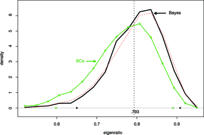
Figure 3: Heavy curve is Bayes posterior density for the eigenratio (59), starting from Jeffreys prior for a bivariate normal model; solid triangles show 95% credible limits $(0.650,0.908)$. Beaded curve is BCa confidence density based on weights (17) with $z_{0}=-0.222,a=0$; BCa 95% interval $(0.598,0.890)$, open triangles, is shifted far leftward. Light dashed curve is unweighted bootstrap density.

Figure 3 applies this methodology to the student score data of Table 1, assuming the bivariate normal model (3). We take the parameter of interest $\theta$ to be the eigenratio

$$\theta=t(\mu,\Sigma)=\lambda_{1}/(\lambda_{1}+\lambda_{2}),$$ (59)

where $\lambda_{1}$ and $\lambda_{2}$ are the ordered eigenvalues of $\Sigma$; $\theta$ has MLE $\hat{\theta}=t(\hat{\mu},\hat{\Sigma})=0.793$.

$B=10\mbox{,}000$ bootstrap replications were generated as in (57), and $t_{i}=t((\mu,\allowbreak\Sigma)_{i})$ calculated for each. Total computation time was about 30 seconds. The heavy curve shows the estimated posterior density of $\theta$ given $(\hat{\mu},\hat{\Sigma})$, starting from Jeffreys prior. The 95% credible region, $2\frac{1}{2}\%$ probability excluded in each tail, was

$$\mbox{{Bayes}:}\quad\theta\in(0.650,0.908).$$ (60)

That is,

$$\sum_{t_{i}\leq 0.650}e^{\tilde{\Delta}_{i}}\Big{/}\sum_{1}^{B}e^{\tilde{\Delta}_{i}}=0.025$$ (61)

and similarly for the upper endpoint.

In this case the BCa 95% confidence limits are shifted sharply leftward compared to (60),

$$\mbox{{BCa}:}\quad\theta\in(0.598,0.890).$$ (62)

The beaded curve in Figure 3 shows the full BCa confidence density, that is, the estimated density based on the BCa weights (17). For the eigenratio, $z_{0}=-0.222$ and $a=0$ are the bias correction and acceleration constants. See the Appendix for a brief discussion of the $z_{0}$ and $a$ calculations.

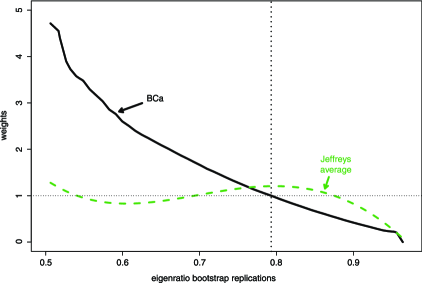
Figure 4: Solid curve: BCa weights (17), with $(z_{0},a)=(-0.222,0)$, plotted versus bootstrap eigenratio replications $\theta_{i}$. Dashed curve: regression of Jeffreys prior Bayes weights $\exp(\tilde{\Delta}_{i})$ on $\theta_{\lambda}$.

Figure 4 helps explain the difference between the Bayes and BCa results. The heavy curve shows the BCa weights (17) increasing sharply to the left as a function of $\theta_{i}=t((\mu,\Sigma)_{i})$, the bootstrap eigenratio values. In other words, smaller values of $\theta_{i}$ are weighted more heavily, pulling the weighted percentile points of the BCa distribution downward. On the other hand, the Bayes weights $\tilde{\pi}^{\mathrm{Jeff}}_{i}\tilde{R}_{i}=\exp(\tilde{\Delta}_{i})$ (represented in Figure 4 by their regression on $\theta_{i}$) are nearly flat, so that the Bayes posterior density is almost the same as the unweighted bootstrap density shown in Figure 3.

The BCa limits are known to yield highly accurate coverage probabilities; see DiCiccio and Efron (1996). Moreover, in the eigenratio case, the MLE $\hat{\theta}$ is strongly biased upward, suggesting a downward shift for the confidence limits. This brings up a familiar complaint against Jeffreys priors, extensively discussed in Ghosh (2011): that in multiparameter settings they can give inaccurate inferences for individual parameters of interest.

This is likely to be the case for any general-purpose recipe for choosing objective prior distributions in several dimensions. For instance, repeating the eigenratio analysis with a standard inverse Wishart prior on $\Sigma$ (covariance matrix $I$, degrees of freedom 2) and a flat prior on $\mu$ gave essentially the same results as in Figure 3. Specific parameters of interest require specifically tailored priors, as with the Bernardo–Berger reference priors, again nicely reviewed by Ghosh (2011).

In fact, the BCa weights can be thought of as providing such tailoring: define the BCa prior (relative to the unweighted bootstrap distribution) to be

$$\pi_{i}^{\mathrm{BCa}}=w_{i}^{\mathrm{BCa}}/R_{i}$$ (63)

with $w_{i}^{\mathrm{BCa}}$ as in (17). This makes the posterior weights $\pi_{i}^{\mathrm{BCa}}R_{i}$ appearing in expressions like (24) equal the BCa weights $w_{i}^{\mathrm{BCa}}$, and makes posterior credible limits based on the $\pi^{\mathrm{BCa}}$ prior equal BCa limits. Formula (63) can be thought of as an automatic device for constructing Welch and Peers’ (1963) “probability matching priors;” see Tibshirani (1989).

Importance sampling methods such as (53) can suffer from excessive variability due to occasional large values of the weights. The “internal accuracy” formula (84) will provide a warning of numerical problems. A variety of helpful counter-tactics are available, beginning with a simple truncation of the largest weight.

Variations in the parametric bootstrap sampling scheme can be employed. Instead of (23), for instance, we might obtain $\beta_{1},\beta_{2},\ldots,\beta_{B}$ from

$$\beta_{i}\stackrel{{\scriptstyle\mathrm{ind}}}{{\sim}}\mathcal{N}_{p}\bigl{(}\hat{\mu}_{\beta},h(\hat{\Sigma}_{\beta})\bigr{)},$$ (64)

where $\hat{\mu}_{\beta}$ and $\hat{\Sigma}_{\beta}$ are the observed mean and covariance of $\beta$’s from a preliminary $f_{\hat{\beta}}(\cdot)$ sample. Here $h(\hat{\Sigma}_{\beta})$ indicates an expansion of $\hat{\Sigma}_{\beta}$ designed to broaden the range of the bootstrap distribution, hence reducing the importance sampling weights. If a regression analysis of the preliminary sample showed the weights increasing in direction $v$ in the $\beta$ space, for example, then $h(\hat{\Sigma}_{\beta})$ might expand $\hat{\Sigma}_{\beta}$ in the $v$ direction. Devices such as this become more necessary in higher-dimensional situations, where extreme variability of the conversion factor $R(\beta_{i})$ may destabilize our importance sampling computations.

Replacing (23) with (64) changes the conversion factor $R(\beta)$ (25), but in an easily computable way. In fact, replacing (23) with $\beta_{i}\sim\mathcal{N}_{p}(\hat{\mu}_{\beta},\hat{\Sigma}_{\beta})$ makes the calculation of $R(\beta)$ easier in situations where there is no simple formula for the bootstrap density $f_{\hat{\beta}}(\beta)$.

5 Generalized linear models

The Bayes/bootstrap conversion theory of Section 3 applies directly to generalized linear models (GLM). A GLM begins with a one-parameter exponential family

$$g_{\eta}(y)=e^{\eta y-\phi(\eta)}g_{0}(y),$$ (65)

where $\eta=\alpha,y=\hat{\beta}$, and $\phi(\eta)=\psi(\alpha)$ in notation (18). An $n\times p$ structure matrix $X$ and a $p$-dimensional parameter vector $\alpha$ then yield an $n$-vector $\bolds{\eta}=X\alpha$, with each entry $\eta_{j}$ governing an independent observation $y_{j}$,

$$y_{j}\stackrel{{\scriptstyle\mathrm{ind}}}{{\sim}}g_{\eta_{j}}(\cdot)\qquad\mbox{for }j=1,2,\ldots,n.$$ (66)

All of this results in a $p$-parameter exponential family (18), with $\alpha$ the canonical parameter vector. Letting $\bolds\mu$ be the expectation vector of $\mathbf{y}=(y_{1},\ldots,y_{n})^{\prime}$,

$$\bolds\mu=E_{\alpha}\{\mathbf{y}\},$$ (67)

the other entries of (18) are

$$\hat{\beta}=X^{\prime}\mathbf{y},\qquad\beta=X^{\prime}\bolds\mu\quad\mbox{and}\quad\psi(\alpha)=\sum_{i=1}^{n}\phi(\mathbf{x}_{j}\alpha),$$ (68)

where $\mathbf{x}_{j}$ is the $j$th row of $X$. The deviance difference $\Delta(\beta)$ (28) has a simple form,

$$\Delta(\beta) = (\alpha-\hat{\alpha})^{\prime}(\beta+\hat{\beta})-2\sum_{j=1}^{n}\bigl{[}\phi(\mathbf{x}_{j}\alpha)-\phi(\mathbf{x}_{j}\hat{\alpha})\bigr{]}$$

$$= (\bolds{\eta}-\hat{\bolds{\eta}})^{\prime}(\bolds\mu+\hat{\bolds\mu})-2\sum_{j=1}^{n}\bigl{[}\phi(\bolds{\eta}_{j})-\phi(\hat{\bolds{\eta}}_{j})\bigr{]}$$

[$\hat{\alpha}$ the MLE of $\alpha$, $\hat{\bolds{\eta}}=X\hat{\alpha}$, and $\hat{\bolds\mu}$ the expectation vector (67) corresponding to $\alpha=\hat{\alpha}$] according to (29).

As an extended example we now consider a microarray experiment discussed in Efron (2010), Section 2.1: 102 men, 50 healthy controls and 52 prostate cancer patients, having each had the activity of $N=6033$ genes measured [Singh et al. (2002)]. A two-sample test comparing patients with controls has been performed for each gene, yielding a $z$-value $z_{k}$, that is, a test statistic having a standard normal distribution under $H_{0k}$, the null hypothesis of no patient/control difference for gene $k$,

$$H_{0k}\dvtx z_{k}\sim\mathcal{N}(0,1).$$ (70)

The experimenters, of course, are interested in identifying nonnull genes.

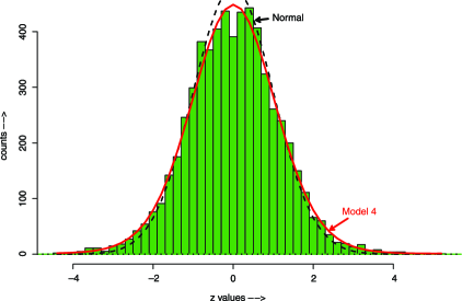
Figure 5: Histogram of the $N=6033$ $z$-values from the prostate cancer study, Singh et al. (2002). Standard normal curve (dashed) is too high at center and too low in the tails. “Model 4,” solid curve, is the fit from a fourth-degree polynomial Poisson regression.

Figure 5 shows a histogram of the $N$ $z$-values. The standard normal curve is too high in the center and too low in the tails, suggesting that at least some of the genes are nonnull. The better-fitting curve “model 4” is a fit from the Poisson regression family discussed next.

There are $J=49$ bins for the histogram, each of width 0.2, with centers $x_{j}$ ranging from $-4.4$ to 5.2. Let $y_{j}$ be the number of $z_{k}$ values in the $j$th bin,

$$y_{j}=\#\{z_{k}\in\operatorname{bin}j\},\qquad j=1,2,\ldots,J=49.$$ (71)

We will assume that the $y_{j}$’s are independent Poisson observations, each having its own expectation $\mu_{j}$,

$$y_{j}\stackrel{{\scriptstyle\mathrm{ind}}}{{\sim}}\operatorname{Poi}(\mu_{j}),\qquad j=1,2,\ldots,J,$$ (72)

and then fit curves to the histogram using Poisson regression. Why this might be appropriate is discussed at length in Efron (2008, 2010), but here we will just take it as a helpful example of the Bayes/bootstrap GLM modeling theory.

We consider Poisson regression models where the canonical parameters $\eta_{j}=\log(\mu_{j})$ are $m$th-degree polynomial functions of the bin centers $x_{j}$, evaluated by glm(y$\sim$poly(x,m),Poisson) in the language R. This is a GLM with the Poisson family, $\eta_{j}=\log\mu_{j}$, where $X$ is a $J\times(m+1)$ matrix having rows $\mathbf{x}_{j}=(1,x_{j},x_{j}^{2},\ldots,x_{j}^{m})$ for $j=1,2,\ldots,J$. For the Poisson distribution, $\phi(\eta)=\mu$ in (65). The deviance difference function (5) becomes

$$\Delta(\beta)=(\bolds{\eta}-\hat{\bolds{\eta}})^{\prime}(\bolds\mu+\hat{\bolds\mu})-2\cdot\mathbf{1}^{\prime}(\bolds\mu-\hat{\bolds\mu})$$ (73)

with $\mathbf{1}$ a vector of $J$ ones.

Table 2: Deviance from Poisson polynomial regression models for counts (71), prostate data; AIC criterion (74) is minimized for the quartic model M4. Boot % shows the proportion of each model selected in $B=4000$ bootstrap replications of the AIC criterion, bootstrapping from M8. Bayes % are weighted Bayes posterior proportions, assuming Jeffreys prior. The St Error column is obtained from the bootstrap-after-bootstrap calculations of Section 6

Model	Deviance	AIC	Boot %	Bayes %	(St Error)
M2	$138.6$	144.6	$0\%$	$0\%$	0(0%)
M3	$137.1$	145.1	$0\%$	$0\%$	0(0%)
M4	$65.3$	75.3	$32\%$	$36\%$	(20%)
M5	$64.3$	76.3	$10\%$	$12\%$	(14%)
M6	$63.8$	77.8	$5\%$	$5\%$	0(8%)
M7	$63.8$	79.8	$1\%$	$2\%$	0(6%)
M8	$59.6$	77.6	$51\%$	$45\%$	(27%)

Let “M$m$” indicate the Poisson polynomial regression model of degree $m$. M2, with $\log(\mu_{j})$ quadratic in $x_{j}$, amounts to a normal location-scale model for the marginal density of the $z_{k}$’s. Higher-order models are more flexible. M4, the quartic model, provided the heavy fitted curve in Figure 5. Table 2 shows the Poisson deviance for the fitted models M2 through M8. A dramatic decrease occurs between M3 and M4, but only slow change occurs after that. The AIC criterion for model $m$,

$$\operatorname{AIC}(m)=\mathrm{Deviance}+2\cdot(m+1)$$ (74)

is minimized at M4, though none of the subsequent models do much worse. The fit from M4 provided the “model 4” curve in Figure 5.

Parametric bootstrap samples $\mathbf{y}^{*}$ were generated from M4, as in (72),

$$\mathbf{y}_{j}^{*}\stackrel{{\scriptstyle\mathrm{ind}}}{{\sim}}\operatorname{Poi}(\hat{\mu}_{j})\qquad\mbox{for }j=1,2,\ldots,J$$ (75)

with $\hat{\mu}_{j}$ the MLE values from M4. $B=4000$ such samples were generated, and for each one the MLE $\hat{\alpha}^{*}$, and also $\hat{\beta}^{*}$ (68), were obtained from the R call glm(y${}^{*}\sim$poly(x,4),Poisson). Using the simplified notation $\alpha=\hat{\alpha}^{*}$ gives bootstrap vectors $\bolds{\eta}=X\alpha,\bolds\mu=\exp(\bolds{\eta})=(\exp(\eta_{j})),\beta=X^{\prime}\mu$, where $X$ is the $49\times 5$ matrix poly(x,4), and finally $\Delta(\beta)$ as in (73). [Notice that $\beta$ represents $\hat{\beta}^{*}$ here, not the “true value” $\beta$ of (68).]

The reweighted bootstrap distribution, with weights proportional to

$$w_{i}=e^{\Delta_{i}}\mbox{ on }\beta_{i}\qquad\mbox{for }i=1,2,\ldots,B=4000,$$ (76)

estimates the posterior distribution of $\beta$ given $\beta_{i}$, starting from Jeffreys prior. The posterior expectation of any parameter $\theta=t(\beta)$ is estimated by $\sum w_{i}t_{i}/\sum w_{i}$ as in (38).

We will focus attention on a false discovery rate (Fdr) parameter $\theta$,

$$\theta(z)=\operatorname{Fdr}(z)=\bigl{[}1-\Phi(z)\bigr{]}/\bigl{[}1-F(z)\bigr{]},$$ (77)

where $\Phi$ is the standard normal c.d.f. and $F(z)$ is the c.d.f. of the Poisson regression model: in terms of the discretized situation (72),

$$F(z)=\sum_{x_{j}\leq z}\mu_{j}\Big{/}\sum_{1}^{J}\mu_{j}$$ (78)

(with a “half count” correction at $z=x_{j}$). $\operatorname{Fdr}(z)$ estimates the probability that a gene having its $z_{k}$ exceeding the fixed value $z$ is nonnull, as discussed, for example, in Efron (2008).

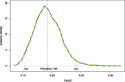
Figure 6: Posterior densities for $\theta=\operatorname{Fdr}(3)$ (77), prostate data, based on $B=4000$ parametric bootstrap replications (75) from the fourth-degree Poisson regression model M4. Solid curve Jeffreys Bayes posterior density, using (76); heavy dashed curve BCa confidence density (17). Both give 95% interval $\theta\in(-0.154,-0.241)$. Light dashed curve is unweighted bootstrap density. Total computation time was about 30 seconds.

Figure 6 concerns the choice $z=3$. Using quartic model M4 to estimate the $\mu_{j}$’s in (78) yields point estimate

$$\hat{\theta}=\widehat{\operatorname{Fdr}}(3)=0.192.$$ (79)

Fdr values near 0.2 are in the “interesting” range where the gene might be reported as nonnull, making it important to know the accuracy of (79).

The $B=4000$ bootstrap samples for M4 (75) yielded bootstrap replications $\theta_{1},\theta_{2},\ldots,\theta_{B}$. Their standard deviation is a bootstrap estimate of standard error for $\hat{\theta},\widehat{\mathrm{se}}=0.024$, so a typical empirical Bayes analysis might report $\widehat{\operatorname{Fdr}}(3)=0.0192\pm 0.024$. A Jeffreys Bayes analysis gives the full posterior density of $\theta$ shown by the solid curve in Figure 6, with 95% credible interval

$$\mbox{M4:}\quad\theta\in(0.154,0.241).$$ (80)

In this case the BCa density (17) [$(z_{0},a)=(-0.047,-0.026)$] is nearly the same as the Bayes estimate, both of them lying just slightly to the left of the unweighted bootstrap density.

The choice of philosophy, Jeffreys Bayes or BCa frequentist, does not make much difference here, but the choice of model does. Repeating the analysis using M8 instead of M4 to generate the bootstrap samples (75) sharply decreased the estimate. Figure 7 compares the bootstrap histograms; the 95% credible interval for $\operatorname{Fdr}(3)$ is now

$$\mbox{M8:}\quad\theta\in(0.141,0.239).$$ (81)

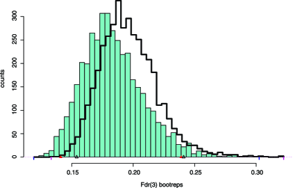
Figure 7: $B=4000$ parametric bootstrap replications of $\operatorname{Fdr}(3)$ from M8 (solid histogram) compared with those from M4 (line histogram). Closed triangles indicate 95% M8 credible limits $(0.141,0.239)$; open triangles M4 limits $(0.154,0.241)$.

AIC calculations were carried out for each of the 4000 M8 bootstrap samples. Of these, 32% selected M4 as the minimizer, compared with 51% for M8, as shown in the Boot % column of Table 2. Weighting each sample proportionally to $\exp(\Delta_{i})$ (76) narrowed the difference to 36% versus 45%, but still with a strong tendency toward M8.

It might be feared that M8 is simply justifying itself. However, standard nonparametric bootstrapping (resampling the $N$ $z_{k}$ values) gave slightly more extreme Boot percentages,

$$\mbox{30\%(M4), 9\%(M5), 4\%(M6), 2\%(M7), 54\%(M8)}.$$ (82)

The fact is that data-based model selection is quite unstable here, as the accuracy calculations of Section 6 will verify.

6 Accuracy

Two aspects of our methodology’s Bayesian estimation accuracy are considered in this section: internal accuracy, the bootstrap sampling error in estimates such as (24) (i.e., how many bootstrap replications $B$ need we take?), and external accuracy, statistical sampling error, for instance, how much would the results in Figure 3 change for a new sample of 22 students? The i.i.d. (independent and identically distributed) nature of bootstrap sampling makes both questions easy to answer.

Internal accuracy is particularly straightforward. The estimate (24) for $\hat{E}\{t(\beta)|\allowbreak\hat{\beta}\}$ can be expressed in terms of $s_{i}=t_{i}\pi_{i}R_{i}$ and $r_{i}=\pi_{i}R_{i}$ as

$$\hat{E}=\bar{s}/\bar{r}\qquad\Biggl{(}\bar{s}=\sum_{1}^{B}s_{i}/B,\bar{r}=\sum_{1}^{B}r_{i}/B\Biggr{)}.$$ (83)

Let $\overline{\mathrm{cov}}$ be the $2\times 2$ empirical covariance matrix of the $B$ vectors $(s_{i},r_{i})$. Then standard delta-method calculations yield a familiar approximation for the bootstrap coefficient of variation of $\hat{E}$,

$$\widehat{\mathrm{cv}}^{2}=\frac{1}{B}\biggl{(}\frac{\bar{c}_{ss}}{\bar{s}^{2}}-2\frac{\bar{c}_{sr}}{\bar{s}\bar{r}}+\frac{\bar{c}_{rr}}{\bar{r}^{2}}\biggr{)},$$ (84)

where $\bar{c}_{ss},\bar{c}_{sr}$ and $\bar{c}_{rr}$ are the elements of $\overline{\mathrm{cov}}$.

The Jeffreys Bayes estimate for eigenratio (59) was $\hat{E}=0.799$ (nearly the same as the MLE 0.793). Formula (84) gave $\widehat{\mathrm{cv}}=0.002$, indicating that $\hat{E}$ nearly equaled the exact Bayes estimate $E\{t(\beta)|\hat{\beta}\}$. $B=10\mbox{,}000$ was definitely excessive. Posterior parameters other than expectations are handled by other well-known delta-method approximations. Note: Discontinuous parameters, such as the indicator of a parameter $\theta$ being less than some value $\theta_{0}$, tend to have higher values of $\widehat{\mathrm{cv}}$.

As far as external accuracy is concerned, the parametric bootstrap can be employed to assess its own sampling error, a “bootstrap-after-bootstrap” technique in the terminology of Efron (1992). Suppose we have calculated some Bayes posterior estimate $\hat{Q}=Q(\hat{\beta})$, for example, $\hat{E}$ or a credible limit, and wonder about its sampling standard error, that is, its frequentist variability. As an answer, we sample $K$ more times from $f_{\hat{\beta}}(\cdot)$,

$$f_{\hat{\beta}}(\cdot)\longrightarrow\hat{\gamma}_{1},\hat{\gamma}_{2},\ldots,\hat{\gamma}_{K},$$ (85)

where the $\gamma$ notation emphasizes that these replications are distinct from $\beta_{1},\beta_{2},\allowbreak\ldots,\beta_{B}$ in (23), the original replications used to compute $\hat{Q}$. Letting $\hat{Q}_{k}=Q(\hat{\gamma}_{k})$, the usual bootstrap estimate of standard error for $\hat{Q}$ is

$$\widehat{\mathrm{se}}(\hat{Q})=\Biggl{[}\sum_{k=1}^{K}(\hat{Q}_{k}-\hat{Q}_{\cdot})^{2}/(K-1)\Biggr{]}^{1/2},$$ (86)

$\hat{Q}_{\cdot}=\sum\hat{Q}_{k}/K$. $K=200$ is usually plenty for reasonable estimation of se$(\hat{Q})$; see Table 6.2 of Efron and Tibshirani (1993).

This recipe looks arduous since each $\hat{Q}_{k}$ requires $B$ bootstrap replications for its evaluation. Happily, a simple reweighting scheme on the original $B$ replications finesses all that computation. Define

$$W_{ki}=f_{\beta_{i}}(\hat{\gamma}_{k})/f_{\beta_{i}}(\hat{\beta}).$$ (87)

Lemma 4

If $\hat{Q}$ is a posterior expectation $\hat{E}=\sum t_{i}\pi_{i}R_{i}/\sum\pi_{i}R_{i}$, then the importance sampling estimate of $\hat{Q}_{k}$ is

$$\hat{Q}_{k}=\sum_{i=1}^{B}t_{i}\pi_{i}R_{i}W_{ki}\Big{/}\sum_{i=1}^{B}\pi_{i}R_{i}W_{ki}$$ (88)

for general quantities $\hat{Q}$, reweighting $\beta_{i}$ proportionately to $\pi_{i}R_{i}W_{i}$ gives $\hat{Q}_{k}$.

The proof of Lemma 4 follows immediately from

$$R_{i}W_{ki}=f_{\beta_{i}}(\hat{\gamma}_{k})/f_{\hat{\beta}}(\beta_{i}),$$ (89)

which is the correct importance sampling factor for converting an $f_{\hat{\beta}}(\beta)$ sample into an $f_{\beta}(\hat{\gamma}_{k})$ likelihood. Note: Formula (88) puts additional strain on our importance sampling methodology and should be checked for internal accuracy, as in (84).

Formula (88) requires no new computations of $t(\beta),\pi(\beta)$ or $R(\beta)$, and in exponential families the factor $W_{ki}$ is easily calculated:

$$W_{ki}=e^{(\alpha_{i}-\hat{\alpha})^{\prime}(\hat{\gamma}_{k}-\hat{\beta})},$$ (90)

where $\alpha_{i}$ is the canonical vector in (18) corresponding to $\beta_{i}$. This usually makes the computation for the bootstrap-after-bootstrap standard error (86) much less than that needed originally for $\hat{Q}$. [Formula (87) is invariant under smooth transformations of $\beta$, and so $W_{ki}$ can be calculated directly in other coordinate systems as a ratio of densities.]

A striking use of (86) appears in the last two columns of Table 2, Section 5. Let $t_{4}(\beta_{i})$ be the indicator function of whether or not model 4 minimized AIC for the $i$th bootstrap replication: $\hat{E}\{t_{4}(\beta)|\hat{\beta}\}=0.36$ according to the Bayes % column. However, its bootstrap-after-bootstrap standard error estimate was $\widehat{\mathrm{se}}=0.20$, with similarly enormous standard errors for the other model selection probabilities. From a frequentist viewpoint, data-based model selection will be a highly uncertain enterprise here.

Frequentist assessment of objective Bayes procedures has been advocated in the literature, for example, in Berger (2006) and Gelman, Meng and Stern (1996), but seems to be followed most often in the breach. The methodology here can be useful for injecting a note of frequentist caution into Bayesian data analysis based on priors of convenience.

If our original data set $\mathbf{y}$ consists of $n$ i.i.d. vectors $y_{i}$, as in Table 1, we can jackknife instead of bootstrapping the $\hat{\gamma}_{k}$’s. Now $\hat{\gamma}_{k}$ is $\hat{\beta}$ recomputed from the data set $\mathbf{y}_{(i)}$ having $y_{i}$ removed for $k=1,2,\ldots,n$. Formulas (87)–(90) still hold, yielding

$$\widehat{\mathrm{se}}_{\mathrm{jack}}=\Biggl{[}\frac{n-1}{n}\sum_{k=1}^{n}(\hat{Q}_{k}-\hat{Q}_{\cdot})^{2}\Biggr{]}^{1/2}.$$ (91)

An advantage of jackknife resampling is that the $\hat{\gamma}_{k}$ values lie closer to $\hat{\beta}$, making $W_{ki}$ closer to 1 and putting less strain on the importance sampling formula (88).

7 Summary

The main points made by the theory and examples of the preceding sections are as follows:

• The parametric bootstrap distribution is a favorable starting point for importance sampling computation of Bayes posterior distributions (as in Figure 2).

• This computation is implemented by reweighting the bootstrap replications rather than by drawing observations directly from the posterior distribution as with MCMC [formulas (24), (25)].

• The necessary weights are easily computed in exponential families for any prior, but are particularly simple starting from Jeffreys invariant prior, in which case they depend only on the deviance difference $\Delta(\beta)$ [(26)–(29), (38), (2), (5)].

• The deviance difference depends asymptotically on the skewness of the family, having a cubic normal form (46).

• In our examples, Jeffreys prior yielded posterior distributions not much different than the unweighted bootstrap distribution. This may be unsatisfactory for single parameters of interest in multiparameter families (Figure 3).

• Better uninformative priors, such as the Welch–Peers family or reference priors, are closely related to the frequentist BCa reweighting formula [(17), Figures 2 and 6].

• Because of the i.i.d. nature of bootstrap resampling, simple formulas exist for the accuracy of posterior computations as a function of the number $B$ of bootstrap replications. [Importance sampling methods can be unstable, so internal accuracy calculations, as suggested following (84), are urged.] Even with excessive choices of $B$, computation time was measured in seconds for our examples (84).

• An efficient second-level bootstrap algorithm (“bootstrap-after-bootstrap”) provides estimates for the frequentist accuracy of Bayesian inferences [(85)–(88)].

• This can be important in assessing inferences based on formulaic priors, such as those of Jeffreys, rather than on genuine prior experience (last column, Table 2 of Section 5).

Appendix

Transformation of coordinates: Let $J(\beta)$ be the Jacobian of the transformation $\gamma=m(\beta)$, that is, the absolute value of the determinant of the Hessian matrix $(\partial\beta_{i}/\partial\gamma_{j})$. Then $\tilde{f}_{\gamma}(\hat{\gamma})=f_{\beta}(\hat{\beta})J(\hat{\beta})$ gives

$$\tilde{\xi}(\gamma)=\frac{f_{\hat{\beta}}(\hat{\beta})J(\hat{\beta})}{f_{\beta}(\beta)J(\beta)}=\xi(\beta)\frac{J(\hat{\beta})}{J(\beta)}$$ (92)

in (50), and

$$\tilde{R}(\gamma) = \frac{\tilde{f}_{\gamma}(\hat{\gamma})}{\tilde{f}_{\hat{\gamma}}(\gamma)}=\frac{f_{\beta}(\hat{\beta})}{f_{\hat{\beta}}(\beta)}\frac{J(\hat{\beta})}{J(\beta)}=R(\beta)\frac{J(\hat{\beta})}{J(\beta)}$$

$$= \xi(\beta)e^{\Delta(\beta)}\frac{J(\hat{\beta})}{J(\beta)}=\tilde{\xi}(\gamma)e^{\tilde{\Delta}(\gamma)},$$

since $\tilde{\Delta}(\gamma)=\Delta(\beta)$ by the transformation invariance of the deviance.

For any prior density $\pi(\beta)$ we have $\tilde{\pi}(\gamma)=\pi(\beta)J(\beta)$ and

$$\tilde{\pi}(\gamma)\tilde{R}(\gamma) = \pi(\beta)J(\beta)R(\beta)J(\hat{\beta})/J(\beta)$$

$$= J(\hat{\beta})\pi(\beta)R(\beta).$$

$J(\hat{\beta})$ acts as a constant in (Appendix), showing that (52) is identical to (24). This also applies to Jeffreys prior, $\tilde{\pi}^{\mathrm{Jeff}}(\gamma)$, which by design is transformation invariant, yielding (53). Proof of Theorem 1 In a one-parameter exponential family, (30) and (31) give

$$\psi(\alpha)-\psi(\hat{\alpha})\doteq\hat{\beta}\,d\alpha+\hat{V}(d\alpha)^{2}/2+\hat{U}(d\alpha)^{3}/6$$ (95)

and

$$\beta-\hat{\beta}\doteq\hat{V}\,d\alpha+\hat{U}(d\alpha)^{2}/2,$$ (96)

where $d\alpha=\alpha-\hat{\alpha},\hat{V}=V(\hat{\alpha})$, and $\hat{U}=U(\hat{\alpha})$. Expression (29) for $\Delta$ can be written as

$$\Delta=(\beta-\hat{\beta})\,d\alpha+2\bigl{[}\hat{\beta}\,d\alpha-(\psi-\hat{\psi})\bigr{]}.$$ (97)

Applying (95) and (96) reduces (97) to

$$\Delta \doteq \tfrac 16\hat{U}(d\alpha)^{3}=\tfrac 16\hat{\gamma}\bigl{[}\hat{V}^{1/2}(\alpha-\hat{\alpha})\bigr{]}^{3}$$

$$\doteq \tfrac 16\hat{\gamma}\bigl{[}\hat{V}^{-1/2}(\beta-\hat{\beta})\bigr{]}^{3}=\tfrac 16\hat{\gamma}Z^{3}$$

with $\hat{\gamma}=\hat{U}/\hat{V}^{3/2}$ the skewness, the last line following from $Z\equiv\hat{V}^{-1/2}(\beta-\hat{\beta})\doteq\hat{V}^{1/2}(\alpha-\hat{\alpha})$ (96). Standard exponential family theory shows that $Z\to\mathcal{N}(0,1)$ under repeated sampling, verifying the theorem [remembering that the asymptotics here are for $\beta\sim f_{\hat{\beta}}(\cdot)$, with $\hat{\beta}$ fixed]. The skewness $\hat{\gamma}$ is then $O(n^{-1/2})$, making $\Delta$ of order $O_{p}(n^{-1/2})$. The first missing term in the Taylor expansion (Appendix) for $\Delta$ is $\hat{\delta}Z^{4}/12$, $\hat{\delta}$ the kurtosis, and is of order $O_{p}(n^{-1})$.

The multiparameter version of Theorem 1 begins by considering a one-parameter subfamily of (18) now indexed by $\alpha$ rather than $\beta$,

$$f_{a}^{(v)}(\hat{\beta})=f_{\hat{\alpha}+av}(\hat{\beta})=e^{(\hat{\alpha}+av)^{\prime}\hat{\beta}-\psi(\hat{\alpha}+av)}f_{0}(\hat{\beta}),$$ (99)

where $v$ is some fixed vector in $\mathbb{R}^{p}$; $a$ here is not connected with that in (17). The deviance difference within $f_{a}^{(v)}$ is

$$\Delta^{(v)}(a)=\Delta(\hat{\alpha}+av)$$ (100)

since deviance is entirely determined by the two densities involved.

The exponential family terms (18) for family $f_{a}^{(v)}(\cdot)$ are

$$\alpha^{(v)} = a,\qquad\hat{\beta}^{(v)}=v^{\prime}\hat{\beta},\qquad\beta^{(v)}=v^{\prime}\beta,$$

$$\hat{V}^{(v)} = v^{\prime}\hat{V}v\quad\mbox{and}\quad\hat{U}^{(v)}=\sum_{j=1}^{p}\sum_{k=1}^{p}\sum_{l=1}^{p}\hat{U}_{jkl}v_{j}v_{k}v_{l},$$

giving skewness $\hat{\gamma}^{(v)}=\hat{U}^{(v)}/\hat{V}^{(v)3/2}$. Applying the one-dimensional result gives

$$\Delta(\hat{\alpha}+av)\doteq\frac{1}{6}\hat{\gamma}^{(v)}{Z^{(v)3}}\qquad\mbox{with }Z^{(v)}=\frac{v^{\prime}(\beta-\hat{\beta})}{(v^{\prime}\hat{V}v)^{1/2}}.$$ (102)

Since $v$ can be any vector, (102) describes the asymptotic form of $\Delta(\cdot)$ in the neighborhood of $\hat{\alpha}$. Proof of Theorem 2 For a single observation $y\sim\mathcal{N}_{d}(\mu,\Sigma)$, let $f_{1}$ and $f_{2}$ represent its density under $(\mu_{1},\Sigma_{1})$ and $(\mu_{2},\Sigma_{2})$, respectively. Then

$$2\log\frac{f_{1}(y)}{f_{2}(y)} = \log\frac{|\Sigma_{1}|}{|\Sigma_{2}|}+(y-\mu_{2})^{\prime}\Sigma_{2}(y-\mu_{2})$$

$${}-(y-\mu_{1})^{\prime}\Sigma_{1}(y-\mu_{1}).$$

But if $y\sim\mathcal{N}_{d}(\mu_{1},\Sigma_{1})$,

$$E_{f_{1}}\bigl{\{}(y-\mu_{2})^{\prime}\Sigma_{2}^{-1}(y-\mu_{2})\bigr{\}}$$

(104)

$$\qquad=(\mu_{2}-\mu_{1})^{\prime}\Sigma_{2}^{-1}(\mu_{2}-\mu_{1})+\operatorname{tr}\Sigma_{1}\Sigma_{2}^{-1}$$

while $E_{f_{1}}\{(y-\mu_{1})^{\prime}\Sigma_{1}^{-1}(y-\mu_{1})\}=d$. Taking the $f_{1}$ expectation of (Appendix) gives the deviance

$$D\bigl{(}(\mu_{1},\Sigma_{1}),(\mu_{2},\Sigma_{2})\bigr{)}$$

$$\qquad=\log|\Sigma_{2}|/|\Sigma_{1}|+(\mu_{2}-\mu_{1})^{\prime}\Sigma_{2}^{-1}(\mu_{2}-\mu_{1})+\operatorname{tr}\Sigma_{1}\Sigma_{2}^{-1}-d$$

for sample size $n=1$. The deviance difference for sample size $n$

$$\Delta=\frac{n}{2}\bigl{\{}D\bigl{(}(\mu,\Sigma),(\hat{\mu},\hat{\Sigma})\bigr{)}-D\bigl{(}(\hat{\mu},\hat{\Sigma}),(\mu,\Sigma)\bigr{)}\bigr{\}}$$ (106)

is then seen to equal (2).

The density of $(\hat{\mu},\hat{\Sigma})$ from a $\mathcal{N}_{p}(\mu,\Sigma)$ sample of size $n$ is proportional to

$$\bigl{\{}|\Sigma|^{-1/2}e^{-{n}(\hat{\mu}-\mu)^{\prime}\Sigma^{-1}(\hat{\mu}-\mu)/2}\bigr{\}}\bigl{\{}|\hat{\Sigma}|^{({n-d-2})/2}e^{-{n}\operatorname{tr}\Sigma^{-1}\hat{\Sigma}/2}/|\Sigma|^{({n-1})/2}\bigr{\}}$$ (107)

yielding (54).

The BCa weights: The BCa system of second-order accurate bootstrap confidence intervals was introduced in Efron (1987) (Section 2 giving an overview of the basic idea) and restated in weighting form (17) in Efron and Tibshirani (1998). The bias correction constant $z_{0}$ is obtained directly from the MLE $\hat{\theta}$ and the bootstrap replication $\theta_{1},\theta_{2},\ldots,\theta_{B}$ according to

$$z_{0}=\Phi^{-1}\bigl{(}\#\{\theta_{i}\leq\hat{\theta}\}/B\bigr{\}}.$$ (108)

DiCiccio and Efron (1992) discuss “ABC” algorithms for computing $a$, the acceleration constant. The program abc2 is available in the supplement to this article. It is very fast and accurate, but requires individual programming for each exponential family. A more computer-intensive R program, accel, which works directly from the bootstrap replications $(\beta_{i},t_{i})$ [as in (23) and (24)], is also available in the supplement.

=210pt $\bolds{\hat{\theta}}$ $\bolds{z_{0}}$ $\bolds{a}$ Student correlation 0.498 $-0.069$ $0$ Student eigenratio 0.793 $-0.222$ $0$ Prostate data Fdr(3) 0.192 $-0.047$ $-0.026$

Table 3: BCa constants $z_{0}$ and $a$ for our three examples

Table 3 shows $z_{0}$ and $a$ for our three main examples. Notice the especially large bias correction needed for the eigenratio.

References

• Berger (2006) {barticle}[mr] \bauthor\bsnmBerger, \bfnmJames\binitsJ. (\byear2006). \btitleThe case for objective Bayesian analysis. \bjournalBayesian Anal. \bvolume1 \bpages385–402. \bidissn=1936-0975, mr=2221271 \bptokimsref \endbibitem