Spin coherent states in NMR quadrupolar system: experimental and theoretical applications

Abstract

Working with nuclear magnetic resonance (NMR) in quadrupolar spin systems, in this paper we transfer the concept of atomic coherent state to the nuclear spin context, where it is referred to as pseudo-nuclear spin coherent state (pseudo-NSCS). Experimentally, we discuss the initialization of the pseudo-NSCSs and also their quantum control, implemented by polar and azimuthal rotations. Theoretically, we compute the geometric phases acquired by an initial pseudo-NSCS on undergoing three distinct cyclic evolutions: $i)$ the free evolution of the NMR quadrupolar system and, by analogy with the evolution of the NMR quadrupolar system, that of $ii)$ single-mode and $iii)$ two-mode Bose-Einstein Condensate like system. By means of these analogies, we derive, through spin angular momentum operators, results equivalent to those presented in the literature for orbital angular momentum operators. The pseudo-NSCS description is a starting point to introduce the spin squeezed state and quantum metrology into nuclear spin systems of liquid crystal or solid matter.

I Introduction

In a seminal work, R. J. Glauber glauber1963 proposed the concept of a coherent state as an eigenstate of the annihilation operator of the harmonic oscillator. This concept was extended to atoms as the well-known atomic coherent states (ACS) arecchi1972 ; perelomov . These coherent states, used in many physical processes in the fields of quantum electrodynamics raimond2001 , trapped ions leibfried2003 and Bose-Einstein condensates (BECs) leggett2001 , are of fundamental importance because they minimize the Heisenberg uncertainty arecchi1972 . The minimization of uncertainty tends to amplify the quantum effects on the macroscopic scale. One physical system that manifests quantum effects at a macroscopic level is the BEC. In this connection, an interesting application of the ACS was developed by Chen et al. chen2004 , who computed geometric phases of a coupled two-mode BEC system for an adiabatic and cyclic time evolution. Other applications are the generation of macroscopic quantum superpositions gordon1999 and dynamic control bargill2009 ; grond2009 in BECs.

The topic of geometric phase has recently received considerable attention and it has been employed increasingly in quantum information processing jones2000 ; ota2009PRA1 ; chen2009 ; niu2010 . The quantum version of geometric phases was first reported and studied by M.V. Berry in the 1980’s berry1984 and implemented, thereafter, in many physical systems tomita1986 ; bhandari1988 ; leek2007 . A general discussion of geometric phases acquired by pure states was published by N. Mukunda and R. Simon mukunda1993 . In this new approach, the authors took advantage of quantum kinematic concepts, so that this formalism could be applied in a general context, such as in any smooth open path defined by unit vectors in a Hilbert space. Many applications using this formalism have appeared, for instance in noncyclic geometric quantum computation wang2009 and, more recently, nonadiabatic geometric quantum gates using composite pulses ota2009PRA1 , both of these applications being discussed in the NMR context. Other applications of the Mukunda-Simon approach have been the study of geometric phases in a nonstationary superposition of atomic states induced by an engineered reservoir prado2009 , and also the study of the effect of geometric phases on the pseudospin dynamics of two coupled BECs duzzioni2007 and of a spin-orbit-coupled BEC larson2009 . Likewise, NMR experiments in systems with two coupled spins and quadrupolar spin systems have been published, in which the geometric phase of an adiabatic cyclic evolution of an initial quantum state is analyzed suter1987 . Other potential NMR applications of adiabatic jones2000 ; ekert2000 and nonadiabatic xiang2001 ; zhu2002A ; zhu2002B geometric quantum computation have also been reported.

These advances inspired us to study two subjects related to NMR quadrupolar systems. The first is the possibility of transferring the definition of ACS to a nuclear spin state, which will be referred to as a pseudo-nuclear spin coherent state (pseudo-NSCS). The second concerns an application of pseudo-NSCSs to compute geometric phases in three different configurations: $i)$ the free evolution of the NMR quadrupolar system abragam1994 and, by analogy of the evolutions of the NMR quadrupolar system, that of $ii)$ single- and $iii)$ two-mode BEC-like system auccaise2009 ; milburn1997 . Under this cyclic evolution, we apply the Mukunda and Simon formalism and obtained theoretical results analogous to those of Zhang et al. in Ref. zhang2006PRL . Special attention was given to configurations $ii)$ and $iii)$, in which we took the advantage of the mapping between the quasiparticle description and pseudo-spin momentum operators for any spin value $I$.

In general, the present paper presents experimental results and theoretical applications of the mapping between the atomic and nuclear spin scenarios. This will be a basis for future experimental implementations of quantum control, and also to establish an NMR quadrupolar system as a workbench for a BEC system.

This paper is organized as follows: In section II, the main concepts and a review of ACS are presented, while in section III the NMR quadrupolar system is briefly described. Section IV is devoted to the experimental procedure to initialize the pseudo-NSCSs and describes the quantum control of polar and azimuthal rotations. In section V, theoretical applications of the pseudo-NSCS based on the geometric phase concept are elaborated for configurations $i)$, $ii)$ and $iii)$ and in section VI we report our conclusions.

II Atomic coherent states

In the theory of ACS, a Bloch vector $\mathbf{n}=\left(\sin\theta\cos\varphi,\right.$ $\left.\sin\theta\sin\varphi,\cos\theta\right)$ is transformed by the action of a rotation operator $\mathbf{R}_{\theta,\varphi}=e^{-i\theta\left(\mathbf{J}\cdot\mathbf{m}\right)}$. The operator $\mathbf{R}_{\theta,\varphi}$ represents a rotation of angle $\theta$ around an axis defined by $\mathbf{m}=\left(\sin\varphi,-\cos\varphi,0\right)$, where $\mathbf{J\cdot m}=\mathbf{J}_{x}\sin\varphi-\mathbf{J}_{y}\cos\varphi$. The operator $\mathbf{J}$ signifies the total angular momentum, with components $\mathbf{J}_{x}$, $\mathbf{J}_{y}$, and $\mathbf{J}_{z}$, such that $j$ is the total angular momentum quantum number and its projection corresponds to $m=-j,-j+1,\ldots,j-1,j$. After a simple algebraic procedure, the application of $\mathbf{R}_{\theta,\varphi}$ to the fundamental state denoted by $\left|j,-j\right\rangle$ produces an excited state represented by perelomov ; inomata ; arecchi1972 :

$$\left|\zeta\left(\theta,\varphi\right)\right\rangle = \mathbf{R}_{\theta,\varphi}\left|j,-j\right\rangle=\frac{1}{\left(1+\zeta^{\ast}\zeta\right)^{j}}e^{\zeta\mathbf{J}_{+}}\left|j,-j\right\rangle\text{,}$$ (1)

$$= \sum_{m=-j}^{j}\frac{\zeta^{j+m}}{\left(1+\zeta^{\ast}\zeta\right)^{j}}\sqrt{\frac{\left(2j\right)!}{\left(j+m\right)!\left(j-m\right)!}}\left|j,m\right\rangle\text{,}$$

where $\zeta=-e^{-i\varphi}\tan\frac{\theta}{2}$, with the angles $\varphi$ and $\theta$ as shown in Fig. 1, while $\mathbf{J}_{\pm}=\mathbf{J}_{x}\pm i\mathbf{J}_{y}$, and $\left|j,m\right\rangle$ are eigenstates of the operator $\mathbf{J}_{z}$, with eigenvalues $m\hbar$. The complex phase that characterizes the ACS may be defined in the complex plane $Z$ (Greek capital $\zeta$) or over the Bloch sphere, where the ground state is represented by the south pole and the most excited state is identified with the north pole.

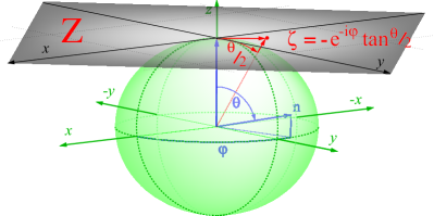
Figure 1: (Color online) For a nuclear spin system we define rotation angles $\theta$ and $\varphi$ on the Bloch sphere relative to the $\mathbf{xyz}$ frame and  the corresponding value of $\zeta$ in the complex plane denoted by $Z$, the Greek capital form of $\zeta$. The north pole corresponds to $\zeta=0$ and the south pole to $\zeta=\infty$.

Let us consider the density operator of the ACS denoted by $\rho=\left|\zeta\left(\theta,\varphi\right)\right\rangle\left\langle\zeta\left(\theta,\varphi\right)\right|$ $=\sum_{m,m^{\prime}=-j}^{j}\rho_{m,m^{\prime}}\left|j,m\right\rangle\left\langle j,m^{\prime}\right|$. From Eq. (1), each element of $\rho$ is given by

$$\rho_{m,m^{\prime}} = (-1)^{2j+m+m^{\prime}}e^{i(m^{\prime}-m)\varphi}\cos^{2j-m-m^{\prime}}\left(\theta/2\right)\sin^{2j+m+m^{\prime}}\left(\theta/2\right)$$ (2)

$$\times\sqrt{\frac{\left(2j\right)!}{\left(j+m^{\prime}\right)!\left(j-m^{\prime}\right)!}}\sqrt{\frac{\left(2j\right)!}{\left(j+m\right)!\left(j-m\right)!}}\text{.}$$

Hence, if the angular parameters $\theta$ and $\varphi$ are known, the amplitude of each element $\rho_{m,m^{\prime}}$ can be obtained. The inverse procedure, that is, the computation of $\theta$ and $\varphi$ from the elements $\rho_{m,m^{\prime}}$, is also possible. In the case of $\theta$, we use

$$\begin{array}[]{ccc}\sqrt[4j]{\rho_{j,j}}&=&\sin\frac{\theta}{2}\text{,}\\ \sqrt[4j]{\rho_{-j,-j}}&=&\cos\frac{\theta}{2}\text{,}\end{array}$$ (3)

for any value of $j$. In the case of $\varphi$, when $j$ is an integer

$$\frac{\left(\rho_{0,1}+\rho_{1,0}\right)\sqrt{\left(j+1\right)!\left(j-1\right)!}\left(j\right)!}{2\left(-1\right)^{2j+1}\left(\cos\frac{\theta}{2}\right)^{2j-1}\left(\sin\frac{\theta}{2}\right)^{2j+1}\left(2j\right)!} = \cos\varphi\text{,}$$ (4)

$$\frac{\left(\rho_{0,1}-\rho_{1,0}\right)\sqrt{\left(j+1\right)!\left(j-1\right)!}\left(j\right)!}{2i\left(-1\right)^{2j+1}\left(\cos\frac{\theta}{2}\right)^{2j-1}\left(\sin\frac{\theta}{2}\right)^{2j+1}\left(2j\right)!} = \sin\varphi\text{.}$$ (5)

Similar expressions can be obtained in terms of the density matrix elements $\rho_{0,-1}$ and $\rho_{-1,0}$ (not shown). For $j$ a half integer, these equations become

$$\frac{\left(\rho_{\frac{-1}{2},\frac{1}{2}}+\rho_{\frac{1}{2},\frac{-1}{2}}\right)\left(j-\frac{1}{2}\right)!\left(j+\frac{1}{2}\right)!}{2\left(-1\right)^{2j}\left(\cos\frac{\theta}{2}\right)^{2j}\left(\sin\frac{\theta}{2}\right)^{2j}\left(2j\right)!} = \cos\varphi\text{,}$$ (6)

$$\frac{\left(\rho_{\frac{-1}{2},\frac{1}{2}}-\rho_{\frac{1}{2},\frac{-1}{2}}\right)\left(j-\frac{1}{2}\right)!\left(j+\frac{1}{2}\right)!}{2i\left(-1\right)^{2j}\left(\cos\frac{\theta}{2}\right)^{2j}\left(\sin\frac{\theta}{2}\right)^{2j}\left(2j\right)!} = \sin\varphi\text{.}$$ (7)

Therefore a general ACS given by (1) is completely characterized by $j$, $\theta$, and $\varphi$.

III NMR quadrupolar systems

NMR quadrupolar systems are composed of nuclei with spin $I>1/2$ subjected to both a magnetic field and an electric field gradient, where the nuclear magnetic moment is quantized as $M=I,I-1,...,-I$. Considering also the interaction with a radio frequency (RF) field used for excitation, in a reference frame rotating around $z$-axis with angular velocity $\omega_{RF}$, the NMR Hamiltonian can be written (for more details see section VII of Ref. abragam1994 ):

$$\mathcal{H}_{NMR} = -\hbar\left(\omega_{L}-\omega_{RF}\right)\mathbf{I}_{z}+\hbar\frac{\omega_{Q}}{6}\left(3\mathbf{I}_{z}^{2}-\mathbf{I}^{2}\right)$$ (8)

$$+\hbar\omega_{1}\left(\mathbf{I}_{x}\cos\varphi_{s}+\mathbf{I}_{y}\sin\varphi_{s}\right)+\mathcal{H}_{env}\text{,}$$

where $\mathbf{I}_{x}$, $\mathbf{I}_{y}$, $\mathbf{I}_{z}$ are the $x,y,z$ components of the total spin angular momentum operator. The first term of the Hamiltonian is due to the interaction of the nuclear magnetic moments with the strong magnetic field $B_{0}$ (Zeeman term). The second is due to the interaction of the quadrupole moments of the nuclei with the internal electric field gradient. $\left(\omega_{L}\right)$ and $\left(\omega_{Q}\right)$ stand for the Larmor and Quadrupolar frequencies (coupling strengths), which in this case, satisfy the inequality $\left|\omega_{Q}\right|\ll\left|\omega_{L}\right|$. The third term represents the external time-dependent RF field perturbation of intensity $B_{1}=\omega_{1}/\gamma$, applied along the direction of the corresponding vector $\mathbf{m}$, with $\gamma$ being the gyromagnetic ratio. The fourth term represents weak interactions between quadrupolar nuclei and other nuclei, electrons, random fields, referred to here as environment. This term will be neglected as its contribution is weak oliveira2007 .

A quadrupolar system in the rotating frame will be used to describe two different  situations. In  the  first, the external time-dependent perturbation is  present, with $\left|\omega_{L}\right|\cong\left|\omega_{RF}\right|$, and $\left|\omega_{1}\right|>>\left|\omega_{Q}\right|$ specifies a regime where the perturbation equally affects all energy levels of the system, non-selective pulse; the evolution operator is then given by

$$\mathcal{U}_{RF}\cong\exp\left[-i\omega_{1}t\left(\mathbf{I}_{x}\cos\varphi_{s}+\mathbf{I}_{y}\sin\varphi_{s}\right)\right]\text{.}$$ (9)

The physical parameters to be identified are the polar $\left(\theta\right)$ and azimuthal $\left(\varphi\right)$ angles defining the rotation operator $\mathbf{R}_{\theta,\varphi}$. From the RF operator $\mathcal{U}_{RF}\left(t\right)$, these angles are

$$\theta \equiv \omega_{1}t\text{,}$$ (10)

$$\varphi \equiv \varphi_{s}+\frac{\pi}{2}\text{.}$$ (11)

Secondly, when the external RF perturbation is absent, the corresponding evolution operator is

$$\mathcal{U}_{Ev}=\exp\left[i\left(\omega_{L}-\omega_{RF}\right)t\mathbf{I}_{z}-\frac{i\omega_{Q}t}{6}\left(3\mathbf{I}_{z}^{2}-\mathbf{I}^{2}\right)\right]\text{,}$$ (12)

which refers to a free evolution regime. Note that the operator $\mathcal{U}_{Ev}$ cannot be written as a rotation operator $\mathbf{R}_{\theta,\varphi}$, since it is not generated by the vectors $\mathbf{n}$ and $\mathbf{m}$ (see section II). This approach is similar to that discussed by Kitagawa and Ueda kitagawa1993 in the study of spin squeezed states.

IV Experimental implementation of the pseudo-NSCS

The NMR experiments were carried out at room temperature in a VARIAN INOVA 400 MHz spectrometer. The pseudo-NSCS was implemented with the ²³Na nuclei ($I=3/2$) present in sodium dodecil sulfate (SDS) in a lyotropic liquid crystal, prepared with $21.3$ wt % SDS, $3.7$ wt % decanol, and $75$ wt % D₂O. The strength of the Larmor frequency and quadrupolar couplings were 105.85 MHz and 15 kHz, respectively. Typical $\pi$-pulse lengths of 8 $\mu$s and recycle delays of 500 ms were used. The T₂ and T₁ relaxation times of the ²³Na nuclear spins are $2.6\pm 0.3$ ms and $12.2\pm 0.2$ ms, respectively.

Room temperature thermal equilibrium NMR systems are almost maximum mixture states, represented by a density matrix which deviates only slightly from the normalized identity matrix

$$\rho\approx\frac{\left(\mathbf{1}-\beta{\hbar\omega_{L}}\mathbf{\ I}_{z}\right)}{{\mathcal{Z}}}\text{,}$$ (13)

where $\beta=1/k_{B}T$ and ${\mathcal{Z}}={\mathtt{Tr}\left[e^{\left(-\beta\mathcal{H}_{NMR}\right)}\right]}$ is the partition function, $T$ the room temperature and $k_{B}$ the Boltzmann constant. Using suitable spin rotations – RF pulses and free evolutions – and a temporal average technique (so-called strong modulated pulses - SMP fortunato2002 ), this thermal state can be transformed into a state of the form

$$\rho\approx\left(\frac{1}{\mathcal{Z}}-\epsilon\right)\mathbf{1}+\epsilon\left|\psi\right\rangle\left\langle\psi\right|,$$ (14)

where $\left|\psi\right\rangle\left\langle\psi\right|$ is called a pseudo-pure state, having the form of a pure state density matrix with unitary trace, and $\epsilon=\beta{\hbar\omega_{L}/}\mathcal{Z}$. By the technique of quantum state tomography (QST) teles2007 , we obtain experimentally the quantum state $\left|\psi\right\rangle$ that will be used to represent the pseudo-NSCS $\left|I,I\right\rangle\equiv\left|\zeta\left(0,0\right)\right\rangle$. This fundamental pseudo-pure state represents, from the NMR point of view, the precession of the magnetic moment around an axis defined by the direction of the strong static magnetic field $B_{0}$. To obtain other excited pseudo-NSCSs, we just need to apply the operator $\mathcal{U}_{RF}$ (Eq. (9)) to $\left|I,I\right\rangle$. In Fig. 2 we show how to implement the fundamental and excited pseudo-NSCSs.

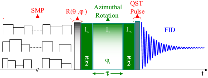
Figure 2: (Color online) The pulse sequence has four steps. In the first step the pseudo-NSCS $\left|I,I\right\rangle$ is implemented by the SMP technique. The second step consists of the non-selective pulses with parameters $\left(\theta,\varphi\right)$ that produce excited pseudo-NSCSs $\left|\zeta\left(\theta,\varphi\right)\right\rangle$. The third step is the azimuthal rotation through time $\tau$, which can be used to produce cyclic evolutions. The last step involves the read-out of the pseudo-NSCS (QST procedure).

IV.1 Initializing pseudo-NSCSs

To produce excited pseudo-NSCSs from $\left|I,I\right\rangle$, we apply non-selective pulses of strength $\omega_{1}$ and phase $\varphi_{s}$ during time interval $t=\theta/\omega_{1}$ (see Eq. (9)). As a first example, the excited pseudo-NSCS $\left|\zeta\left(\pi/2,0\right)\right\rangle=\left|-1\right\rangle$ can be generated by applying a non-selective $\pi/2$ pulse that produces a rotation about the negative $y$–axis. On the other hand, a rotation of $\pi/2$ about the positive $y$–axis of the vector state $\left|I,I\right\rangle$ generates the state $\left|\zeta\left(\pi/2,\pi\right)\right\rangle=\left|1\right\rangle$. We observe that the unitary transformation (of Eq. (9)) associated with non-selective pulses, acting on a given pseudo-NSCS, produces excited pseudo-NSCSs analogously to those discussed in Ref. duzzioni2007 .

In Fig. 3, we present experimental results for the deviation density matrix, in the form of bar charts of the real (left) and imaginary (middle) components, for the quantum states $\left|\zeta\left(0,\varphi\right)\right\rangle=\left|0\right\rangle$, $\left|\zeta\left(\pi/2,\pi\right)\right\rangle=\left|1\right\rangle$, $\left|\zeta\left(\pi/2,0\right)\right\rangle=\left|-1\right\rangle$,   $\left|\zeta\left(\pi/2,3\pi/2\right)\right\rangle=\left|i\right\rangle$,  $\left|\zeta\left(\pi/2,\pi/2\right)\right\rangle=\left|-i\right\rangle$, and $\left|\zeta\left(\pi,\varphi\right)\right\rangle=\left|\infty\right\rangle$ (see Tab. 1). The intensity of the elements of each deviation density matrix was obtained by QST. On the right of Fig. 3, the Husimi $\mathcal{Q}$-distribution was used to characterize these implemented quantum states, which is sketched on the Bloch sphere gordon1999 . The highest positive normalized intensity corresponds to the red color and the most negative intensity corresponds to the orange color. The highest intensity (red color) of the quasi-probability distribution function indicates the orientation of the spin nuclei magnetization. The large dispersion of the Husimi $\mathcal{Q}$-distribution function is due to the small spin value $I=3/2$, or analogously, the small number of particles $N=2I=3$ of an atomic system.

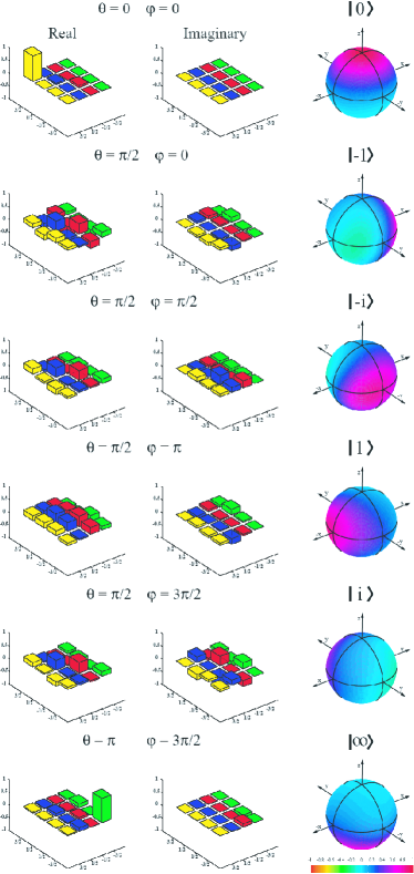
Figure 3: (Color online) Experimental results for the ²³Na nuclei in the sample of SDS. The QST results are represented by bar charts (left and middle column) for the implemented pseudo-NSCSs and on the Bloch Sphere (right column) by the Husimi $\mathcal{Q}$-distribution. The top bar chart represents the pseudo-NSCS $\left|0\right\rangle$, the left (right) bar chart showing the real (imaginary) part of the deviation density operator, and similarly for the other bar charts. The pseudo-NSCS $\left|0\right\rangle$ is implemented as explained in section IV by the SMP technique. The bottom bar chart shows the pseudo-NSCS $\left|\infty\right\rangle$, a state that is implemented by applying a rotation operator $\mathbf{R}_{\theta,\varphi}$ with $\theta=\pi$ and $\varphi=3\pi/2$ to the pseudo-NSCS $\left|0\right\rangle$. The pseudo-NSCS $\left|-1\right\rangle$ is implemented by applying a ${\pi}/{2}$ non-selective pulse in the negative $y-$direction to transform $\left|0\right\rangle$. Analogous remarks apply to the bar charts labeled as $\left|1\right\rangle$, $\left|i\right\rangle$, and $\left|-i\right\rangle$. In the right column, we present the calculated Husimi $\mathcal{Q}$-distribution of each deviation density matrix and, at the bottom, the intensity of the $\mathcal{Q}$–distribution function is encoded in the colour bar.

In order to compare the theoretical predictions with the experimental values of the deviation density matrices of Fig. 3, we present in Tab. 1 the complex phase $\zeta\left(\theta,\varphi\right)$ and the Bloch vector $\mathbf{n}$. The experimental values for $\theta$ and $\varphi$ were computed with Eqs. (3), (6), and (7).

		Theoretical		Experimental
$\theta$	$\varphi$	$\left|\zeta\left(\theta,\varphi\right)\right\rangle$	$\mathbf{n}$	$\left|\zeta\left(\theta,\varphi\right)\right\rangle$	$\mathbf{n}$
$0$	$0$	$\left|0\right\rangle$	$\left(0,0,1\right)$	$\left|0.02-0.01i\right\rangle$	$\left(-0.05,-0.02,0.99\right)$
$\frac{\pi}{2}$	$0$	$\left|-1\right\rangle$	$\left(1,0,0\right)$	$\left|-0.88-0.12i\right\rangle$	$\left(0.98,-0.14,0.12\right)$
$\frac{\pi}{2}$	$\frac{3\pi}{2}$	$\left|-i\right\rangle$	$\left(0,-1,0\right)$	$\left|-0.88i\right\rangle$	$\left(0,-0.99,0.13\right)$
$\frac{\pi}{2}$	$\pi$	$\left|1\right\rangle$	$\left(-1,0,0\right)$	$\left|0.79+0.25i\right\rangle$	$\left(-0.94,0.30,0.18\right)$
$\frac{\pi}{2}$	$\frac{\pi}{2}$	$\left|i\right\rangle$	$\left(0,1,0\right)$	$\left|-0.09+0.84i\right\rangle$	$\left(0.1,0.98,0.16\right)$
$\pi$	$0$	$\left|\infty\right\rangle$	$\left(0,0,-1\right)$	$\left|7.75+1.16i\right\rangle$	$\left(-0.25,0.04,-0.97\right)$

Table 1: Comparison between theoretical and experimental values obtained from the deviation density matrix of Fig. 3 by means of equations (3), (6) and (7). Experimental values are rounded to two decimal places.

IV.2 Controlling pseudo-NSCSs

Besides knowing how to initialize a quantum system, i.e., how to prepare the desired quantum state, an important task in quantum physics is the control of the quantum system with high accuracy. The implementation and control of pseudo-NSCSs are important for applications in quantum computing and geometric phases duzzioni2007 , squeezed states kitagawa1993 , and quantum metrology riedel2010 . In the present case, such control is performed through polar and azimuthal rotations.

Polar rotations – In the context of polar rotations, we have demonstrated the experimental control of angle $\theta$ by taking the initial quantum state $\left|\zeta\left(0,0\right)\right\rangle=\left|0\right\rangle$ and applying the rotation operator $\mathbf{R}_{\theta,\varphi}$, with  $\theta=0,\pi/18,2\pi/18,$ $\ldots,\pi$ (total of nineteen steps) and fixed $\varphi=\pi$. After each step, the state $\left|\zeta\left(\theta,\varphi\right)\right\rangle$ was reconstructed by QST (see pulse sequence in Fig. 2). First, the average values of the magnetic angular momenta $\left\langle\mathbf{I}_{x,y,z}\right\rangle$ were calculated for each deviation density matrix $\left|\zeta\left(\theta,\varphi\right)\right\rangle\left\langle\zeta\left(\theta,\varphi\right)\right|$. The experimental results (symbols) are shown in Fig. 4 together with the values obtained by numerical simulation (solid lines) and theoretical prediction (dashed lines). We use the term numerical simulation when we apply numerical recipes to the dynamics of evolution given by Hamiltonian (8), while the theoretical prediction is given by the evolution operator of Eq. (9). The differences between simulated data and theoretical prediction are caused by the quadratic term of Hamiltonian (8). Such a term is the main source of imperfections in the generation and control of the pseudo-NSCSs.

In order to find the fidelity of the experimental implementations, we compared the tomographed deviation density matrix $\rho_{Exp}$ with the theoretical prediction $\rho_{The}$, by calculating fortunato2002

$$F=\frac{{\mathtt{Tr}}\left\{\rho_{Exp}\cdot\rho_{The}\right\}}{\sqrt{{\mathtt{Tr}}\left\{\rho_{Exp}\cdot\rho_{Exp}\right\}{\mathtt{Tr}}\left\{\rho_{The}\cdot\rho_{The}\right\}}}\text{.}$$ (15)

The results for $F$ are presented in Fig. 4b and show that the experimental generation and control of the pseudo-NSCSs can be achieved with fidelity higher than 80 %.

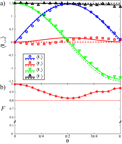
Figure 4: (Color online) Experimental results (symbols), numerical simulations (solid line), and theoretical predictions (dashed lines) of a polar rotation of the Bloch vector for the initial pseudo-NSCS $\left|0\right\rangle$, implemented experimentally by the SMP technique. QST is performed for nineteen different values of $\theta$ from 0 to $\pi$. The average values of the magnetic angular momentum components $\left\langle\mathbf{I}_{x,y,z}\right\rangle$ and the total angular momentum $\left\langle\mathbf{I}\right\rangle=\sqrt{\sum_{i=x,y,z}\left\langle\mathbf{I}_{i}\right\rangle^{2}}$ are shown in a). The accuracy of the polar rotations is calculated by the fidelity $F$ (Eq. (15)) between experimental results and theoretical prediction, as depicted in b).

Azimuthal rotations.– The azimuthal rotation is performed around the $z$-axis so that it can be achieved by the pulse sequence $\left[\pi/2\right]_{x}\rightarrow\left[\varphi_{\tau}\right]_{y}\rightarrow\left[\pi/2\right]_{-x}$, where the subscripts represent the phases of the non-selective pulses and the values in square brackets the rotation angles. This pulse sequence is referred to as composite pulse freeman1981 . As a first step in the experiment, we arbitrarily prepare the excited pseudo-NSCS $\left|\zeta\left(\pi/2,\pi\right)\right\rangle$. By applying the composite pulse sequence to the initial state $\left|\zeta\left(\pi/2,\pi\right)\right\rangle$ we can obtain thirty-three distinct pseudo-NSCSs $\left|\zeta\left(\pi/2,\pi+\varphi_{\tau}\right)\right\rangle$ with angular values $\varphi_{\tau}=0,\pi/16,2\pi/16,3\pi/16,\ldots,2\pi$ and $\theta$ fixed at $\pi/2$. Finally, the transformed state is reconstructed by the QST procedure.

The average values of magnetic angular momenta $\left\langle\mathbf{I}_{x,y,z}\right\rangle$  were  computed  for  each  deviation  density  matrix $\left|\zeta\left(\pi/2,\pi+\varphi_{\tau}\right)\right\rangle\left\langle\zeta\left(\pi/2,\pi+\varphi_{\tau}\right)\right|$. The experimental results (symbols) are plotted in Fig. 5a together with the values of the numerical simulation (solid lines) and theoretical prediction (dashed lines). As in the case of polar rotation, using one non–selective pulse, the differences between simulated data and theoretical prediction are caused by the quadratic term of Hamiltonian (8). However, in the study of azimuthal rotation we need four pulses: one to create the excited state $\left|\zeta\left(\pi/2,\pi\right)\right\rangle$ and three making up the composite pulse sequence. These additional pulses are another source of errors in the generation of the state, due to the error accumulated during the calibration of each pulse and time delays between them, which are of order 2–3 $\mu$s, despite being small, is not truly negligible. In the azimuthal rotation, the extra pulses and delays take 10–12 $\mu$s more time to implement than a polar rotation by the same angle. During this additional time, the contribution of the quadrupolar coupling is more evident, transforming the implemented pseudo-NSCS with a non-null degree of squeeze kitagawa1993 . This is the reason why the fidelity $F$ in Fig. 5b is, on average, lower than the fidelity in the polar case (see Fig. 4b). In order to diminish these errors it is necessary to calibrate non–selective pulses of short duration.

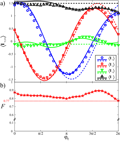
Figure 5: (Color online) Experimental results (symbols), numerical simulations (solid line), and theoretical predictions (dashed lines) of an azimuthal rotation of the Bloch vector for the initial pseudo-NSCS $\left|1\right\rangle$, implemented experimentally by the SMP technique. QST is performed for thirty-three different values of $\varphi_{\tau}$ from 0 to $2\pi$. The average values of the magnetic angular momentum components $\left\langle\mathbf{I}_{x,y,z}\right\rangle$ and the total angular momentum $\left\langle\mathbf{I}\right\rangle=\sqrt{\sum_{i=x,y,z}\left\langle\mathbf{I}_{i}\right\rangle^{2}}$ are shown in a). The accuracy of the azimuthal rotations is calculated by the fidelity $F$ (Eq. (15)) between experimental results and theoretical prediction as depicted in b).

V Theoretical application of the pseudo-NSCS

V.1 Geometric phase

In this section, we use the Mukunda-Simon formalism mukunda1993 to compute geometric phases that arise from the three distinct cyclic evolutions. For a system evolving according to the Schrödinger equation, the geometric phase $\phi_{G}$ can be defined as the difference between the total phase $\phi_{T}\left(\tau\right)=\arg\left[\left\langle\psi\left(0\right)|\psi\left(\tau\right)\right\rangle\right]$ and  the  dynamic  phase $\phi_{D}\left(\tau\right)=-i\int_{0}^{\tau}\left\langle\psi\left(t\right)\right|\frac{\partial}{\partial t}\left|\psi\left(t\right)\right\rangle$, i.e.,

$$\phi_{G}\left(\tau\right)=\arg\left[\left\langle\psi\left(0\right)|\psi\left(\tau\right)\right\rangle\right]+i\int_{0}^{\tau}\left\langle\psi\left(t\right)\right|\frac{\partial}{\partial t}\left|\psi\left(t\right)\right\rangle dt\text{,}$$ (16)

where $\tau$ is the overall time of the evolution duzzioni2007 ; duzzioni2005 ; fuentes2002 .

Before starting the calculation of the geometric phases, it is worth mentioning that this phase, acquired by the quadrupolar NMR system, is related only to the pseudo-pure state, since its definition (16) does not hold for general mixed states tong2004PRL . Assuming an initial pseudo-NSCS $\left|\zeta\left(\theta,\varphi\right)\right\rangle$, the geometric phase acquired by this quantum state is calculated while undergoing three distinct cyclic evolutions: $i)$ the free evolution under the NMR quadrupolar Hamiltonian (Eq. (8)), and the evolution of such a system under the analogous $ii)$ single- and $iii)$ two-mode BEC Hamiltonian. This analogy between the NMR quadrupolar system  and  BECs  was  explored  in Ref. auccaise2009 through the Holstein-Primakov formalism.

V.2 Free evolution of the NMR system

The first case to be analyzed is the free evolution of the quadrupolar system with the offset frequency set $\omega_{RF}=\omega_{L}-\omega_{Q}$. In this case the evolution operator, Eq. (12), is rewritten as

$$\mathcal{U}_{Ev}\left(\varphi^{\prime}\right)=\exp\left[-i\varphi^{\prime}\left(-\mathbf{I}_{z}+\frac{1}{6}\left(3\mathbf{I}_{z}^{2}-\mathbf{I}^{2}\right)\right)\right]\text{,}$$ (17)

where $\varphi^{\prime}=\omega_{Q}t$, which from now on will vary from $0$ to $2\pi$. Using Eq. (16) and computing the average values of operators $\mathbf{I}_{z}$ and $\mathbf{I}$ for the pseudo-NSCS $\left|\zeta\left(\theta,\varphi\right)\right\rangle$, the geometric phase can be expressed by:

$${}^{A}\phi_{G}\left(\mathcal{C}\right)=\pi I\left[\left(\left(I-\frac{1}{2}\right)\cos^{2}\theta-2\cos\theta+\frac{5}{2}-I\right)\right]\text{.}$$ (18)

This expression has a quadratic dependence on the harmonic function, because the Hamiltonian in this analysis is quadratic in the nuclear spin angular momentum operator. Applying Eq. (18) to a spin $I=1/2$ nucleus, we find

$${}^{A}\phi_{G}\left(\mathcal{C}\right)=\pi\left(1-\cos\theta\right)\text{,}$$ (19)

which corroborates the well known results reported for two-level particles in references jones2000 ; ekert2000 ; leek2007 ; shapere . Note that in this case the single harmonic function arises from the linear dependence of the nuclear spin angular momentum operator in the Hamiltonian, which allows the connection between the geometric phase and half of the solid angle on the Bloch sphere. On the other hand, for spin $I=3/2$, the presence of the quadrupolar term makes the geometric phase proportional to the square of the solid angle.

V.3 NMR system evolving as a single-mode BEC

As a second example of the free evolution of the NMR quadrupolar system, we explore its analogy with the single-mode BEC, as reported in Ref. auccaise2009 . In this description, the frequency $\omega_{RF}$ of the evolution operator in Eq. (12) satisfies the mathematical expression $2I-1=\frac{2\left(\omega_{L}-\omega_{RF}\right)}{\omega_{Q}}$ (see Eq. (7) of Ref. auccaise2009 ). Then $\mathcal{U}_{Ev}\left(\varphi^{\prime}\right)$ is written:

$$\mathcal{U}_{Ev}\left(\varphi^{\prime}\right)=\exp\left[-i\frac{\varphi^{\prime}}{2}\left(\mathbf{I}_{z}^{2}-\left(2I-1\right)\mathbf{I}_{z}-\frac{I^{2}+I}{3}\mathbf{1}\right)\right]\text{,}$$ (20)

where the angular parameter is denoted by $\varphi^{\prime}=\omega_{Q}t$. The geometric phase acquired by the pseudo-NSCS $\left|\zeta\left(\theta,\varphi\right)\right\rangle$ transformed by the operator (20) is

$${}^{B}\phi_{G}\left(\mathcal{C}\right)=\frac{\pi I\left(2I-1\right)}{2}\left(3+\cos\theta\right)\left(1-\cos\theta\right)\text{.}$$ (21)

In this interpretation, the geometric phase displays a qua-dra-tic dependence on the harmonic function, which is linked to the quadratic dependence of the number operator in the Holstein-Primakov representation mead1983 . We note that for $I=1/2$ the geometric phase is null. This is consistent with a discussion on geometric phase in a study of the quasiparticle dynamics in a BEC where one particle becomes a free particle and is not part of the condensate zhang2006PRL .

V.4 NMR system evolving as a two-mode BEC

In the third case, the two-mode BEC Hamiltonian in the Schwinger representation (see Eq. (14) of Ref. chen2004 ) is simulated by Hamiltonian (8) of the NMR system. In this  description, the  pseudo-angular  momentum  operators $\left(\mathbf{J}_{i=x,y,z}\right)$ are mapped on to the nuclear spin momentum operators $\left(\mathbf{I}_{i=x,y,z}\right)$, and the Hamiltonian parameters are mapped by $\omega_{0}\rightarrow\left(\omega_{RF}-\omega_{L}\right)$, $q\rightarrow\omega_{Q}/2$, $G\rightarrow\omega_{1}$ and $\varphi\rightarrow\varphi_{s}$. We will work in a particular configuration where the scattering lengths satisfy the relation $A_{a}:A_{ab}:A_{b}=1.03:1:0.97$ for modes $a$ and $b$ of the BEC duzzioni2007 , implying $q=0$. This is usually achieved through Feshbach resonances, as discussed in references leggett2001 ; duzzioni2007 ; fuentes2002 ; chen2004 . We also impose the condition that the external laser field coupling the two modes is turned off ($G=0$). The net atomic evolution is a rotation around the $z$–axis of frequency $\omega_{0}$, which one in the NMR scenario is implemented by means of the composite pulse sequence explained in section IV, i.e.

$$\mathcal{U}\left(\varphi^{\prime}\right)=\left[\frac{\pi}{2}\right]_{x}\longrightarrow\left[\varphi^{\prime}\right]_{y}\longrightarrow\left[\frac{\pi}{2}\right]_{-x}\text{,}$$

where the pulse sequence is read from left to right. After a cyclic evolution of state $\left|\zeta\left(\theta,\varphi\right)\right\rangle$, the geometric phase is:

$${}^{C}\phi_{G}\left(\mathcal{C}\right)=-2\pi I\left(1-\cos\theta\right)\text{,}$$ (22)

reproducing a similar mathematical expression in Eq. (14) of Ref. fuentes2002 for an adiabatic evolution. In this case the geometric phase displays a linear dependence on the harmonic function, which reflects the linear dependence of the Hamiltonian in the nuclear spin angular momentum operator.

As in the Section V.2, the particular case of the geometric phase for a nuclear spin $I=1/2$ gives:

$${}^{C}\phi_{G}\left(\mathcal{C}\right)=-\pi\left(1-\cos\theta\right)\text{,}$$

a result that resembles the previous expression (19) for a spin $I=1/2$ particle. The negative sign means the opposite direction to the nuclear spin rotation. Indeed, this is due to the equivalence between superposition of spin $\left|\uparrow\right\rangle$ and spin $\left|\downarrow\right\rangle$ and the ACS definition for a two level-system.

VI Conclusion

In this paper we have described how it is possible to transfer the ACS concepts to the nuclear quadrupolar system labeled as a pseudo-NSCS. We experimentally showed how to initialize and to tomograph the pseudo-NSCS. The experimental manipulation of this state was performed by polar and azimuthal rotations, in which we note that the greatest obstacle to perfect initialization and control is the quadrupolar term of the NMR Hamiltonian. We also studied theoretically the geometric phase generated by the evolution of the pseudo-NSCS in three cases: $i)$ free evolution of the NMR system, $ii)$ single and $iii)$ two mode BEC. In the first and second cases, the geometric phase is a quadratic function of $\cos\theta$ for $I>1/2$, which is a signature of the quadrupolar term. For $I=1/2$, the geometric phase is $\pi(1-\cos\theta)$ for free evolution of the NMR system and null for the single mode BEC case. In the latter case, for $\theta>0$, the null geometric phase indicates there is no condensation. In the third case, the geometric phase acquired by the pseudo-NSCS under the action of a composite pulse sequence reproduces the same result as a geometric phase generated by a cyclic azimuthal rotation. The present study would be still more complete if one could measure experimentally the geometric phase discussed in each case. This task could be undertaken with two coupled nuclear spin systems, one spin $I>1/2$ and the other $S\geq 1/2$ (by analogy to Ref. jones2000 ), which we will try to implement in the near future. Finally, the concept of pseudo–NSCS in the NMR quadrupolar scenario offers new insights into spin squeezed states and quantum metrology implemented in liquid crystals or solid matter.

- (1) Roy J. Glauber, Phys. Rev., 130, 2529–2539, (1963).
- (2) F. T. Arecchi, Eric Courtens, Robert Gilmore and Harry Thomas, Phys. Rev. A, 6, 2211–2237, (1972).
- (3) A. Perelomov, Generalized Coherent States and Their Applications, Text and Monographs in Physics - Springer-Verlag, (1985).
- (4) J. M. Raimond, M. Brune and S. Haroche, Rev. Mod. Phys., 73, 565–582, (2001).
- (5) D. Leibfried, R. Blatt, C. Monroe and D. Wineland, Rev. Mod. Phys., 75, 281–324, (2003).
- (6) Anthony J. Leggett, Rev. Mod. Phys., 73, 307–356, (2001).
- (7) Z.-D. Chen, J.-Q. Liang, S.-Q. Shen and W.-F. Xie, Phys. Rev. A, 69, 023611, (2004).
- (8) D. Gordon and C. M. Savage, Phys. Rev. A, 59, 4623–4629, (1999).
- (9) Nir Bar-Gill, Gershon Kurizki, Markus Oberthaler and Nir Davidson, Phys. Rev. A, 80, 053613, (2009).
- (10) Julian Grond, Gregory von Winckel, Jörg Schmiedmayer and Ulrich Hohenester, Phys. Rev. A, 80, 053625, (2009).
- (11) Jonathan A. Jones, Vlatko Vedral, Artur Ekert and Giuseppe Castagnoli, Nature, 403, 6772, (2000).
- (12) H. Chen, M. Hu, J. Chen and J. Du, Phys. Rev. A, 80, 054101, (2009).
- (13) Yukihiro Ota and Yasushi Kondo, Phys. Rev. A, 80, 024302, (2009).
- (14) C. W. Niu, G. F. Xu, Longjiang Liu, L. Kang, D. M. Tong and L. C. Kwek, Phys. Rev. A, 81, 012116, (2010).
- (15) M. V. Berry, Proc. R. Soc. Lond. A, 392, 45–57, (1984).
- (16) Akira Tomita and Raymond Y. Chiao, Phys. Rev. Lett., 57, 937–940, (1986).
- (17) Rajendra Bhandari and Joseph Samuel, Phys. Rev. Lett., 60, 1211–1213, (1988).
- (18) P. J. Leek, J. M. Fink, A. Blais, R. Bianchetti, M. Goppl, J. M. Gambetta, D. I. Schuster, L. Frunzio, R. J. Schoelkopf and A. Wallraff, Science, 318, 1889-1892, (2007).
- (19) N. Mukunda and R. Simon, Annals of Physics, 228, 205 - 268, (1993).
- (20) Z. S. Wang, G. Q. Liu and Y. H. Ji, Phys. Rev. A, 79, 054301, (2009).
- (21) F. O. Prado, E. I. Duzzioni, M. H. Y. Moussa, N. G. de Almeida and C. J. Villas-Boas, Phys. Rev. Lett., 102, 073008, (2009).
- (22) E. I. Duzzioni, L. Sanz, S. S. Mizrahi and M. H. Y. Moussa, Phys. Rev. A, 75, 032113, (2007).
- (23) Jonas Larson and Erik Sjoqvist, Phys. Rev. A, 79, 043627, (2009).
- (24) D. Suter, Gerard C. Chingas, Robert A. Harris and A. Pines, Molecular Physics, 61, 1327–1340, (1987).
- (25) A. Ekert, M. Ericsson, P. Hayden, H. Inamori, J. A. Jones, Daniel K. L. Oi and V. Vedral, Journal of Modern Optics, 47, 2501–2513, (2000).
- (26) Wang Xiang-Bin and Matsumoto Keiji, Phys. Rev. Lett., 87, 097901, (2001).
- (27) Shi-Liang Zhu and Z. D. Wang,, Phys. Rev. Lett., 89, 097902, (2002).
- (28) Shi-Liang Zhu and Z. D. Wang, Phys. Rev. A, 66, 042322, (2002).
- (29) A. Abragam, Principles of Nuclear Magnetism, Oxford Science Publications, Reprinted, A Editora,Cidade Tal, (1994).
- (30) R. Auccaise, J. Teles, T. J. Bonagamba, I. S. Oliveira, E. R. deAzevedo and R. S. Sarthour, The Journal of Chemical Physics, 130, 144501, (2009).
- (31) G. J. Milburn, J. Corney, E. M.Wright and D. F. Walls, Phys. Rev. A, 55, 4318–4324, (1997).
- (32) Chuanwei Zhang, Artem M. Dudarev and Qian Niu, Phys. Rev. Lett., 97, 040401, (2006).
- (33) A. Inomata, H. Kuratsuji and C. C. Gerry, Path integrals and coherent states of SU(2) and SU(1,1), World Scientific, First Edition, (1992).
- (34) I. S. Oliveira, T. J. Bonagamba, R. S. Sarthour, J. C. C. Freitas, and E. R. de Azevedo, NMR Quantum Information Processing, Elsevier - Amsterdan (2007).
- (35) Masahiro Kitagawa and Masahito Ueda, Phys. Rev. A, 47, 5138–5143, (1993).
- (36) E. M. Fortunato, M. A. Pravia, N. Boulant, G. Teklemariam, Timothy F. Havel and David G. Cory, The Journal of Chemical Physics, 116, 7599–7606, (2002).
- (37) J. Teles, E. R. deAzevedo, R. Auccaise, R. S. Sarthour, I. S. Oliveira and T. J. Bonagamba, The Journal of Chemical Physics, 126, 154506, (2007).
- (38) Riedel, Max F. and Böhi, Pascal and Li, Yun and Hänsch, Theodor W. and Sinatra, Alice and Treutlein, Philipp, Nature, 464, 1170–1173, (2010).
- (39) Ray Freeman, Thomas A. Frenkiel and Malcolm H. Levitt, Journal of Magnetic Resonance (1969), 44, 409 - 412, (1981).
- (40) E. I. Duzzioni, C. J. Villas-Boas, S. S. Mizrahi, M. H. Y. Moussa and R. M. Serra, EPL (Europhysics Letters), 72, 21-27, (2005).
- (41) I. Fuentes-Guridi, J. Pachos, S. Bose, V. Vedral and S. Choi, Phys. Rev. A, 66, 022102, (2002).
- (42) D. M. Tong, E. Sj qvist, L. C. Kwek, and C. H. Oh, Phys. Rev. Lett., 93, 080405 (2004).
- (43) Alfred Shapere and Frank Wilczek, Geometric Phases in Physics, World Scientific Publishing Co. Pte. Ltd, Advanced Series in Mathematical Physics Vol 5, First Edition, 1989.
- (44) L.R. Mead and and N. Papanicolaou, Phys. Rev. B, 28, 1633 (1983).