Polyakov loop analysis with Dirac-mode expansion

Abstract:

In order to investigate the direct relation between confinement and chiral symmetry breaking in QCD, we investigate the Polyakov loop in terms of the Dirac eigenmodes in both confined and deconfined phases. Using the Dirac-mode expansion method in SU(3) lattice QCD, we analyze the contribution of low-lying and higher Dirac-modes to the Polyakov loop, respectively. In the confined phase below $T_{c}$, after removing low-lying Dirac-modes, the chiral condensate $\langle\bar{q}q\rangle$ is largely reduced, however, the Polyakov loop remains almost zero and $Z_{3}$-center symmetry is unbroken. These results indicate that the system is still in the confined phase without low-lying Dirac-modes. By higher Dirac-modes cut, the Polyakov loop also remains almost zero below $T_{c}$. We also analyze the Polyakov loop in the deconfined phase above $T_{c}$. We find that the Polyakov loop and $Z_{3}$-symmetry behavior are insensitive to low-lying and higher Dirac-modes in both confined and deconfined phases.

1 Introduction

Quantum chromodynamics (QCD) is the fundamental theory of the strong interaction, however, its non-perturbative properties such as confinement and chiral symmetry breaking are not yet well understood. In particular, to clarify the correspondence between confinement and chiral symmetry breaking is one of difficult and interesting subjects [1, 2, 3, 4, 5, 6, 7]. As an evidence of the close relation between them, lattice QCD calculation shows that simultaneous deconfinement and chiral phase transition at finite temperature [8].

As shown in the Banks-Casher relation [9], the chiral condensate $\langle\bar{q}q\rangle$ is proportional to the Dirac zero-mode density as

$$\langle\bar{q}q\rangle=-\lim_{m\rightarrow 0}\lim_{V\rightarrow\infty}\pi\langle\rho(0)\rangle,$$ (1)

where $\rho(\lambda)$ is the Dirac spectral density. Thus, the low-lying Dirac eigenmodes directly relate to chiral symmetry breaking, however, their relation to confinement is still unclear.

Therefore, it is interesting to analyze confinement in terms of the relevant degrees of freedom for chiral symmetry breaking, i.e., the low-lying Dirac eigenmodes. For example, based on the Gattringer’s formula [1], the Polyakov loop can be investigated by the sum of Dirac spectra with twisted boundary condition on lattice [2, 3, 4]. In our previous studies [5, 6], we formulated the Dirac-mode expansion method in lattice QCD, and investigated the Dirac-mode dependence of the Wilson loop and the interquark potential. It is also reported that hadrons still exist as bound states without “chiral symmetry breaking” by removing low-lying Dirac-modes [10, 11].

In this paper, we investigate the Dirac-mode dependence of the Polyakov loop in both confined and deconfined phases at finite temperature, using Dirac-mode expansion method in lattice QCD [5, 6, 7]. In Sec. 2, we review the Dirac-mode expansion method, and formulate the Dirac-mode projected Polyakov loop. In Sec. 3, we perform the lattice QCD calculations for the Polyakov loop with Dirac-mode projection. Section 4 is devoted for the summary.

2 Dirac-mode expansion method in lattice QCD

Here, we introduce the Dirac-mode expansion technique in lattice QCD [5, 6, 7], and formulation of the Dirac-mode projected Polyakov loop.

2.1 Dirac-mode expansion in lattice QCD

Using the link-variable $U_{\mu}\in\mathrm{SU}(N_{c})$, the Dirac operator ${\ooalign{\hfil/\hfil\crcr$D$}}=\gamma_{\mu}D_{\mu}$ is given by

$${\ooalign{\hfil/\hfil\crcr$D$}}_{x,y}\equiv\frac{1}{2a}\sum_{\mu=1}^{4}\gamma_{\mu}\left[U_{\mu}(x)\delta_{x+\hat{\mu},y}-U_{-\mu}(x)\delta_{x-\hat{\mu},y}\right],$$ (2)

with a lattice spacing $a$, and $U_{-\mu}(x)\equiv U_{\mu}^{\dagger}(x-\hat{\mu})$. Here, $\gamma$-matrix is defined to be hermitian, i.e., $\gamma_{\mu}^{\dagger}=\gamma_{\mu}$. Thus, / $D$ becomes an antihermitian operator, and Dirac eigenvalues are pure imaginary. We introduce the normalized Dirac eigenstate $|n\rangle$, which satisfies

$${\ooalign{\hfil/\hfil\crcr$D$}}|n\rangle=i\lambda_{n}|n\rangle,$$ (3)

with $\lambda_{n}\in\mathbf{R}$, and an eigenfunction $\psi_{n}(x)$ is expressed as

$$\psi_{n}(x)\equiv\langle x|n\rangle,$$ (4)

which satisfies ${\ooalign{\hfil/\hfil\crcr$D$}}\psi_{n}=i\lambda_{n}\psi_{n}$.

We introduce the operator formalism in lattice QCD [5, 6, 7], which is constructed from the link-variable operator $\hat{U}_{\mu}$. The link-variable operator is defined by the matrix element as

$$\langle x|\hat{U}_{\mu}|y\rangle=U_{\mu}(x)\delta_{x+\hat{\mu},y},$$ (5)

using the original link-variable $U_{\mu}(x)$. We define the Dirac-mode matrix element $\langle n|\hat{U}_{\mu}|m\rangle$ as

$$\langle n|\hat{U}_{\mu}|m\rangle = \sum_{x}\langle n|x\rangle\langle x|\hat{U}_{\mu}|x+\hat{\mu}\rangle\langle x+\hat{\mu}|m\rangle=\sum_{x}\psi_{n}^{\dagger}(x)U_{\mu}(x)\psi_{m}(x+\hat{\mu}),$$ (6)

with the Dirac eigenfunction $\psi_{n}(x)$.

Considering the completeness relation $\sum_{n}|n\rangle\langle n|=1$, any operator $\hat{O}$ can be expressed as

$$\hat{O}=\sum_{n}\sum_{m}|n\rangle\langle n|\hat{O}|m\rangle\langle m|,$$ (7)

using the Dirac-mode basis. Note that this procedure is just the insertion of unity, and it is mathematically correct. This expansion (7) is the mathematical basis of the Dirac-mode expansion method [5, 6, 7]. Next, we consider the Dirac-mode projection by introducing projection operator as

$$\hat{P}\equiv\sum_{n\in\mathcal{A}}|n\rangle\langle n|,$$ (8)

for arbitrary set $\mathcal{A}$ of eigenmodes. For example, IR and UV mode-cut operators are given by

$$\hat{P}_{\rm IR}\equiv\sum_{|\lambda_{n}|\geq\Lambda_{\rm IR}}|n\rangle\langle n|,\qquad\hat{P}_{\rm UV}\equiv\sum_{|\lambda_{n}|\leq\Lambda_{\rm UV}}|n\rangle\langle n|,$$ (9)

with the IR/UV cutoff scale $\Lambda_{\rm IR}$ and $\Lambda_{\rm UV}$.

Using the projection operator $\hat{P}$, the Dirac-mode projected link-variable operator is given by

$$\hat{U}_{\mu}^{P}\equiv\hat{P}\hat{U}_{\mu}\hat{P}=\sum_{n\in\mathcal{A}}\sum_{m\in\mathcal{A}}|n\rangle\langle n|\hat{U}_{\mu}|m\rangle\langle m|.$$ (10)

We can investigate the Dirac-mode dependence of various kinds of quantities, e.g., the Wilson loop [5, 6], using the projected link-variable $\hat{U}_{\mu}^{P}$ instead of the original link-variable operator $\hat{U}_{\mu}$.

2.2 Polyakov loop operator and Dirac-mode projection

Next, we formulate the Dirac-mode projected Polyakov loop. Here, we consider the periodic SU(3) lattice with the space-time volume $V=L^{3}\times N_{t}$ and the lattice spacing $a$. In the operator formalism of lattice QCD, the Polyakov loop operator is given by

$$\hat{L}_{P}\equiv\frac{1}{3V}\prod_{i=1}^{N_{t}}\hat{U}_{4}=\frac{1}{3V}\hat{U}_{4}^{N_{t}}$$ (11)

with the temporal link-variable operator $\hat{U}_{4}$. By the functional trace “Tr”, the Polyakov loop operator coincides with the standard definition as

$$\mathrm{Tr}\ \hat{L}_{P} = \frac{1}{3V}\mathrm{Tr}\ \large\{\prod_{i=1}^{N_{t}}\hat{U}_{4}\large\}=\frac{1}{3V}\mathrm{tr}\sum_{\vec{x},t}\langle\vec{x},t|\prod_{i=1}^{N_{t}}\hat{U}_{4}|\vec{x},t\rangle$$ (12)

$$= \frac{1}{3V}\mathrm{tr}\sum_{\vec{x},t}\langle\vec{x},t|\hat{U}_{4}|\vec{x},t+a\rangle\langle\vec{x},t+a|\hat{U}_{4}|\vec{x},t+2a\rangle\cdots\langle\vec{x},t+(N_{t}-1)a|\hat{U}_{4}|\vec{x},t\rangle$$

$$= \frac{1}{3V}\mathrm{tr}\sum_{\vec{x},t}U_{4}(\vec{x},t)U_{4}(\vec{x},t+a)\cdots U_{4}(\vec{x},t+(N_{t}-1)a)=\langle L_{P}\rangle,$$

where “tr” denotes the trace over SU(3) color index.

We define the Dirac-mode projected Polyakov loop $\langle L_{P}^{\rm proj.}\rangle$ as

$$L_{P}^{\rm proj.} \equiv \frac{1}{3V}\mathrm{Tr}\ \large\{\prod_{i=1}^{N_{t}}\hat{U}_{4}^{P}\large\}=\frac{1}{3V}\mathrm{Tr}\left\{\hat{P}\hat{U}_{4}\hat{P}\hat{U}_{4}\hat{P}\cdots\hat{P}\hat{U}_{4}\hat{P}\right\}$$ (13)

$$= \frac{1}{3V}\mathrm{tr}\sum_{n_{1},n_{2},\dots,n_{N_{t}}\in\mathcal{A}}\langle n_{1}|\hat{U}_{4}|n_{2}\rangle\langle n_{2}|\hat{U}_{4}|n_{3}\rangle\cdots\langle n_{N_{t}}|\hat{U}_{4}|n_{1}\rangle.$$

In particular, the IR and the UV Dirac-mode projected Polyakov loop are denoted as

$$\langle L_{P}\rangle_{\rm IR} \equiv \frac{1}{3V}\mathrm{tr}\sum_{|\lambda_{n_{i}}|\geq\Lambda_{\rm IR}}\langle n_{1}|\hat{U}_{4}|n_{2}\rangle\cdots\langle n_{N_{t}}|\hat{U}_{4}|n_{1}\rangle,$$ (14)

$$\langle L_{P}\rangle_{\rm UV} \equiv \frac{1}{3V}\mathrm{tr}\sum_{|\lambda_{n_{i}}|\leq\Lambda_{\rm UV}}\langle n_{1}|\hat{U}_{4}|n_{2}\rangle\cdots\langle n_{N_{t}}|\hat{U}_{4}|n_{1}\rangle,$$ (15)

with the IR/UV eigenvalue cutoff $\Lambda_{\rm IR}$ and $\Lambda_{\rm UV}$.

3 Lattice QCD calculation for Dirac-mode projected Polyakov loop

In this section, we calculate the Dirac-mode projected Polyakov loop using SU(3) lattice QCD at the quenched level. We evaluate the full Dirac eigenmodes using LAPACK [12]. For actual calculation, we use the eigenmode basis of the Kogut-Susskind (KS) operator of

$$D_{x,y}^{\rm KS}\equiv\frac{1}{2a}\sum_{\mu=1}^{4}\eta_{\mu}(x)\left[U_{\mu}(x)\delta_{x+\hat{\mu},y}-U_{-\mu}(x)\delta_{x-\hat{\mu},y}\right],$$ (16)

with $\eta_{1}(x)\equiv 1$ and $\eta_{\mu}(x)\equiv(-1)^{x_{1}+\cdots+x_{\mu-1}}$ ($\mu\geq 2$) in order to reduce the computational cost. The use of the KS-Dirac operator gives the same result as the original Dirac operator in Eq. (2) for the Polyakov loop.

3.1 The confined phase

First, we analyze the Polyakov loop in the confined phase below $T_{c}$. Here, we use $6^{4}$ lattice with $\beta=5.6$, which corresponds to the lattice spacing $a\simeq 0.25$ fm and $T\equiv 1/(N_{t}a)\simeq 0.13$ GeV [5, 6, 7].

Figure 1 shows the lattice QCD results for the Dirac spectral density $\rho(\lambda)$, and IR/UV-cut spectral density $\rho_{\rm IR}(\lambda)\equiv\rho(\lambda)\theta(|\lambda|-\Lambda_{\rm IR})$, $\rho_{\rm UV}(\lambda)\equiv\rho(\lambda)\theta(\Lambda_{\rm UV}-|\lambda|)$ with $\Lambda_{\rm IR}=0.5a^{-1}$ and $\Lambda_{\rm UV}=2.0a^{-1}$. The total number of the KS Dirac-mode is $L^{3}\times N_{t}\times 3=3888$, and both mode cuts correspond to removing about 400 modes.

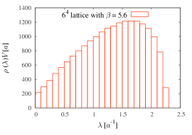
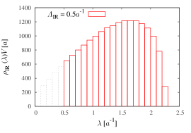
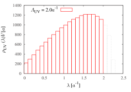
Figure 1: The spectral density $\rho(\lambda)$ of the Dirac operator on $6^{4}$ lattice with $\beta=5.6$, i.e., $a=0.25$ fm: (a) original spectral density, (b) IR-cut $\rho_{\rm IR}(\lambda)$ at $\Lambda_{\rm IR}=0.5a^{-1}$, (c) UV-cut $\rho_{\rm UV}(\lambda)$ at $\Lambda_{\rm UV}=2.0a^{-1}$.

Figure 2 shows the scatter plot of the original Polyakov loop, low-lying Dirac-modes cut at $\Lambda_{\rm IR}=0.5a^{-1}$, and the higher Dirac-modes cut at $\Lambda_{\rm UV}=2.0a^{-1}$, respectively. As shown in Fig. 2(a), the Polyakov loop is almost zero, i.e., $\langle L_{P}\rangle\simeq 0$, which indicates the confined phase.

Then, we consider low-lying Dirac-modes projection, which leads to the effective restoration of chiral symmetry breaking [6, 9, 10, 11]. In the presence of the IR cut $\Lambda_{\rm IR}$, the quark condensate is given by

$$\langle\bar{q}q\rangle_{\rm IR}=-\frac{1}{V}\sum_{\lambda_{n}\geq\Lambda_{\rm IR}}\frac{2m}{\lambda_{n}^{2}+m^{2}}.$$ (17)

At the IR cut parameter $\Lambda_{\rm IR}=0.5a^{-1}\simeq 0.4$ GeV, only 2% of the quark condensate remains as $\langle\bar{q}q\rangle_{\rm IR}/\langle\bar{q}q\rangle\simeq 0.02$ around the physical region $m\simeq 5$ MeV [6]. However, as shown in Fig. 2(b), the Polyakov loop $\langle L_{P}\rangle_{\rm IR}$ remains almost zero and $Z_{3}$-center symmetry is unbroken, and these facts indicate that the system still remains in the confined phase, even without chiral symmetry breaking.

In addition to the low-lying mode cut, we show the higher Dirac-modes cut in Fig. 2(c). In this case, the chiral condensation is almost unchanged, and the Polyakov loop remains almost zero. Therefore, the Polyakov loop is insensitive to both low-lying and higher Dirac eigenmodes.

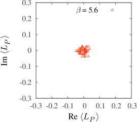
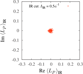
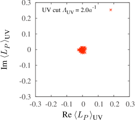
Figure 2: The scatter plot of the Polyakov loop in the confined phase on $6^{4}$ lattice with $\beta=5.6$, i.e., $a=0.25$ fm and $T\equiv 1/(N_{t}a)\simeq 0.2$ GeV. (a) The original (no Dirac-mode cut) Polyakov loop. (b) The low-lying Dirac-mode cut at $\Lambda_{\rm IR}=0.5a^{-1}$. (c) The higher Dirac-mode cut at $\Lambda_{\rm UV}=2.0a^{-1}$.

3.2 The deconfined phase at high temperature

Next, we investigate the Polyakov loop in the deconfined phase at high temperature. Here, we use $6^{3}\times 4$ lattice with $\beta=6.0$, which corresponds to $a=0.10$ fm and $T\equiv 1/(N_{t}a)\simeq 0.5$ GeV. The total number of the KS Dirac-mode is $L^{3}\times N_{t}\times 3=2592$.

We show the original Polyakov loop, typical low-lying mode cut at $\Lambda_{\rm IR}=0.5a^{-1}$, and higher mode cut at $\Lambda_{\rm UV}=2.0a^{-1}$ in Fig. 3. These mode cuts correspond to removing about 200 eigenmodes. As shown in Fig. 3(a), the Polyakov loop has non-zero expectation value $\langle L_{P}\rangle\neq 0$, and shows the center group $Z_{3}$ structure on the complex plane. These behaviors indicate the deconfined phase.

As shown in Figs. 3(b) and (c), the Polyakov loop shows the characteristic behaviors in the deconfined phase even after removing low-lying or higher Dirac-modes. To be strict, the UV-cut Polyakov loop has a smaller absolute value than the IR-cut Polyakov loop, although the number of UV-cut modes is comparable to that of the IR-cut case. This suggests that contributions of the higher Dirac-modes are much larger than low-lying modes [2]. However, apart from the normalization, both IR and UV cut Polyakov loops show the characteristic $Z_{3}$-pattern in the deconfined phase, and hence these Dirac-modes seem to be insensitive to the Polyakov loop properties.

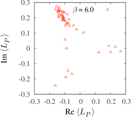
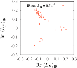
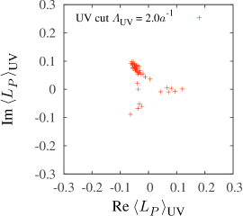
Figure 3: The scatter plot of the Polyakov loop in the deconfined phase on $6^{3}\times 4$ lattice with $\beta=6.0$, i.e., $a=0.10$ fm and $T\equiv 1/(N_{t}a)\simeq 0.5$ GeV. (a) The original (no Dirac-mode cut) Polyakov loop. (b) The low-lying Dirac-mode cut at $\Lambda_{\rm IR}=0.5a^{-1}$. (c) The higher Dirac-mode cut at $\Lambda_{\rm UV}=2.0a^{-1}$.

Figure 4 shows the Dirac spectral densities in confined and deconfined phases on $6^{3}\times 4$ lattice with $\beta=5.6$ and $6.0$, respectively. We also compare their low-lying spectral densities in Fig. 4(c). In the deconfinement phase, the low-lying Dirac-modes are suppressed, which leads to the chiral restoration. The chiral condensate is also reduced by the IR cut of the Dirac-modes as in Eq. (17). On the other hand, there seems no clear correspondence between the Dirac spectral densities and the Polyakov loop.

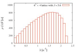
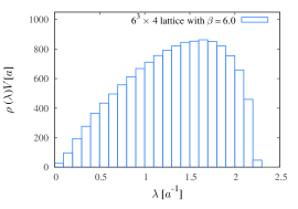
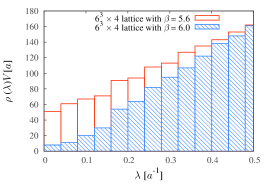
Figure 4: The Dirac spectral densities in confined and deconfined phases, respectively (a) $6^{3}\times 4$ lattice with $\beta=5.6$ in the confined phase. (b) $6^{3}\times 4$ lattice with $\beta=6.0$ in the deconfined phase. (c) The comparison between confined and deconfined phases on low-lying spectral densities.

3.3 $\beta$-dependence of the Dirac-mode projected Polyakov loop

Finally, we investigate $\beta$-dependence of the Dirac-mode projected Polyakov loop. Here, we adopt $6^{3}\times 4$ lattice with $\beta=5.4\sim 6.0$.

Figure 5 is the absolute values of the Polyakov loop with typical Dirac-mode projections, and the original Polyakov loop data are also added for comparison. In this lattice volume, the deconfinement phase transition occurs around $\beta=5.6\sim 5.7$. As shown in Fig. 5, both low-lying and higher Dirac-mode projected Polyakov loops show the similar $\beta$-dependence as the original data, apart from a normalization factor. This Dirac-mode insensitivity of the Polyakov loop is consistent with the results in the previous subsections.

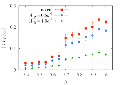
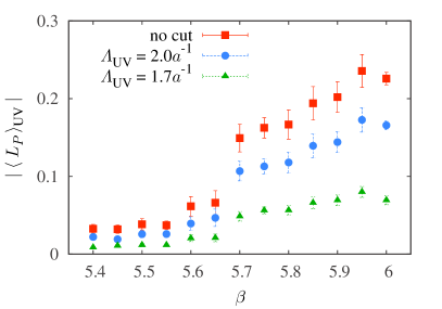
Figure 5: $\beta$-dependence of the absolute value of the Polyakov loop on $6^{3}\times 4$ lattice. (a) The IR Dirac-mode cut with $\Lambda_{\rm IR}=0.5a^{-1}$ and $1.0a^{-1}$. (b) The UV Dirac-mode cut with $\Lambda_{\rm UV}=2.0a^{-1}$ and $1.7a^{-1}$.

4 Summary

In this paper, we have analyzed the Polyakov loop in terms of the Dirac eigenmodes using SU(3) lattice QCD. We have carefully removed relevant degrees of freedom for chiral symmetry breaking from the Polyakov loop.

In the confined phase below $T_{c}$, the Polyakov loop is almost zero, i.e., $\langle L_{P}\rangle\simeq 0$. By removing low-lying Dirac-modes, the chiral condensate $\langle\bar{q}q\rangle$ is largely reduced. However, we have found that the Polyakov loop remains almost zero as $\langle L_{P}\rangle_{\rm IR}\simeq 0$ even without low-lying Dirac-modes, and this fact indicates that the system still remains in the confined phase. We have also investigated contributions from higher Dirac-modes to the Polyakov loop, and have found no change of the Polyakov loop without higher Dirac-modes. Therefore, there seems no specific region of the Dirac eigenmodes essential for the Polyakov loop.

We have also investigated the Polyakov loop in the deconfined phase at high temperature. In the deconfined phase, the Polyakov loop has non-zero expectation value, i.e., $\langle L_{P}\rangle\neq 0$, which distributes around $Z_{3}$ elements in the complex plane. These characteristic behaviors also remain without low-lying and higher Dirac eigenmodes. Therefore, the Polyakov loop and the $Z_{3}$-symmetry behavior do not depend on low-lying and higher Dirac eigenmodes in both confinement and deconfinement phases.

Here, we comment on the related studies about the correspondence between the Dirac eigenmodes and confinement. In the previous studies [5, 6], we investigated Dirac-mode dependence of the Wilson loop, and found that the confining potential survives without low-lying Dirac eigenmodes. The Graz group also reported that hadrons still remain as bound states without chiral symmetry breaking by removing low-lying Dirac-modes [10, 11], which seems to suggest the existence of the confining force.

These lattice QCD studies suggest that there is no direct relation between chiral symmetry breaking and confinement through the Dirac eigenmodes. For further investigation of correspondence between these phenomena, it is also interesting to analyze chiral symmetry breaking from the relevant eigenmodes of confinement [13].

References

- [1] C. Gattringer, Phys. Rev. Lett. 97 (2006) 032003 [hep-lat/0605018].
- [2] F. Bruckmann, C. Gattringer, and C. Hagen, Phys. Lett. B624 (2007) 56 [hep-lat/0612020].
- [3] E. Bilgici and C. Gattringer, JHEP 05 (2008) 030 [arXiv:0803.1127[hep-lat]].
- [4] F. Synatschke, A. Wipf, and K. Langfeld, Phys. Rev. D77 (2008) 114018 [arXiv:0803.0271 [hep-lat]].
- [5] H. Suganuma, S. Gongyo, T. Iritani, and A. Yamamoto, \posPoS(QCD-TNT-II) (2011) 044 [arXiv:1112.1962 [hep-lat]].
- [6] S. Gongyo, T. Iritani, and H. Suganuma, Phys. Rev. D86 (2012) 034510 [arXiv:1202.4130 [hep-lat]].
- [7] T. Iritani, S. Gongyo, and H. Suganuma, \posPoS(Lattice 2012) (2012) 218 [arXiv:1210.7914 [hep-lat]].
- [8] F. Karsch, Lect. Notes Phys. 583 (2002) 209 [hep-lat/0106019], and its references.
- [9] T. Banks and A. Casher, Nucl. Phys. B169 (1980) 103.
- [10] C.B. Lang and M. Schröck, Phys. Rev. D84 (2011) 087704 [arXiv:1107.5195 [hep-lat]].
- [11] L.Ya. Glozman, C.B. Lang, and M. Schröck, Phys. Rev. D86 (2012) 014507 [arXiv:1205.4887 [hep-lat]].
- [12] E. Anderson, et al., LAPACK Users’ Guide (Society for Industrial and Applied Mathematics, Philadelphia, 1999).
- [13] T. Iritani, S. Gongyo, and H. Suganuma, Phys. Rev. D86 (2012) 07034 [arXiv:1204.6591 [hep-lat]].