Efficient algorithm to study interconnected networks

Abstract

Interconnected networks have been shown to be much more vulnerable to random and targeted failures than isolated ones, raising several interesting questions regarding the identification and mitigation of their risk. The paradigm to address these questions is the percolation model, where the resilience of the system is quantified by the dependence of the size of the largest cluster on the number of failures. Numerically, the major challenge is the identification of this cluster and the calculation of its size. Here, we propose an efficient algorithm to tackle this problem. We show that the algorithm scales as $O(N\log{N})$, where $N$ is the number of nodes in the network, a significant improvement compared to $O(N^{2})$ for a greedy algorithm, what permits studying much larger networks. Our new strategy can be applied to any network topology and distribution of interdependencies, as well as any sequence of failures.

I Introduction

Most real networks are strongly dependent on the functionality of other networks Barabasi ; Watts ; Dorogovtsev ; Caldarelli ; Barrat . For example, the performance of a power grid is assured by a system of global monitoring and control, which depends on a communication network. In turn, the servers of the communication network rely on the power grid for power supply. This interdependence between networks strongly affects their resilience to failures. Buldyrev et al. Buldyrev2010 have developed the first strategy to analyze this coupling in the framework of percolation. To the conventional representation of complex networks, where nodes are the agents (e.g., power stations or servers) and edges are the interactions (either physical or virtual), they added a new type of edges, namely, dependency links, to represent the internetwork coupling. Such links couple two nodes from different networks in such a way that if one fails the other cannot function either. They have shown that this coupling promotes cascading failures and strongly affects the systemic risk, drawing the attention towards the dynamics of coupled systems. A different framework based on epidemic spreading has also been proposed leading to the same conclusions Son2012 .

To quantify the resilience of interconnected networks, one typically simulates a sequence of node failures (by removing nodes) and measures the dependence of the size of the largest connected component on the number of failures Schneider2011a ; Schneiderpre . The first studies have shown that, depending on the strength of the coupling (e.g., fraction of dependency links), at the percolation threshold, this function can change either smoothly (weak coupling) or abruptly (strong coupling) Gao2012a . As reviewed in Refs. Vespignani ; Gao2012a ; Havlin2012 , several works have followed studying, for example, the dependence on the coupling strength Parshani2010a ; Schneiderpre , the role of network topology, and the phenomenon on geographically embedded networks Son2011 ; Barthelemy2011 . A more general framework was also developed to consider a network of networks Gao2011 ; Xu2011 ; Brummitt2012 . In all cases, astonishing properties have been revealed, which were never observed for isolated systems.

For many cases of interest, the size of the largest component needs to be computed numerically as the available analytic formalisms are limited to very simple networks, interdependencies, and sequence of failures Buldyrev2010 ; Parshani2010a ; Gao2012a . However, the determination of this largest component and its size is not a trivial task. When a node is removed (fails), the triggering of cascading failures and multiple interdependencies need to be considered. Here we propose an efficient algorithm, where a special data structure is used for the fast identification of the largest fragment when the network breaks into pieces. We show that the algorithm scales as $O(N\log{N})$, where $N$ is the number of nodes in the network, while the one of a greedy algorithm is $O(N^{2})$. This strategy permits studying very large system sizes and many samples, which leads to much more accurate statistics. Since our description is generic, it is possible to consider any network and distribution of interdependencies, as well as sequences of failures Holme2002 ; Schneider2011b ; Schneider2012 .

The paper is organized in the following way. The algorithm is described in Sec. II and its efficiency discussed in Sec. III. In Sec. IV we make some final remarks and discuss possible future applications.

II Algorithm

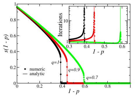
Figure 1: (Color online) Comparison between numerical and analytic results for percolation on two coupled Erdős-Rényi networks. In the main plot, the numerical (data points) results for the size of the largest connected cluster are obtained from two coupled networks with $N=512000$ nodes each and coupling strengths of $q=1,0.9,$ and $0.7$ (from left to right). The lines correspond to the analytic results computed as in Ref. Parshani2011 . The numerical results are averages over $50$ different pairs of networks and $100$ sequences of random failures. All numerical and corresponding analytic curves overlap. In the inset we see the number of iterations per failure, defined as the number of times a cascade triggered by a node failure propagates back and forth between the two networks. The lines tag the analytic results for the percolation threshold. Initially, a node removal does not trigger any cascade but, as one approaches the percolation threshold, very large cascades occur, resulting in the collapse of the entire system.

Figure 1 shows the dependence of the fraction of nodes in the largest connected cluster $s$ on the fraction of removed nodes $1-p$, for two Erdős-Rényi networks with more than one million nodes. When nodes are randomly removed, the largest connected component decreases in size, until the network is completely fragmented above a threshold $1-p_{c}$. In the inset, we see the evolution of the number of iterations per removed node. An iteration corresponds to a set of failures in one network triggered by an internetwork coupling, i.e., by the removal of a dependency link. The number of iterations is negligibly small for low values of $1-p$ but peaks at the threshold. Following the cascade after removing a node is the most computational demanding task. Consequently, an efficient algorithm is required to identify, in a fast way, if a node removal triggers a cascade or not.

Here, we propose an efficient data structure to recognize the beginning of a cascade and identify the different fragments resulting from a node removal. Since we are interested in the evolution of the largest connected component, we only follow this cluster. Our algorithm uses a hierarchical data structure with different levels. As illustrated in Fig. 2, we choose the node with the highest degree as the root and assign to it the level $L=0$. All neighbors of this root are on the second level ($L=1$) and they are directly connected to the root. All neighbors of the second level, which have not an assigned level yet, are then placed on the third level. We proceed iteratively in the same way, until all nodes of the cluster have a level. Note that we can have links within the same level and between levels but, in the latter, the level difference is limited to unity. The depth of the level structure is the maximal distance between the root and any other node in the network. For random networks, this depth approximately scales with $\log{N}$ Albert2002 ; Newman2003 and it scales even slower for many scale-free networks Cohen2003 . Note that, in the case of $n$ coupled networks we will have $n$ different hierarchical structures, i.e., one per network, representing its largest component.

When a node in level $L$ is removed, the ordering needs to be updated. All neighbors at a higher level $L+1$ which are connected to another node in level $L$ remain in the same level, as shown in Fig. 3. The nodes in level $L+1$ which have no further neighbors in level $L$ but only in level $L+1$, need to be updated (moved one level up) as well as the entire branch connected to them. In those two cases, the size of the largest connected component in this iteration is just changed by unity (the initially removed node). If neither of those cases occurs, i.e. all neighbors have a higher level, we proceed iteratively through the branch of neighbors with a breadth first search (up in level) until we detect one node in level $L^{\prime}$ which has at least one neighbor in level $L^{\prime}$ or $L^{\prime}-1$ which is not detected by the breadth first search. In this case, the entire branch of detected nodes is updated, starting from the last node in level $L^{\prime}$. On the other hand, if no node in the branch establishes a connection with the other branches, it implies that the largest component was split into subnetworks and one has to decide which one is the largest. Then the size of the largest connected component is adjusted and all nodes reorganized (see example in Fig. 4).

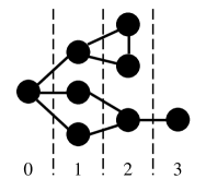
Figure 2: Example of the level structure for a small network. An energy number is assigned to each node, which corresponds to the shortest distance to the root node (the most central node in this example).

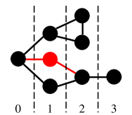
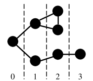
Figure 3: (Color online) Example of a node removal. In this case, the red (light) node with $L=1$ is removed. Since the only neighbor of this node with higher level has another neighbor with $L=1$, the size of the largest connected cluster is only reduced by one.

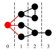
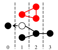
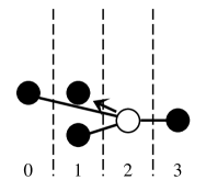
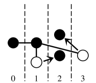
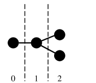
Figure 4: (Color online) Example of a reorganization due to a node removal. In the example, the root node is removed, thus the level structure has to be reorganized. First, the largest subnetwork is identified and all the other subnetworks are removed. One of the surviving first neighbors of the old root is randomly selected to become the new root. Then the levels of its neighbors are updated as well as their branches. Note that the update of a branch is complete when the level of a node remains the same. In the worst case scenario, the complexity of the entire update process is $O(M)$, where $M$ is the size of the entire branch.

III Number of commands and computational time

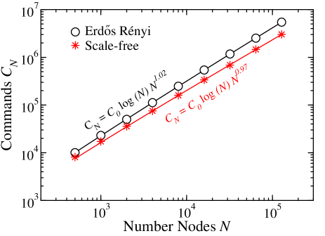
Figure 5: (Color online) The number of used commands in the program $C_{N}$ versus the system size $N$. The function $f(N)=C_{0}\log(N)N^{C_{1}}$ is fitted to the observed values. The fitting parameter $C_{1}$ is $1.02\pm 0.03$ for Erdős-Rényi networks and $0.97\pm 0.04$ for scale-free networks, respectively.

To assess the efficiency of the algorithm, we study the dependence of the number of commands $C_{N}$ on the network size $N$. We count as a command, every time a node in one of the networks is removed, its level changed, or just checked during the reorganization of the level structure. Figure 5 (main plot) shows the size dependence of the average $C_{N}$ for two coupled Erdős-Rényi networks Erdos1960 . The line fitting the data points is $C_{0}\log(N)N^{C_{1}}$, where $C_{1}$ is $1.02\pm 0.03$. In a greedy algorithm where the largest connected cluster is recalculated by counting all remaining nodes in this component after each node removal, the number of commands is expected to scale as $O(N^{2})$. With our data structure, this limit where all nodes are checked, would correspond to the worst case scenario, where the removed nodes would systematically be the root. Therefore, our algorithm represents a significant improvement over the traditional greedy algorithm. Also in Fig. 5, we plot the number of commands $C_{N}$ for two coupled scale-free networks, with degree exponent $\gamma=2.5$ Molloy1995 . The same scaling with the network size was found, with $C_{1}=0.97\pm 0.04$. So, for the two considered types of networks, our algorithm scales with $O(N\log{N})$. In general, this scaling will depend on how the average shortest path scales with the network size.

Figure 6 shows the size dependency of the average computational time $t(N)$ required to compute an entire sequence of node removals. We show the ratio $t(N)/t(N/2)$ obtained from two computers with $6$ MB and $12$ MB CPU cache for Erdős-Rényi networks (main plot) and scale-free networks (inset). In both cases, we observe a crossover between two different scaling regimes at a certain system size $N^{*}$. This crossover at $N^{*}=4000$ and $N^{*}=8000$ for $6$ MB cache and $12$ MB cache, respectively, depends on the size of the CPU cache memory (L$2$). For network sizes $N<N^{*}$, the size of the system is such that all information can be kept inside the CPU cache, being more efficient. For $N>N^{*}$, not all information fits in the CPU cache and the efficiency decreases, since the access to the Random Access Memory (RAM) is slower.

In the first regime $N<N^{*}$ the increase of the CPU time is consistent with an algorithm scaling as $O(N\log N)$. In the second regime $N\gg N^{*}$ the CPU time seems to converge to the same logarithmic scaling.

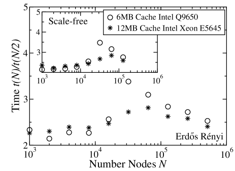
Figure 6: System-size dependence of the average CPU time $t(N)$, in seconds, necessary to calculate one sequence of node removals. We see the ratio between two times $t(N)/t(N/2)$ for two different machines (different capacity of the CPU cache memory) for two coupled Erdős-Rényi (ER, main plot) and scale-free networks (SF, inset). Results are averages over $100$ sequences of random removals and $50$ different networks.

IV Final remarks

We have proposed an efficient algorithm to monitor the size of the largest connected component during a sequence of node failures, in a system of interdependent networks. Although, in general, the algorithm can be considered to study percolation in both isolated and coupled networks, its is tailored for coupled ones. We have shown that the algorithm complexity is $O(N\log N)$, a significant improvement over the greedy algorithm of complexity $O(N^{2})$.

With our efficient algorithm, it is now possible to simulate much larger system sizes, a relevant feature to develop accurate studies. One of the most striking results of coupled networks is that, for strong coupling, the fragmentation of the network into pieces occurs in a discontinuous way Buldyrev2010 . The possibility of accurate measurements, with reduced finite-size effects, permits to determine with high precision the critical coupling above which the percolation transition is discontinuous Parshani2010a . Our algorithm can now be applied to any network topology, sequence of failures (e.g., random or high-degree node) Schneiderpre , and distribution of dependency links Li2012 , helping clarifying how to mitigate the systemic risk stemming from interdependencies.

V Acknowledgment

We acknowledge financial support from the ETH Risk Center, from the Swiss National Science Foundation under contract 200021 126853 and by New England UTC Year 23 grant, awards from NEC Corporation Fund, the Solomon Buchsbaum Research Fund.

References

- (1) A.-L. Barabási and R. Albert, Science 286, 509 512 (1999).
- (2) D. J. Watts, Small Worlds: The Dynamics of Networks Between Order and Randomness, Princeton Univ Press, Princeton (1999).
- (3) S. N. Dorogovtsev and J. F. F. Mendes, Evolution of Networks: From Biological Nets to the Internet and WWW, Oxford University Press, New York (2003).
- (4) G. Caldarelli, Scale-Free Networks: Complex Webs in Nature and Technology, Oxford University Press, New York (2007).
- (5) A. Barrat, M. Barthelemy and A. Vespignani, Dynamical Processes on Complex Networks, Cambridge Univ. Press (2008).
- (6) S. V. Buldyrev, R. Parshani, G. Paul, H. E. Stanley, and S. Havlin, Nature 464, 1025-1028 (2010).
- (7) S. W. Son, G. Bizhani, C. Christensen, P. Grassberger, and M. Paczuski, EPL 97, 16006 (2012).
- (8) C. M. Schneider, N. A. M. Araújo, S. Havlin and H. J. Herrmann, arXiv:1106.3234.
- (9) C. M. Schneider, A. A. Moreira, J. S. Andrade Jr., S. Havlin and H. J. Herrmann, Proc. Nat. Acad. Sci. USA 108, 3838 (2011).
- (10) A. Vespignani, Nature 464, 984-985 (2010).
- (11) J. Gao, S. V. Buldyrev, H. E. Stanley, and S. Havlin, Nat. Phys. 8, 40 (2012).
- (12) S. Havlin, N. A. M. Araújo, S. V. Buldyrev, C. S. Dias, R. Parshani, G. Paul, and H. E. Stanley, Catastrophic Cascade of Failures in Interdependent Networks, Complex Materials in Physics and Biology. Proceedings of the International School of Physics “Enrico Fermi”, course CLXXVI, 176, 311 (2012).
- (13) R. Parshani, S. V. Buldyrev, S. Havlin, Phys. Rev. Lett. 105, 048701 (2010).
- (14) S. W. Son, P. Grassberger, and M. Paczuski, Phys. Rev. Lett. 107, 195702 (2011).
- (15) M. Barthelemy, Phys. Rep. 499, 1 (2011).
- (16) J. Gao, S. V. Buldyrev, S. Havlin, and H. E. Stanley, Phys. Rev. Lett. 107, 195701 (2011).
- (17) X. L. Xu et al., EPL 93, 68002 (2011).
- (18) C. D. Brummitt, R. M. D’Souza, and E. A. Leicht, Proc. Nat. Acad. Sci. USA 109, E680 (2012).
- (19) P. Holme, B. J. Kim, C. N. Yoon and S. K. Han, Phys. Rev. E 65, 056109 (2002).
- (20) C. M. Schneider, T. Mihaljev, S. Havlin and H. J. Herrmann, Phys. Rev. E 84, 061911 (2011).
- (21) C. M. Schneider, T. Mihaljev and H.J . Herrmann, Europhys. Lett. 98, 46002 (2012).
- (22) R. Parshani, S. V. Buldyrev and S. Havlin, Proc. Natl. Acad. Sci. USA 108, 1007 (2011).
- (23) R. Albert and A.-L. Barabási, Rev. Mod. Phys. 74, 47 (2002).
- (24) M. E. J. Newman, SIAMReview 45, 167 (2003).
- (25) R. Cohen and S. Havlin, Phys. Rev. Lett. 90, 058701 (2003).
- (26) P. Erdős and A. Rényi, Publ. Math. Inst. Hung. Acad. Sci. 5, 17 (1960).
- (27) M. Molloy and B. Reed, Random Struct. Algorithms 6, 161 (1995).
- (28) W. Li, A. Bashan, S. V. Buldyrev, H. E. Stanley, and S. Havlin, Phys. Rev. Lett. 108, 228702 (2012).