The intriguing stellar populations in the globular clusters NGC 6388 and NGC 6441^∗

Abstract

NGC 6388 and NGC 6441 are two massive Galactic bulge globular clusters which share many properties, including the presence of an extended horizontal branch (HB), quite unexpected because of their high metal content. In this paper we use HST’s WFPC2, ACS, and WFC3 images and present a broad multicolor study of their stellar content, covering all main evolutionary branches. The color-magnitude diagrams (CMDs) give compelling evidence that both clusters host at least two stellar populations, which manifest themselves in different ways. NGC 6388 has a broadened main sequence (MS), a split sub-giant branch (SGB), and a split red giant branch (RGB) that becomes evident above the HB in our data set; its red HB is also split into two branches. NGC 6441 has a split MS, but only an indication of two SGB populations, while the RGB clearly splits in two from the SGB level upward, and no red HB structure. The multicolor analysis of the CMDs confirms that the He difference between the two main stellar populations in the two clusters must be similar. This is observationally supported by the HB morphology, but also confirmed by the color distribution of the stars in the MS optical band CMDs. However, a MS split becomes evident in NGC 6441 using UV colors, but not in NGC 6388, indicating that the chemical patterns of the different populations are different in the two clusters, with C, N, O abundance differences likely playing a major role. We also analyze the radial distribution of the two populations.

Table 1
Log of HST Observations for NGC 6388
GO	PI	Instrument	Filter	Exposures	$\Delta$r†	Epoch
(1)	(2)	(3)	(4)	(5)	(6)	(7)
9835	G. Drukier	ACS/HRC	F555W	51$\times$155 s	$0\farcm 05$	30 Oct 2003
			F814W	5$\times$25 s, 2$\times$469 s, 10$\times$505 s	$0\farcm 05$	30 Oct 2003
10350	H. Cohn	ACS/HRC	F330W	2$\times$1266 s 4$\times$1314 s	$0\farcm 05$	7 Apr 2006
			F555W	3$\times$155 s	$0\farcm 05$	7 Apr 2006
		ACS/WFC	F660N	2$\times$1123 s, 4$\times$1171 s	$4\farcm 05$	7 Apr 2006
10474	G. Drukier	ACS/HRC	F814W	5$\times$25 s, 8$\times$501 s, 4$\times$508 s	$0\farcm 05$	4–8 Apr 2006
9821a	B. Protz	ACS/WFC	F435W	6$\times$11 s	$0\farcm 08$	2003–2004
			F555W	6$\times$7 s	$0\farcm 08$	2003–2004
10775	A. Sarajedini	ACS/WFC	F606W	1$\times$40 s, 5$\times$340 s	$0\farcm 27$	6 Apr 2006
			F814W	1$\times$40 s, 5$\times$350 s	$0\farcm 27$	7 Apr 2006
11739	G. Piotto	ACS/WFC	F475W	4$\times$788 s	$3\farcm 86$	3 Jul 2010
			F814W	1$\times$67 s, 4$\times$155 s	$4\farcm 02$	30 Jun 2010
		WFC3/UVIS	F390W	6$\times$880 s	$2\farcm 35$	3 Jul 2010
		WFC3/IR	F160W	6$\times$199 s, 4$\times$249 s	$2\farcm 18$	30 Jun 2010
$\dagger$ Average distance of data set from cluster center.
aSNAP program.

Table 2
Log of HST Observations for NGC 6441
GO	PI	Instrument	Filter	Exposures	$\Delta$r†	Epoch
(1)	(2)	(3)	(4)	(5)	(6)	(7)
5667	B. H. Margon	WFPC2	F336W	2$\times$500 s	$0\farcm 05$	8 Aug 1994
8251	H. A. Smith	WFPC2	F439W	3$\times$50 s, 15$\times$80 s	$0\farcm 10$	1999–2000
			F555W	18$\times$10 s	$0\farcm 01$	1999–2000
8718	G. Piotto	WFPC2	F336W	1$\times$260 s, 2$\times$400 s	$0\farcm 02$	16 Sep 2001
9835	G. Drukier	ACS/HRC	F555W	36$\times$240 s	$0\farcm 07$	1 Sep 2003
			F814W	5$\times$40 s, 1$\times$413 s, 10$\times$440 s	$0\farcm 07$	1 Sep 2003
10775	A. Sarajedini	ACS/WFC	F606W	1$\times$45 s, 5$\times$340 s	$0\farcm 27$	25 May 2006
			F814W	1$\times$45 s, 5$\times$350 s	$0\farcm 27$	25 May 2006
11739	G. Piotto	ACS/WFC	F475W	3$\times$768 s, 3$\times$803 s	$3\farcm 86$	4–8 May 2010
				1$\times$765 s, 1$\times$800 s	$3\farcm 86$	30 May 2011
			F814W	2$\times$67 s, 6$\times$155 s	$4\farcm 02$	4–8 May 2010
				2$\times$155 s	$4\farcm 02$	30 May 2011
		WFC3/UVIS	F390W	9$\times$884 s	$2\farcm 35$	4–8 May 2010
				3$\times$884 s	$2\farcm 35$	30 May 2011
		WFC3/IR	F160W	8$\times$199 s, 8$\times$249 s	$2\farcm 18$	7 May 2010
$\dagger$ Average distance of data set from cluster center.

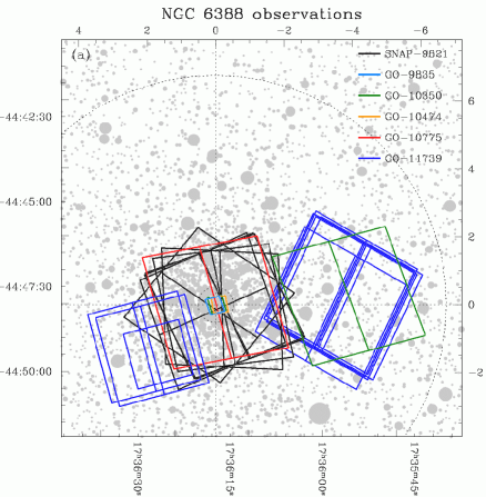
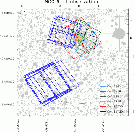
Figure 1: Finding charts for NGC 6388 (a) and NGC 6441 (b) superimposed on star maps from the $J$-band 2MASS catalog. Data sets are color-coded according to the GO program. There is no ambiguity in using the same color for different cameras (e.g., for GO-11739 WFC3/UVIS, WFC3/IR, and ACS/WFC) because of the different size of each camera’s FoV (which are shown, to scale, on the right edge of the figure). ACS/WFC is the larger 2-CCD footprint, and WFC3/UVIS is the smaller one; the larger 1-CCD footprint is WFC3/IR, and the smaller one is ACS/HRC (always placed at the cluster center). Finally, WFPC2 has its own distinctive L-shaped footprint, and is used here only for NGC 6441. We give both right ascension and declination (lower abscissa and left ordinate) and components relative to the cluster center in arcmin (upper abscissa and right ordinate). The inner dotted circle marks the half-light radius $r_{\rm h}$, while the outer one marks the tidal radius ($r_{\rm t}$, from Harris 1996, 2010 edition). The core radius (not marked) falls within the ACS/HRC pointings.

1 Introduction

Since the 1990s, NGC 6388 ($l=345^{\circ}\!\!.56$, $b=-6^{\circ}\!\!.74$) and NGC 6441 ($l=353^{\circ}\!\!.53$, $b=-5^{\circ}\!\!.01$) have been considered as “twin” clusters because of many common features. They are both located in the bulge of our Galaxy, they are two of the most luminous and massive ($\sim$1.6$\times$10⁶ M_⊙, Pryor & Meylan 1993) globular clusters (GCs) of the Milky Way, and they are both metal rich ([Fe/H]=$-$0.55 for NGC 6388 and [Fe/H]=$-$0.46 for NGC 6441, Harris 1996, 2010 edition). Despite their high metal content, their most intriguing common property is an extended blue horizontal branch (HB, Rich et al. 1997), which makes them among the most extreme examples of the so-called second-parameter problem. Moreover, the red clump (RC) of the HB is noticeably tilted, with bluer stars being brighter (in the optical bands) than redder ones (Raimondo et al. 2002).

Since the work of Rich et al. (1997), attempts to understand what is special about these two clusters have focused on these two peculiarities. Sweigart & Catelan (1998) first proposed high helium as the origin of the blue HB extension, in a scenario in which the envelope of fast-rotating stars, while ascending the red giant branch (RGB), would be enriched in helium by meridional currents. Others, focusing on the HB tilt, argued for differential reddening (DR) as the cause of the tilt itself (e.g., Raimondo et al. 2002), but even though these clusters are certainly affected by DR, the size of the tilt is too large to be explained by DR alone, and finally, DR has been excluded by Busso et al. (2007), who found that the HB tilt persisted in all parts of their field, in each of the two clusters.

It became evident that traditional evolutionary scenarios could not account for the properties of these two clusters following the discovery that their RR Lyrae variables have exceptionally long periods (something that could be explained by high helium but certainly not by DR). With an average fundamental-mode period of $\langle P_{ab}\rangle=0\fd 71$ for NGC 6388, and $0\fd 76$ for NGC 6441, these two clusters were legitimately considered to be the prototype of a third Oosterhoff type (the average periods of Oosterhoff I and Oosterhoff II clusters being $0\fd 55$ and $0\fd 65$, respectively, Layden et al. 1999; Pritzl et al. 2000, 2001, 2002, 2003).

The discovery of multiple stellar populations with enhanced helium in several GCs (see Piotto 2009 for a recent review) offers a new perspective for understanding the many apparent anomalies that these two clusters share. After it was shown that high helium could be the cause of both the blue HB extension and the unusual period of the RR Lyrae (D’Antona & Caloi 2004; Caloi & D’Antona 2007; Busso et al. 2007), the question became whether high helium was the result of deep-mixing in a minority of RGB stars (as originally suggested by Sweigart & Catelan 1998), or was due to the presence of a second, helium-enriched stellar population. In the former case no splitting of the main sequence (MS) was expected, whereas a sizable split should exist if the blue HB and RR Lyrae stars belong to a distinct, helium-rich sub-population.

Evidence for different stellar generations has already been found in both clusters with the detection of light-element star-to-star variations and the Na–O anticorrelation (Gratton et al. 2007; Carretta et al. 2007, 2009a). Moreover, NGC 6388 also exhibits a split sub-giant branch (SGB, Piotto 2008; Moretti et al. 2009; Piotto et al. 2012). Thus, if the blue HB and RR Lyrae stars belong to helium-enriched populations in these clusters, we should be able to see the effect of enhanced He on the MSs (a spread or a split), to quantify the enhancement, and to check whether it is consistent with the amount of helium enhancement required to account for the HB properties.

To this end, we submitted a Hubble Space Telescope (HST) proposal (GO-11739, PI G. Piotto) to perform accurate photometry of NGC 6388 and NGC 6441 with the Wide Field Camera 3 (WFC3). In the present paper, we combine GO-11739 data with a large set of archival images from the Advanced Camera for Surveys (ACS) and the Wide-Field Planetary Camera 2 (WFPC2), in order to thoroughly map the multiple stellar populations of these two clusters from their MS all the way to the SGB, RGB and HB.

This paper is organized as follows: in Section 2 the vast set of HST data used for the project is presented, along with the reduction procedures. In Section 3 distinct stellar populations are identified in all the color-magnitude-diagram (CMD) sequences of the two clusters, and in Section 4 their radial distributions within the clusters are presented. In Section 5 we estimate the the amount of helium enhancement $\Delta Y$ required to account for the size of the MS split, and discuss its implications at the light of our new observational findings.

2 Data sets and reductions

This work is based on proprietary and on archival HST images. We made use of exposures taken with three different cameras: (1) ACS, with both the Wide-Field Channel and the High-Resolution Channel (WFC and HRC); (2) WFC3, with both the Ultraviolet-Visible (UVIS) and the Infrared (IR) channels; and (3) WFPC2. A list of the observations is given in Table 1 for NGC 6388 and in Table 2 for NGC 6441.

To summarize briefly: ACS/WFC observations come from programs SNAP-9821, GO-10775 and GO-11739 for NGC 6388; from GO-10775 and GO-11739 for NGC 6441. ACS/HRC observations are from programs GO-9835, GO-10350, and GO-10474. WFPC2 exposures come from GO-5667, GO-8251, and GO-8718. Much of our material is archival, but as an essential part of this study we specifically designed the new program GO-11739 (PI: Piotto) to detect multiple stellar populations along the MSs of NGC 6388 and NGC 6441 by exploiting the power of the new WFC3 cameras. We used both WFC3/UVIS and WFC3/IR, in each case taking parallel exposures with ACS/WFC.

Figure 1 shows the footprints of all exposures that are listed in Tables 1 and 2, superimposed on stars from the 2MASS $J$-band catalog. A distinctive color is used for each program and a distinctive shape and size for each camera.

Figure 1 and Tables 1 and 2 are crucial for this paper, as they exhibit the overlaps of the different data sets, which govern much of what follows. Careful study of the figure, along with the tables, will enable the reader to see possible filter combinations that can be used to build CMDs at different radial locations in the clusters. Moreover, since some overlapping data sets encompass different epochs, one can see where proper motions are measurable, information that will prove invaluable for selection of cluster members. The reader should particularly note, for each cluster, the overlap between GO-11739 and GO-10775 (much smaller for NGC 6388 than for NGC 6441).

In this paper we will focus our attention on the more central fields, leaving the analysis of the outer fields to a later paper. This choice will not affect our results, since the outer field has been imaged only with filters not designed to highlight the multi-population phenomenon along the MS of these two clusters. Moreover, the outer field does not have enough RGB and SGB stars for a study of their radial distribution.

2.1 ACS/WFC and HRC

All ACS/WFC _flt images (i.e., images that were dark- and bias-subtracted and flat-fielded, but not resampled) were corrected for charge-transfer deficiencies by using the procedure and the software developed by Anderson & Bedin (2010).

Photometry and astrometry were carried out with the software tools described by Anderson et al. (2008). Briefly, all exposures belonging to a specific program were analyzed simultaneously to generate an astrophotometric catalog of stars in the field of view (FoV). Stars were measured independently in each image by using the spatially varied point-spread function (PSF) library models from Anderson & King (2006b), along with a spatially constant perturbation specifically derived for each exposure, to compensate for small focus changes due to spacecraft “breathing”. Star positions were corrected for geometric distortion using Anderson & King (2006b) and Anderson (2007).

Photometry was calibrated into the Vega-mag flight system following recipes in Bedin et al. (2005), and using the zero points given in Sirianni et al. (2005).

The measurement of stellar fluxes and positions in each ACS/HRC image was performed by using the publicly available routine img2xym_HRC, library PSFs, and the distortion correction described in Anderson & King (2006a). We corrected the photometric zero points in the same way as for the WFC photometry.

2.2 WFPC2

The WFPC2 images are not _flt-type (introduced only for later instruments), but rather the earlier equivalent _c0f. We reduced them with the algorithms described in Anderson & King (2000). The field was calibrated to the photometric Vega-mag flight system of WFPC2 according to the prescriptions of Holtzman et al. (1995).

2.3 WFC3/UVIS and IR

For the WFC3 exposures we used the _flt images. Star positions and fluxes on WFC3/UVIS images were measured with software based mostly on img2xym_WFI (Anderson et al. 2006), which implements a set of spatially variable empirical PSFs for each individual exposure. We corrected positions for geometric distortion using the recipes given in Bellini & Bedin (2009) and Bellini, Anderson & Bedin (2011). Photometry was calibrated as in Bedin et al. (2005).

Infrared images were reduced with software based on that of Anderson & King (2006a) for ACS/HRC. We constructed an empirical F160W “effective PSF” using the 3-step procedures devised by Anderson & King (2000). A detailed description of the software, PSF derivation, and geometric distortion solution will be presented elsewhere. Photometry was calibrated as in Bedin et al. (2005).

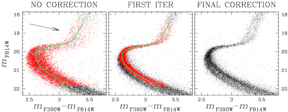
Figure 2: Illustrating the correction for differential reddening. The first panel shows the uncorrected $m_{\rm F814W}$ vs. $m_{\rm F390W}-m_{\rm F814W}$ CMD of NGC 6441 around the SGB region. Stars used as a reference for the first-guess DR correction are marked in red, and the fiducial sequence in green. The arrow shows the direction of the reddening vector. After a trial correction (second panel), the sequences in the CMD are significantly narrower, and we are able to refine our choice of reference stars and adjust the fiducial sequence a little. In the final panel is the result of three iterations. Note the sharpness of the SGB, and the splits in the MS and RGB.

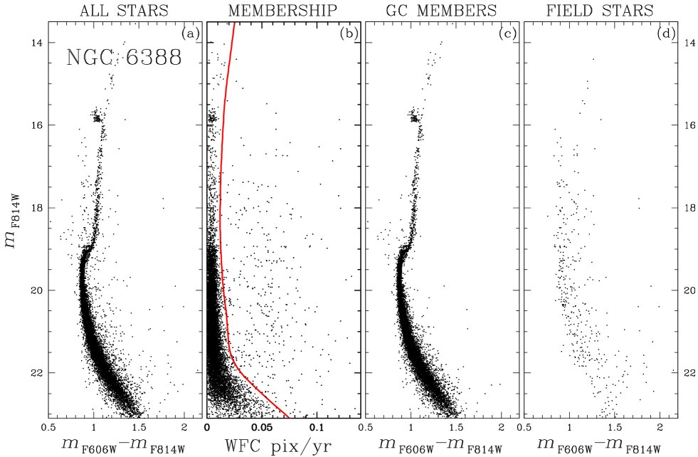
Figure 3: Illustrating the proper-motion separation for NGC 6388. (a) CMD for stars in common between GO-10775 and GO-11739. (b) Sizes of the proper-motion displacements (in pixel/yr); the red line (drawn by hand) shows our membership criterion. (c) CMD of proper-motion-selected cluster members; (d) stars rejected as field stars (even though this means the loss of a few members).

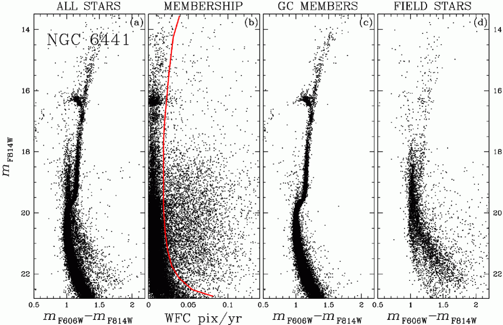
Figure 4: Same as Fig. 3, but for NGC 6441. Although the field contamination is much stronger, we have nevertheless selected an almost clean sample of cluster members.

2.4 Sample selections

Since our aim is fine photometric discrimination, it was a great advantage to select the best-measured stars in our samples. To accomplish this, we closely followed the recipes and used the same selection criteria as given in Milone et al. (2009), which makes use of several diagnostics: photometric and astrometric rms, PSF-fit residuals, and amount of scattered light from neighboring stars. (This last diagnostic is available only for ACS/WFC catalogs because, as we stated above, different codes where used for different cameras, and only the one for the ACS/WFC provides the additional diagnostic.)

For more information about our selection procedures we refer the reader to Milone et al. (2009).

2.5 Differential reddening

Both NGC 6388 and NGC 6441 are in the direction of the Galactic bulge, where extinction is a serious problem ($E(B-V)$ 0.37 and 0.47 respectively, according to Harris 1996, 2010 edition). Such large reddenings can be expected to be accompanied by serious differential reddening, which we treated with particular care.

As a first step, for each CMD we computed the direction of the reddening vector. For this we used the extinction coefficients in Tables 14 and 15 of Sirianni et al. (2005) for G2 stars. For WFC3 F390W, which is not in those tables, we interpolated linearly between ACS/HRC F330W and F435W, getting $A_{\rm F390W}/E(B-V)=4.49$. For the F160W filter we adopted the value $A_{\rm F160W}/E(B-V)=0.57$ (from YES, the York Extinction Solver), and used the Fitzpatrick (1999) extinction law. As we did for the WFPC2, we took the extinction values from Schlegel, Finkbeiner & Davis (1998).

We dealt with differential reddening (DR) by means of a method that is explained in detail in Section 3.1 of Milone et al. (2012a), to which we refer the reader for details; here we only describe the method briefly.

The overall method consists of iterating a core procedure which itself has five steps: (1) We rigidly rotate the CMD to make the reddening direction parallel to the $x$ axis, so that DR becomes a simple shift in $x$, and the $x$ distance of a star from the now-vertical fiducial becomes an estimate of its DR value. (2) We next choose a set of “reference stars” — stars whose DR values are best suited to serve as standards. Ideally these stars should lie in the parts of the CMD where the sequences are almost perpendicular to the reddening vector, i.e., the SGB and the faint parts of the RGB; to get enough reference stars, however, we had to include the upper part of the MS. (3) We draw a fiducial line along the MS, SGB, and RGB using reference stars. (4) Our actual DR correction makes use of the fact that DR varies systematically with position in the field. What we do is to correct the color of each star by the median reddening of the nearest $n_{\ast}$ reference stars (see below). (5) We rotate the corrected values (i.e., corrected $x$ and unchanged $y$) back into the CMD frame.

A final step in each iteration was to redraw the fiducial sequence in reaction to the changes in the choice of reference stars. (In practice, changes after the first iteration are trivial, though.)

For any CMD that we need to correct, we choose $n_{\ast}$ by trial and error, as a compromise between a large $n_{\ast}$ for robustness and a small one for spatial resolution. Typical $n_{\ast}$ values are in the range 50–70.

The reason we need to iterate the process is to optimize the choice of the set of reference stars. As this choice improves, the DR correction gets better, and the sequences in the corrected CMD get sharper, allowing a more perceptive choice of reference stars — and so on, until the choice of reference stars no longer improves. It is important to keep in mind, however, that the DR correction is always made to the original photometry, but with the new reference stars; it is the optimization of the reference stars that makes the method work.

We illustrate this procedure with our DR correction of NGC 6441, several steps of which are shown in Figure 2. The first panel shows the $m_{\rm F814W}$ vs. $m_{\rm F390W}-m_{\rm F814W}$ CMD of the cluster around the SGB region, with our initial choice of reference stars marked in red, and our initially-drawn fiducial sequence in green.

The next panel shows the result of the first application of the procedure; the DR correction was good enough to produce a significant narrowing of all the sequences in the CMD; moreover, the RGB is now bimodal, and the MS is showing suggestions of bimodality. This improvement allows us to choose a new set of reference stars (marked in red), from which we have removed stars of the blue MS, and a number of binaries and field stars. The green line is the redrawn fiducial sequence.

As indicated, we iterated this procedure. Three iterations were enough to reach our final choice of reference stars and the consequent DR correction. (A fourth iteration yielded negligible improvement.) The final DR-corrected CMD is shown in the right panel of Fig. 2.

Our procedure also allows us to construct reddening maps, by averaging the DR value used to correct the stars in each region. (Note that we will return to this subject in Sect. 3.3, to present a specific validation of the NGC 6441 reddening map.)

Finally, we note that from this point on, all the CMDs that we show are corrected for differential reddening.

2.6 Proper motions

As noted in an earlier subsection, field-star contamination presents a serious problem in our analysis of the fine structure of the CMDs. There is no problem for the ACS/HRC and WFPC2 fields, which are at the cluster centers, where field stars represent a negligible fraction. The issue arises when we analyze ACS/WFC data (in particular GO-10775) and the new WFC3 exposures (GO-11739), which were taken off-center to avoid crowding. Since the GO-10775 and GO-11739 exposures overlap for both clusters, we were able to measure proper motions, with a baseline of at least 4 years. In addition, some of GO-11739 exposures of NGC 6441 were purposely taken a year apart, in order to measure proper motions in the parallel ACS/WFC field, where it was clear that field-star contamination was very serious. This provides us with up to 5 years of time baseline between GO-10775 and GO-11739 for NGC 6441 (and of course the 1-year baseline within GO-11739 — needed for CMDs that use only that program).

Proper motions were measured using ACS/WFC F606W and F814W exposures as first epoch and WFC3/UVIS F390W exposures as second epoch. We did not use WFC3 IR exposures for proper motions, because of the more than twice-as-large pixel size of the IR detector and its severe undersampling.

We used the catalogs created by Anderson et al. (2008) to define a master coordinate frame. As we did in (e.g.) Bellini et al. (2009a), we first defined for each cluster a reference set of probable members, on the basis of their position in the $m_{\rm F814W}$ vs. $m_{\rm F606W}-m_{F814W}$ CMD. These included only bright, unsaturated stars, which have smaller position errors.

For each star we took each and every pairing of a position measurement from the first epoch and another from the second epoch, and transformed each of the two catalog positions into the master frame, by means of a six-parameter linear transformation using only a local set of 50 reference stars; we then differenced the two epochs to derive a displacement for that pairing. We took a 3$\sigma$-clipped median of all these displacements of the star, and assigned it a sigma that was the 68.27 percentile of the residuals around the median. Since the reference stars are nearly all cluster members, the displacements of stars are all relative to the mean motion of the cluster.

After this first estimate of the proper motions, we excluded from our selection of reference stars those whose motion differed from the mean by more than 3 sigmas, and re-derived the motions. After three iterations the process converged.

Even though the mean motions of both NGC 6388 and NGC 6441 are similar to the motions of the field stars, the dispersion of internal motion in each cluster is about five times smaller than that of field stars ($\sim$18 km/s vs. 100 km/s). Thus by selecting stars whose motion is close to the mean motion of the cluster, we exclude the majority of field stars.

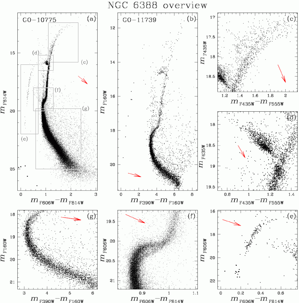
Figure 5: Overview of the main features in the CMDs of NGC 6388, from different combinations of magnitude and color. Panel (a) shows a CMD from GO-10775 (the most complete CMD), while in (b) is the CMD from GO-11739 WFC3 (the CMD with the widest color-baseline). In (a) we have highlighted five regions, labeled (c)–(g), around main cluster features. These regions are then shown in panels (c) to (g) using the filter pairs that best enhance each CMD region, e.g., a double RGB in panel (c), or a double SGB in panel (f).

For NGC 6388, the overlap region can be seen in the left panel of Figure 1, involving the bifurcated red and the bifurcated blue footprints at the lower left. In Figure 3 we illustrate our proper-motion selection. Successive panels show the CMD of all the stars, the separation of cluster and field based on the sizes of motions, the CMD of the cluster stars, and the CMD of the field stars. From the last panel it is clear that in CMDs where we do not have proper-motion separation, the risk of field-star contamination will be greatest for the SGB and MS regions. (Note: although we had three filters available, we have chosen here to display the CMD using the more familiar F606W–F814W pairing; F390W will come into play in our ensuing discussion of the details of the sequences of the CMDs.)

Figure 4 is the analog of Fig. 3, for NGC 6441, in the overlap region of the same two programs (the same colors and shapes of footprint, near the top of the right-hand panel of Fig. 1). In this case there are many more stars, both because of a larger overlap and also because these exposures are near the cluster center. Also, field-star contamination is much more severe than for NGC 6388, making cluster-field separation for NGC 6441 even more important. Nevertheless, our proper-motion separation yields an almost clean sample of cluster members in panel (c), even though panel (d) shows that we have lost a few cluster members.

Proper-motion-selected CMDs will be used extensively throughout the paper. Note also that when proper-motion measurements were available we used them to select bona-fide cluster members as reference stars for improved DR corrections.

3 Evidence of multiple populations

In this section we marshal the resources of our cameras and filters to examine each of the clusters in detail, in order to uncover all the evidence of multiple populations that we can find. We begin with an overview of a carefully chosen array of CMDs of each cluster; then we take up the regions of the CMD in detail, one by one.

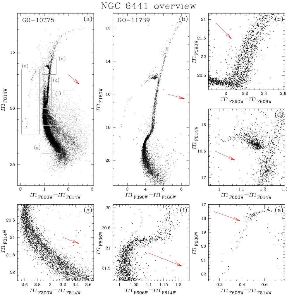
Figure 6: Overview of the main features in the CMDs of NGC 6441, as in the previous figure for NGC 6388, except that the examples of enhancement are now the double RGB in panel (c) and the double MS in panel (g).

3.1 Detailed color-magnitude diagrams of NGC 6388

Figure 5 begins with two overall CMDs of NGC 6388. In panel (a) we show the most familiar form of CMD, using F606W and F814W from the ACS/WFC images of GO-10775; it extends from the tip of the RGB down to five magnitudes below the MS turn-off. (These include the stars that we showed in the nearly identical CMD of panel 4(a), but now we include the fainter stars that did not figure in the proper-motion discussion.) Panel (b) shows a CMD from F390W and F160W of the WFC3/UVIS and IR respectively, from GO-11739; there are fewer stars here, because the smaller WFC3 images are off-center, but this is our widest color baseline, and this CMD is new.

In panels (c)–(g) we show in detail the five regions that are outlined in panel (a); for each detail panel, however, we use the combination of filters that best enhances the features of that part of the CMD. We will return to these in later subsections, but even now we readily see the splits of the RGB in (c) and the SGB in (f) as well as the complex structure of the red clump of the HB in (d). (It is not obvious, but we shall see that panel (g) shows a greater MS width than photometric errors can account for. In any case, the corresponding panel for NGC 6441 will show a clear split.) Panel (e) shows the extended blue HB, which has the anomalous blue tail of stars (highlighted by larger dots). In each panel the reddening vector is shown as a red arrow.

In these panels we have plotted only those stars less affected by the severe crowding in these central fields. We omitted stars closer to the center than a magnitude-dependent limiting radius, which we chose by hand in a way that excludes larger regions for the fainter stars.

Proper-motion selection is not used in any of the panels of this figure. The purpose of panels (a) and (b) is simply to show the whole CMD and to define panels (c)–(g). Panels (c), (d), and (e) show CMD regions where field-star contamination is minimal, while in (f) and (g) any gain in sharpness would be greatly outweighed by the loss in star numbers from cutting back to the small overlap region between the GO-10775 and GO-11739 images.

3.2 Detailed color-magnitude diagrams of NGC 6441

Figure 6 is an overview of the CMDs of NGC 6441, similar to Fig. 5 for NGC 6388.

The CMD from GO-10775 data alone (panel (a)) shows strong contamination from stars of the Galactic bulge, as already mentioned. The 1-year time span of the GO-11739 data set allowed us to remove most of the field stars from the largest-color-baseline CMD shown in panel (b). (This is why there is less field contamination here than in Fig. 5b.) Panels (a) and (b) here have the same scale as those of Fig. 5, so as to allow a direct visual comparison of the complete CMDs of these two clusters. (Similarly, in the following subsections we will show a direct comparison of the different evolutionary sequences of these clusters using CMDs with the same filters and axis scale.)

Again, in the $m_{\rm F814W}$ vs. $m_{\rm F606W}-m_{\rm F814W}$ plane we highlight five regions, labeled (c) to (g), where the main cluster CMD features are present. The CMDs zoomed around these regions are shown in the other panels of the figure, using the combinations of filters that best enhance these features, and taking advantage of proper motions to remove field stars, whenever useful (panels (c), (d), (f), and (g)).

We did not use proper-motion selections for panel (e). First, the blue HB is only marginally contaminated by field stars. Second, because proper motions are confined to the overlap area between GO-10775 and GO-11739, we would have ended up with only half as many stars, in a region of the CMD that is thinly populated. We need also to note that for panel (d), for the RC of the HB, we had to use here the $m_{\rm F814W}$ vs. $m_{\rm F606W}-m_{\rm F814W}$ CMD instead of the $m_{\rm F435W}$ vs. $m_{\rm F435W}-m_{\rm F555W}$ CMD that we used for NGC 6388, because for NGC 6441 the equivalent WFPC2 F439W images do not go deep enough.

Unlike NGC 6388, the RGB of NGC 6441 clearly splits at its base when using the F390W filter (panel (c)). Furthermore, for the first time we can see that the MS of NGC 6441 is split into two distinct sequences (panel (g), more details later).

In the following subsections we will compare and analyze each evolutionary stage of the two clusters. We want to emphasize once again that all the CMDs presented in this work are corrected for differential reddening effects.

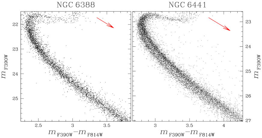
Figure 7: $m_{\rm F390W}-m_{\rm F814W}$ CMD of the upper-MS and SGB regions of NGC 6388 (left) and NGC 6441 (right), on identical scales, contrasting their sequences. As usual, reddening vectors are shown.

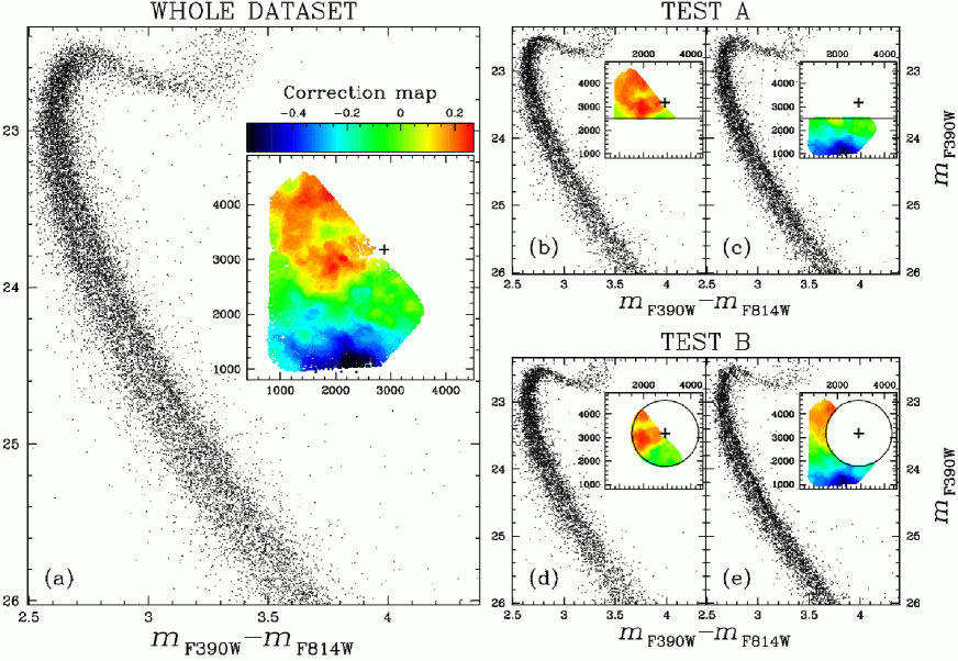
Figure 8: (a) CMD of NGC 6441 around its MS and TO; inset shows our differential reddening map, with a “+” sign at the cluster center. Panels (b)–(e) show the results of the two tests described in the text, which demonstrate that the MS width cannot be explained by differential reddening. The inset in each of those panels identifies the region whose CMD is shown.

3.3 The Main Sequences

Figure 7 shows the CMDs of NGC 6388 (on the left) and NGC 6441 (on the right) around the MS region in the $m_{\rm F390W}$ vs. $m_{\rm F390W}-m_{\rm F814W}$ plane, adopting the same axis scale. The reddening vectors are also displayed. It is clear from the figure that the MS morphology of these “twin” clusters is quite different. The MS of NGC 6388 is wider than expected from observational errors alone (more in the following), but the CMDs made using all combinations of filters at our disposal fail to provide any hints of a MS split. On the other hand, there seems to be no doubt that the MS of NGC 6441 is bimodal.

Because of the relatively high reddening values of the two clusters, one might suspect that the spread/split in the MS of the two clusters is the result of badly corrected differential reddening. We note, however, that the reddening vector runs parallel to the MS, so that reddening cannot affect the width of the MS, nor should DR correction affect it either. This near-parallelism of the reddening vector to the MS should be kept in mind, as it applies to nearly all CMDs. It will be seen, moreover, that a similar parallelism holds for the reddening vector and two-color diagrams of MS stars for all color combinations. Indeed, if we plot an uncorrected CMD of a region of NGC 6441 small enough that differential reddening cannot be an issue, the MS split is visible.

To further verify that we are not being deceived by serious systematics in our DR corrected photometry, we performed two specific tests. The left panel of Fig. 8 shows the $m_{\rm F390W}$ vs. $m_{\rm F390W}-m_{\rm F814W}$ CMD of NGC 6441 around its MS and TO regions, for all stars in common between GO-11739 and GO-10775 FoVs. (We chose these two filters because they are the only ones that clearly split the MS; we are confined to the stars in the overlap region because the two filters come from those two different programs.)

The inset shows the color-coded DR map for all the stars, in the coordinate reference system of the GO-10775 data set, with map coordinates in ACS/WFC pixels. The cluster center is marked by a “$+$”. Each point corresponds to a star, and is colored according to the DR correction found for it. The maximum extent of the DR corrections is 0.86 mag along the direction of the reddening vector.

Since the DR correction map shows a vertical gradient, for the first test (TEST A) we split the FoV into upper and lower subsets containing the same numbers of stars, and performed the DR correction procedure on each of the two independent subsets, as a test of whether the apparent breadth of the MS could be just high/low reddening. The resulting CMDs, in panels (b) and (c), each show the MS split of panel (a) — somewhat more clearly in (c), because the stars of panel (b) suffer photometrically from the crowding in the cluster center. In the less perturbed photometry of panel (c) one can even discern a dominant red component and a bluer tail in the colors. But the main point is that Test A totally refutes the idea that the bluer and redder parts of the MS spread could simply be stars with greater and less reddening.

To investigate whether the MS spread/split might in fact result directly from crowding in the cluster center, we performed TEST B, in which the two halves of the sample were an inner one and an outer one, as shown in panels (c) and (d). The MS width is still evident in both samples, and the outer sample, in panel (d), if anything shows the split even more strongly than panel (c), above it.

These tests show that the MS spread of NGC 6441 is real. Moreover, when only less-crowded, well-measured stars are selected (e.g., right panel of Fig. 7, but see also panel (a) of Fig. 8), the MS splits into two branches, the redder one being the more populated.

No MS split was visible in the case of NGC 6388, but the tests just performed can be taken as evidence that the MS broadening observed there is also real, rather than an artifact of differential reddening.

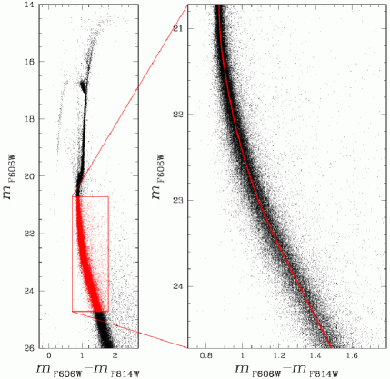
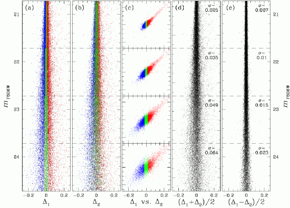
Figure 9: The two leftmost panels show the GO-10775 $m_{\rm F606W}$ vs. $m_{\rm F606W}-m_{\rm F814W}$ CMD of NGC 6388 and a zoom-in of the upper MS. The fiducial line is in red in the second panel. The remainder of the figure shows the complicated procedure that is described in the text, in which we divide the images into two sets and show that the stars show similar color residuals in the two independent data sets.

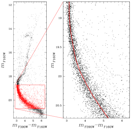
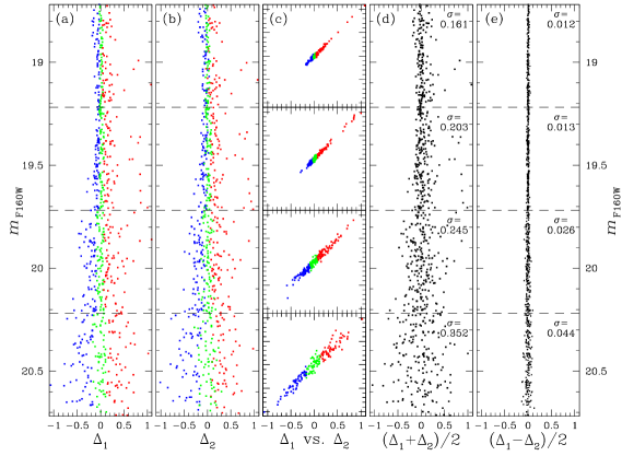
Figure 10: Same as Fig. 9, but using $m_{\rm F160W}$ vs. $m_{\rm F390W}-m_{\rm F160W}$.

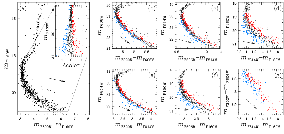
Figure 11: Multicolor analysis for the MS of NGC 6388. Panel (a): the $m_{\rm F160W}$ vs. $m_{\rm F390W}-m_{\rm F160W}$ CMD. The inset shows the rectified CMD, with blue, black, and red stars plotted in those colors. Panels (b) through (f) show CMDs using different filter combinations; the stars keep the same color coding; panel (g) is the $m_{\rm F390W}-m_{\rm F606W}$ vs. $m_{\rm F814W}-m_{\rm F160W}$ two-color diagram, showing only the blue- and red-coded stars. The two extreme groups remain distinct in all panels. Each panel includes a reddening vector.

3.3.1 The MS of NGC 6388

As shown in the study by Anderson et al. (2009) of the MS broadening in 47 Tuc, and by Milone et al. (2010b) for NGC 6752, an effective way of testing for a true CMD-sequence broadening is to divide the images of the field of stars into two independent halves. If the broadening is intrinsic, the stars that have redder (or bluer) colors in a CMD made from one half of the images will have redder (or bluer) colors in the CMD from the other half. But if the broadening is due only to measuring errors, a star that is redder in the first half of the images will have an equal chance of being redder or bluer in the second half, and the bluer stars of the first subset are equally likely to be red or blue in the second half. Again, we note that the reddening vector is almost parallel to the MS (see, e.g., panel (a) of Fig. 5), and therefore DR cannot change the locations of the stars with respect to the MS fiducial line. In the following, we will apply this technique, basically following the procedure described in Anderson et al. (2009).

The leftmost panel of Fig. 9 shows the $m_{\rm F606W}$ vs. $m_{\rm F606W}-m_{\rm F814W}$ CMD of NGC 6388. The second panel shows a zoom-in of the upper part of the MS (colored in red in the first panel). The continuous curve in red marks the adopted MS ridge line. We subtracted from the color of each star that of the MS ridge line at the same magnitude level. The rectified MS obtained in this way, for the two independent set of images, is shown in panels (a) and (b). In panel (a) the stars were divided into three equally-populated groups, color-coded in red, green and blue. In panel (b) we have kept for each star the same color that it had in panel (a). (We decided to divide the MS into three groups rather than two, as we had done in our previous papers, to better understand the color behavior of the stars in the two subset of images.)

It is clear that the color of stars is maintained very well (with only a small scatter due to photometric errors) from panel (a) to panel (b). To emphasize this fact, we show in panel (c) the correlation between the color of each star in the two halves of the data, divided in four different magnitude bins (since measuring errors increase at fainter magnitudes). A star redder than the MS ridge line in the first half of the data is also measured as redder in the great majority of cases, in the second half of the data, and vice-versa. This is the mark of a true spread in color.

In panel (d) we show the color distribution of the rectified MS as measured from the whole set of images, $(\Delta_{1}+\Delta_{2})/2$. The distribution of half the difference between the colors measured separately from each half of the images, $(\Delta_{1}-\Delta_{2})/2$, is presented in panel (e). This distribution is a statistical estimator of the error in the color distribution in panel (d).

At each magnitude level of panels (d) and (e), an estimate of the $\sigma$ of the spread of the distribution is given (calculated here as the 68.27 percentile of the absolute deviation from the median). As one can see, the intrinsic width of the MS is about three times as large as what would be expected from photometric errors alone. (As a further test, artificial stars within the magnitude interval shown in Fig. 9, and chosen to have $m_{\rm F606W}-m_{\rm F814W}$ colors along the MS of NGC 6388, gave MS widths ranging from 0.005 to 0.027 — only a small fraction of the width observed in Fig. 9.)

A similar procedure applied to the $m_{\rm F390W}-m_{\rm F814W}$ color yields a 1$\sigma$ width of the MS of 0.09 mag, at 1.1 mag below the turnoff (after subtracting in quadrature the photometric errors of $\sim 0.03$ mag).

The presence of an intrinsic breadth in the MS in NGC 6388 is further confirmed when we apply the technique of Anderson et al. (2009) to the GO-11739 data set (Fig. 10). In this case, the color baseline is six times larger, and the MS appears to be about ten times wider than what is expected from photometric errors alone.

The GO-10775 and GO-11739 fields overlap marginally (only about a thousand stars with a measure in all the 4 available filters), but this is enough to show, in Fig. 11, a multicolor analysis, similar to what was done for $\omega$ Centauri by Bellini et al. (2010), 47 Tuc by Milone et al. (2012b), and NGC 6397 by Milone et al. (2012c). Moreover, here we can use proper motions to eliminate field stars — much more important here than in the sparse fields of Milone et al.

We rectified the MS in the $m_{\rm F160W}$ vs. $m_{\rm F390W}-m_{\rm F160W}$ plane, in the magnitude interval $18.75<m_{\rm F160W}<21$ (see panel (a) and the inset of Fig. 11). Note that at $m_{\rm F160W}>20.5$ the MS is already as wide as about 1 magnitude in the proper-motion-selected CMD. We defined three groups of stars (marked with blue, black, and red colors), with the property of being bluer, of average color, and redder, respectively, than an arbitrary line drawn through the middle color of the MS (not shown in the Figure). We then kept the same colors for the stars of these two groups in plotting different CMDs (panels (b) through (f)), made by using all other available color combinations. A final panel (g) shows the two-color diagram $m_{\rm F390W}-m_{\rm F606W}$ vs. $m_{\rm F814W}-m_{\rm F160W}$ for the two extreme groups of stars. It is interesting to note that blue and red stars always remain on the blue and on the red side of the MS, respectively. The reddening vectors are drawn in order to emphasize that they are approximately, or even closely, parallel to the faint MS in the CMDs and, most importantly, in the two-color diagram. Thus differential reddening has little or no effect on the MS width or on the separation of the red and blue points.

We have demonstrated that the MS of NGC 6388 shows a significant color spread. This can be seen both by using optical colors and, more importantly, by using the wide color baseline offered by the new GO-11739 F390W and F160W images. Even so, our careful investigation was unable to reveal any hint of MS splitting with the data sets at our disposal.

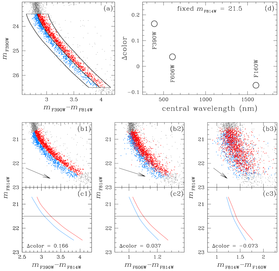
Figure 12: Multicolor analysis of the MS of NGC 6441. The two MS populations are selected in panel (a). Panels (b) and (c) show the behavior of the sequences and their fiducials in the planes $m_{\rm F814W}$ vs. $m_{\rm X}-m_{\rm F814W}$, where X is one of the other filters. The color differences between the two sequences at fixed $m_{\rm F814W}=21.5$ are plotted in panel (d).

3.3.2 The MS of NGC 6441

In NGC 6388 we were able only to demonstrate that the MS is broad, without managing to reveal possible MS subpopulations. In NGC 6441, by contrast, the MS components are visibly split, and we can therefore study their behavior in a much more straightforward way. What is more, GO-10775 and GO-11739 overlap by about half the ACS/WFC field — much more than in the case of NGC 6388 — and this makes for much better statistics. What we do for NGC 6441, then, is to perform a multicolor analysis in order to model the difference in the chemical content of the two MS populations, as we did in 47 Tuc (Milone et al. 2012b) and NGC 6397 (Milone et al. 2012c).

We drew a fiducial line by hand passing in between the two MSs, and defined as rMS stars those within a 0.2-mag interval of color redward from this fiducial, and as bMS stars those within 0.2 mag blueward from it, in the magnitude interval $23.5<m_{\rm F390W}<26.5$ (see panel (a)) of Fig. 12).

Panels (b) show the $m_{\rm F814W}$ vs. $m_{\rm X}-m_{\rm F814W}$ CMDs of the two MSs, where X is one of the other three filters (F390W, F606W, and F160W). In panels (c) we plotted the location of the ridge lines of the two MSs in the same planes as panels (b). We measured the color difference $\Delta$color between the blue and the red ridge lines at a fixed magnitude level ($m_{\rm F814W}=21.5$, black horizontal lines). Panel (d) collects these color differences as a function of the central wavelength $\lambda$ of the $m_{\rm X}$ band (open circles).

The color difference between the two sequences depends strongly on the adopted color baseline. In particular, it is highest in the $m_{\rm F390W}-m_{\rm F814W}$ color, where it amounts to $\sim 0.166$ mag (1.1 mag below the turnoff). This compares to 0.09 mag as the width of the MS of NGC 6388 and we conclude that the MSs of the two clusters are intrinsically different, with the MS of NGC 6388 being narrower than the separation of the two MSs of NGC 6441. We will demonstrate in Section 5 that:

• The color spread of the MSs of the two clusters is similar in $m_{\rm F606W}-m_{\rm F814W}$, implying that the difference in He content among the different stellar populations in the two clusters must be similar (as strongly suggested by the morphology of their HBs);

• Other chemical differences (which would be C, N, and O) must be invoked to explain the sharp difference of the two MSs in the $m_{\rm F814W}$ vs. $m_{\rm F390W}-m_{\rm F814W}$ CMD.

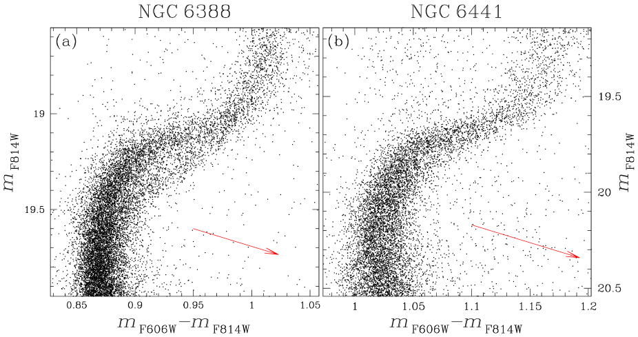
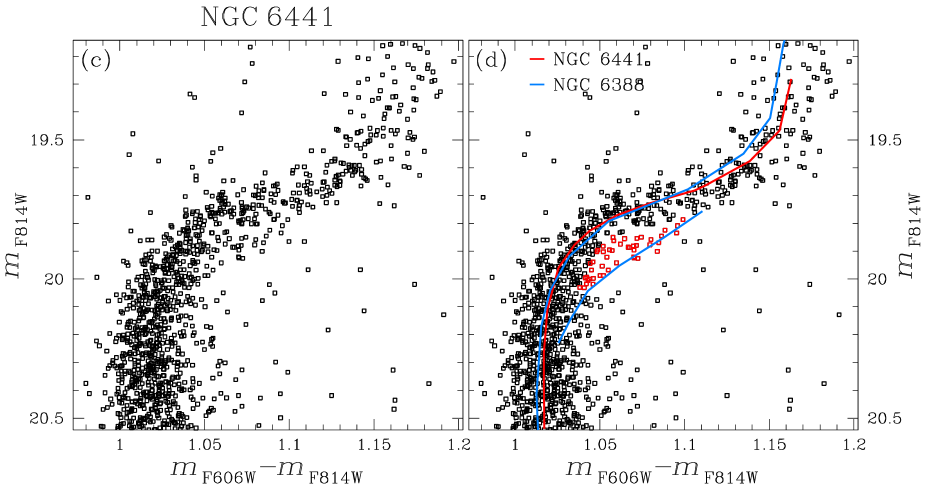
Figure 13: (a) and (b): The SGB region of the CMDs of NGC 6388 (left) and NGC 6441 (right), showing all stars from GO-10775. (c): Proper-motion-selected members of NGC 6441, from the overlap region of GO-10775 and GO-11739. Panel (d) is a replica of panel (c), but with the ridge lines of the MS, the bright part of the SGB, and the lower RGB of NGC 6441 marked in red, and those of NGC 6388 over-plotted in blue—the latter shifted to fit the stars of NGC 6441. The stars that are colored red are the fSGB that is discussed in the text.

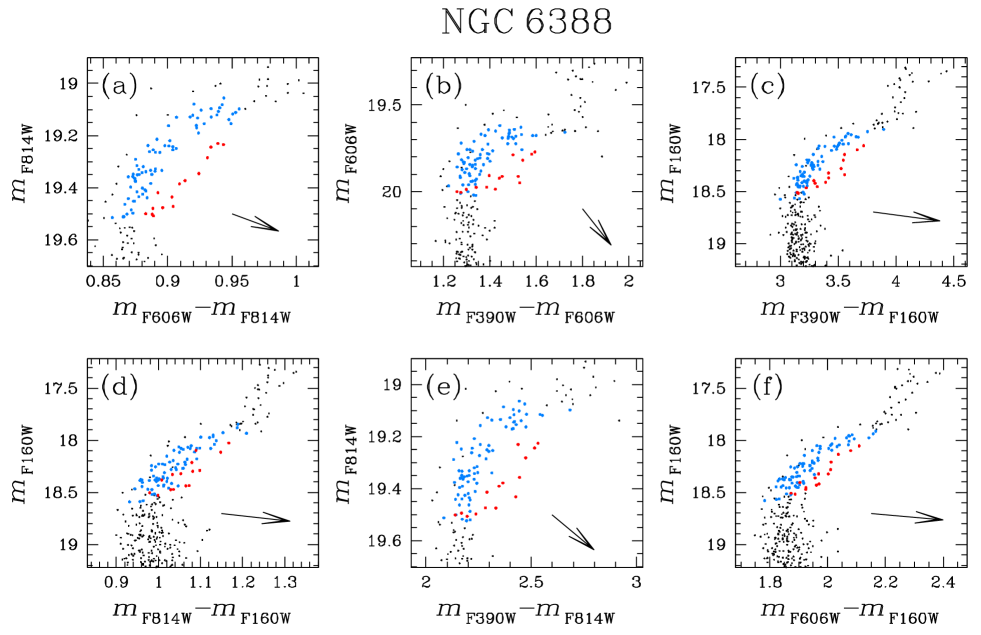
Figure 14: (a): $m_{\rm F814W}$ vs. $m_{\rm F606W}-m_{\rm F814W}$ CMD of the SGB region of NGC 6388 for proper-motion-selected stars in the overlap between GO-10775 and GO-11739, with bSGB and fSGB stars colored azure and red, respectively. The remaining panels show the other color combinations that are available, with each star retaining the color that it was assigned in panel (a). The bSGB and fSGB stars remain well separated in all panels. Reddening vectors are also shown.

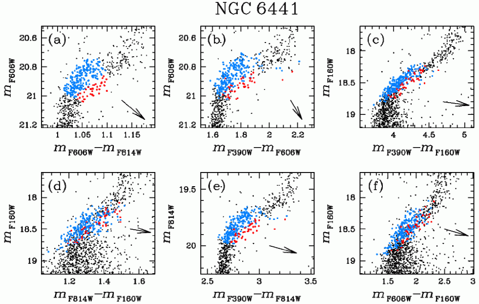
Figure 15: Same as Fig. 14, but for the SGB of NGC 6441. (There are more stars because the overlap between GO-10775 and in GO-11739 is larger for NGC 6441.)

3.4 The Sub-Giant Branches

The top panels of Fig. 13 show the CMDs of NGC 6388 and NGC 6441 around the SGB region in the $m_{\rm F814W}$ vs. $m_{\rm F606W}-m_{\rm F814W}$ plane, both with the same axis scale. All the stars plotted come only from GO-10775. While the SGB split in NGC 6388 is clear, field-star contamination prevents us from analyzing the SGB morphology of NGC 6441 in detail. Nevertheless, it is clear that the overall width of the SGB of NGC 6388 is decidedly larger than that of NGC 6441.

Thanks to the overlap between the fields of view of GO-10775 and GO-11739, we can take advantage of the $\sim$5-year time baseline between the two and use proper motions to isolate probable members of NGC 6441; panel (c) shows the resulting CMD. Now that field-star contamination is no longer an issue, there seems to be a second, fainter and less populated SGB even in NGC 6441 (as could already be suspected in panel (f) of Fig. 6).

Panel (d) is a replica of panel (c) on which we have drawn (in red) the ridge line of the MS, SGB, and RGB as follows. We divided the cluster stars in the figure into 0.15-mag bins (0.4 mag for RGB stars) and derived 3$\sigma$-clipped median values of magnitude and color for each bin. We selected only the brighter SGB for this purpose, while stars that seemed to belong to a fainter SGB have been colored in red. Using the same technique, we derived in a similar way for NGC 6388 the ridge lines for the MS, SGB (both components), and RGB, and drew them in blue. We manually shifted the main-component ridge line of NGC 6388 to best overlap the MS and turn-off regions of NGC 6441.

The SGB split of NGC 6441 is much less than that of NGC 6388. This means that, if a difference in C+N+O is the cause for the SGB split in NGC 6441 and NGC 6388 (as suggested for the case of NGC 1851 by, e.g., Cassisi et al. 2008), that difference must be smaller for NGC 6441 than for NGC 6388.

We performed a multicolor analysis on the SGB region of the clusters. A close-up view of the SGB of NGC 6388 is shown in panel (a) of Fig. 14, for proper-motion-selected stars in common between GO-10775 and GO-11739. The blue and red colors are used to define the bright and the faint SGB components, hereafter bSGB and fSGB, respectively (i.e., in the remaining panels each star will keep the color that it is assigned here). Panels (b) through (f) show the other five CMDs made with the remaining color combinations at our disposal (six total combinations with four filters). The reddening vector is displayed in all panels. Bright and faint SGB stars are color-coded as in panel (a). In all panels the bSGB is brighter than the fSGB, and the two components remain well separated.

Similarly, Fig. 15 shows the multicolor analysis for the SGB of NGC 6441. The bright and faint SGB components for NGC 6441 are selected in the $m_{\rm F606W}$ vs. $m_{\rm F606W}-m_{\rm F814W}$ CMD (panel (a)), and again we plot only proper-motion-selected stars.

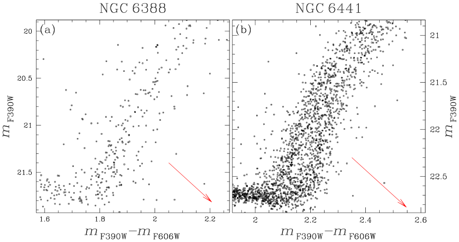
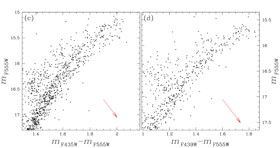
Figure 16: RGBs, plotted on the same scale to facilitate comparison. NGC 6388 is on the left and NGC 6441 on the right. Top and bottom show different color baselines. (F435W and F439W are equivalent filters in two different cameras.) Because the CMDs come from overlap fields of different size, NGC 6388 has fewer stars than NGC 6441 in the top row and more in the bottom row.

Unlike the case of NGC 6388, the two SGB components of NGC 6441 do not remain distinct in all CMDs, but the bSGB stars again stay, on average, brighter than the fSGB stars. The separation of the two groups, however, is much less obvious than for NGC 6388.

A deeper analysis of the SGBs of NGC 6388 and other globular clusters is presented in a separate paper (Piotto et al. 2012).

3.5 The Red-Giant Branches

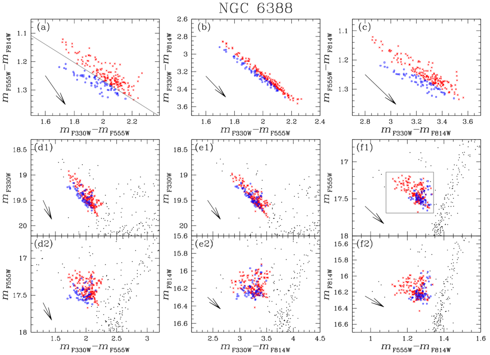
Figure 17: Two-color diagrams (top panels) and CMDs (middle and bottom panels) of the red clump of NGC 6388. The RC sample is defined in panel (f1). The selection of the main and secondary RC components (mRC and sRC, respectively in red and blue) is shown in panel (a).

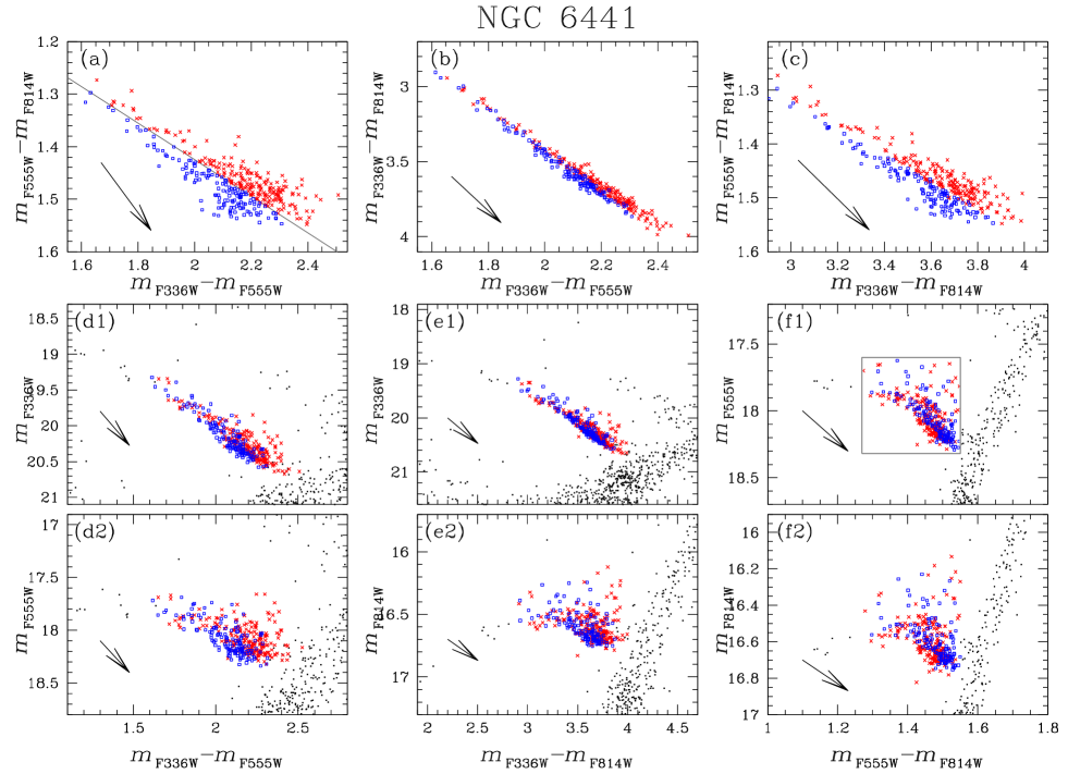
Figure 18: Similar to Fig. 17, but for NGC 6441.

Both NGC 6388 and NGC 6441 have a split RGB, but the splits are different, as shown in Figure 16, in which we see CMDs of the two clusters side by side, with two different color baselines, top and bottom. Unfortunately, in CMDs drawn from quite disparate sources the numbers of stars are not comparable; moreover, the presence of the asymptotic giant branch (AGB) next to the RGB confuses the picture further. Nevertheless, we shall show how to use these CMDs to trace where the brighter and fainter RGB sequences (bRGB and fRGB) run in each cluster.

In panel (c) of Fig. 16 a split in the RGB of NGC 6388 is evident for stars brighter than $m_{\rm F555W}=16.2$. We can exclude the possibility that the brighter RGB sequence might be composed of AGB stars, since the latter are bluer and well separated from the RGB. Panel (a) seems to be suggesting a separation for the entire length of the RGB, but it is hard to draw definite conclusions from so few stars.

For NGC 6441 panel (b) shows a clear split in the faint part of the RGB, but the split becomes less convincing at brighter magnitudes. Panel (d) offers weak confirmation of a split at the bright end, but the star numbers are just too small to be at all sure.

Interestingly, RGB splits are usually found only in ultraviolet photometry (or else in Strömgren filters that are sensitive to molecular bands see, e.g., Gratton et al. 2012, and references therein, for a review); panels (a) and (b) are in agreement with this. By contrast, the cluster M 4, for example, has a very narrow RGB in the $B-I$ color (Marino et al. 2008), but is broad, or even split, in $U-B$. Thus the apparent split of the RGB of NGC 6388 in an optical color (panel (c)) comes as a surprise, and may be suggesting an additional population phenomenon in NGC 6388 and NGC 6441, different from that at work in M 4. Unfortunately, all the stars for which an abundance analysis have been performed (e.g., Carretta et al. (2007), lie at radial distances outside our FoV, and therefore we cannot link a given RGB branch to a particular Na-O family.

In conclusion, the RGBs of these two clusters show evidence of splits, but firmer conclusions await richer samples of stars, or a wider choice of filters, or both.

3.6 The Horizontal Branches

We will focus our HB analysis only on the red clump (RC) region, and not on the extended HB (which is discussed in Section 5.2 instead, in conjunction with the helium abundance).

Milone et al. (2012b) showed that UV two-color diagrams allow a clear separation of the two main populations of 47 Tuc in all evolutionary sequences, and we can profitably use a similar technique on the RC of NGC 6388. Here we chose the small but high-resolution ACS/HRC exposures in F330W, F555W, and F814W. This data set was the best choice we could make. We tried adding F435W from WFPC2 SNAP-9821 for NGC 6388, but it turned out not to add any useful information. We could not combine ACS/HRC with ACS/WFC from GO-10775, because of the severe crowding in the latter. Had we tried instead to use WFC3 F390W exposures, combined with GO-10775, the small spatial overlap would have given too few stars for adequate statistics.

The top row of panels of Fig 17 shows the three possible two-color diagrams from the HRC data set. Panels (d1), (d2), (e1), (e2), and (f1), (f2) show the CMDs of the RC for different color-magnitude combinations.

The choice of red-clump stars that we made is shown by the box in panel (f1). In panel (a) we drew by hand a line that separates the stars into a main and a secondary group (mRC and sRC). The groups are colored red and blue, respectively, and each star retains its color from this panel throughout the rest of the figure.

Panels (a) and (c) clearly show a double-horned RC, a feature that is less obvious in panel (b). We found the sRC to be fainter overall than the mRC (with perhaps the exception of panel (e1)). Moreover, sRC stars are bluer than mRC stars in panels (d1) and (e1), but redder in (f1) and (f2).

Anomalies in the RC morphology have been reported also in the CMDs of NGC 6440 and NGC 6569 by Mauro et al. (2012) and, on a different scale, in the CMD of Terzan 5 by Ferraro et al. (2009), both using IR filters. Since here we instead see the RC split in a two-color diagrams employing UV filters, we think that the cause of the RC split in NGC 6388 is more similar to that of, e.g., 47 Tuc (Milone et al. 2012b), rather than those seen in IR CMDs.

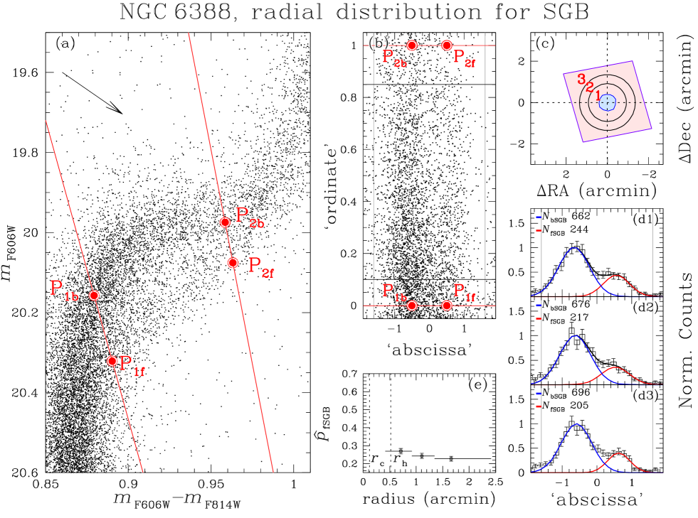
Figure 19: (a) Blow-up of a region of the SGB of NGC 6388, with the four points and two lines marked that are used in the transformation to the coordinate system of the next panel. (See text for details.) (b) Rectification of the SGB region that was shown in (a). The horizontal black lines delimit the ’ordinate’ range used in the analysis, and the vertical gray lines the ’abscissa’ range. (c) The parallelogram is our field. The azure circle is the excluded region in the cluster center; the pink area is the working region that we divided into the three subregions that are marked. (d) Dual-Gaussian fits, in the ‘abscissa’ interval from $-$1.6 to 1.6, of the color distribution of stars in each radial subregion; ‘abscissa’ is the same scale as in (b). Vertical gray lines show the range that was fitted. Black lines are the fits, red and blue lines the individual Gaussians. (e) Relative proportions of the two populations, expressed as the fraction of the total that is contributed by fSGB. Horizontal lines show radial extent of each subregion; error bars come from the sample size and the binomial distribution. Dotted lines mark the core radius and half-light radius.

We performed the same multi-color analysis also for the RC of NGC 6441. To better compare the results between the two clusters, we made use of observations taken through filters as similar as possible to those used for NGC 6388. This choice implied the use of the WFPC2 observations from GO-5667 and GO-8718, which include data collected with the F336W filter instead of the ACS/HRC F330W one. Because of this, results on the RC analysis of NGC 6441 are not one-to-one comparable with those of NGC 6388, but they can still tell us something about similarities or differences between the RC of the two clusters.

Figure 18 is the equivalent of Fig. 17 for NGC 6441. Red-clump stars are again selected in the gray-line box in panel (f1), and stars of the mRC and sRC are again delineated in panel (a) and carry the same colors throughout.

The first difference from the RC of NGC 6388 is that here none of the two-color diagrams has a double-horned shape. In all the CMDs, stars of the mRC and sRC are better mixed than in NGC 6388. In panels (d1) and (d2) sRC stars appear to be bluer (and fainter) than mRC stars. This mRC/sRC dichotomy seems to carry over, although in a less evident way, into panels (e1) and (e2) as well.

The HB regions of these two clusters are at first glance so similar that many investigations (e.g., Rich et al. 1997) lumped the two clusters together; nevertheless, when we look closely the two HBs (in particular their red clumps) are rather different. [Note, however, that the double-horned red clump in NGC 6388 is visible only when the ACS/HRC F330W filter is used. Although the WFPC2 filter F336W throughput is quite similar to that of the ACS/HRC F330W, small differences in filter response may produce quite large effects on the CMD (see, e.g., Momany et al. 2003).] We will resume the discussion of the HBs in Section 5.

4 Radial distributions

NGC 6388 and NGC 6441 have both been revealed to host multiple stellar populations. In this section we will study the radial distributions of these subpopulations, for different CMD regions.

4.1 NGC 6388

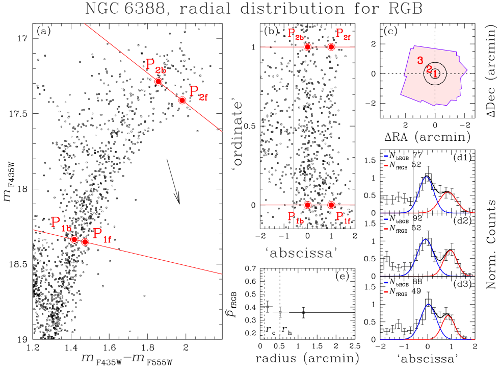
Figure 20: (a) Blow-up of a region of the RGB of NGC 6388, with the four points and two lines marked that are used in the transformation to the coordinate system of panel (b). The analysis makes use only of stars that are to the right of the gray vertical line and between the two red horizontal lines in panel (b). (c) The irregular outline is the total field of view of SNAP-9821, which we used in its entirety, because of the paucity of stars. The three radial zones contain equal numbers of stars. (d) Dual-Gaussian fits of color distribution of stars in each radial subregion; ‘abscissa’ is the same scale as in (b). Black lines are the fits, red and blue lines the individual Gaussians. (e) Relative proportions of the two populations, expressed as the fraction of the total that is contributed by fRGB. Horizontal lines show radial extent of each subregion; error bars come from the sample size and the binomial distribution. Dotted lines mark the core radius and half-light radius.

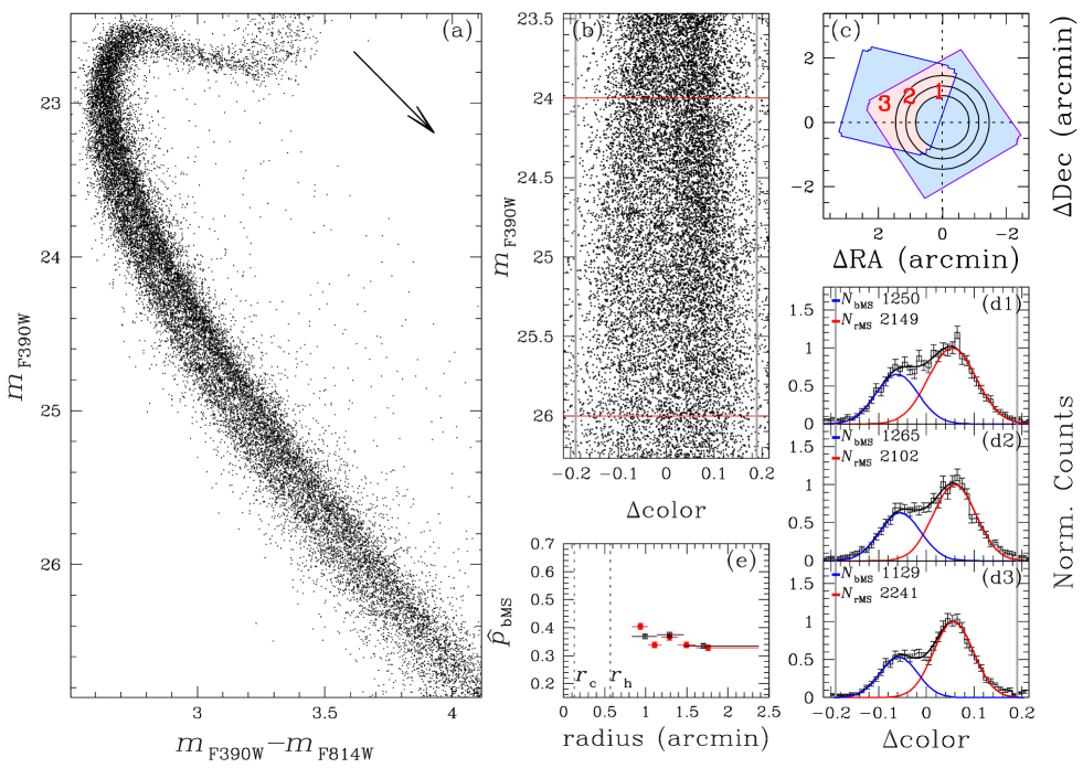
Figure 21: (a) Blow-up of a region of the MS of NGC 6441. For rectification we used the average MS ridge line; the result is shown in panel (b). The stars selected for the analysis are in the region bounded by the red horizontal lines and the gray vertical lines. (c) The footprints of the GO-10775 ACS/WFC images (large parallelogram) and the GO-11739 WFC3/UVIS images (small parallelogram); the pink area is our working region, with our three radial zones marked. (d) Dual-Gaussian fits of color distribution of stars in each radial zone; $\Delta$color has the same scale as (b). Black lines are fits, red and blue lines the individual Gaussians. (e) In black, the fraction of the MS total that is bMS, for the three radial intervals shown in panel (c). Horizontal lines show radial extent of each subregion; error bars come from the sample size and the binomial distribution. The large number of stars allowed a finer radial sampling as an alternative, using five subregions instead of three. Those results are shown in red. Dotted lines mark the core radius and half-light radius.

4.1.1 The Sub-Giant Branch

We started with the double SGB of NGC 6388. We chose to analyze the $m_{\rm F606W}$ vs. $m_{\rm F606W}-m_{\rm F814W}$ CMD of GO-10775 because of the wide separation between the two SGBs in this CMD, and the large number of available stars.

Figure 19 illustrates our analysis of the radial distributions of the SGB components. To rectify the SGB sequence we used a procedure developed by Milone et al. (2009), which we describe here in some detail, as it is rather complicated. First we selected by hand two points ($\rm P_{\rm 1f},P_{\rm 2f}$) on the faint SGB (fSGB) and two points ($\rm P_{\rm 1b},P_{\rm 2b}$) on the bright SGB (bSGB). These points define the two lines in panel (a) of Fig. 19. We then linearly transformed the CMD into a reference frame (which we will refer to simply as ‘abscissa’, ‘ordinate’) in which the origin corresponds to $\rm P_{1b}$ and the coordinates of $\rm P_{1f}$, $\rm P_{2b}$ and $\rm P_{2f}$ are (1,0), (0,1) and (1,1), respectively. (The transformation equation is given in the Appendix of Milone et al. 2009.) This transformation equalizes the separation of the sequences at the two ends of the interval, but they are curved in between the ends. (We do not show this intermediate frame.)

We then used the following procedure to effect a straightening that was a compromise for the two sequences. First we fitted a fiducial line to each of the two sequences, as follows: We divided the bSGB into ‘ordinate’ intervals of 0.025 and the fSGB into intervals of 0.05. For each sequence, within each of these intervals we computed 2.5-$\sigma$-clipped median ‘abscissa’ and ‘ordinate’ values, and then put a smooth spline curve through those points. Then as the line to use for rectification we took a line midway between the smooth spline curves of the two sequences.

The rectification itself consisted of subtracting from the ‘abscissa’ of each star the ‘abscissa’ of this line at the same ‘ordinate’ level. Panel (b) shows the two SGBs rectified in this way. For simplicity, we will refer to the newly obtained $\Delta$‘abscissa’ as just ‘abscissa’. We also show in panel (b) the transformed locations of $\rm P_{\rm 1f}$, $\rm P_{\rm 2f}$, $\rm P_{\rm 1b}$, and $\rm P_{\rm 2b}$.

Stars with ‘abscissa’ between $-$1.6 and 1.6 (gray vertical lines) and ‘ordinate’ between 0.1 and 0.85 (in red) were selected for the radial-distribution analysis.

We excluded from the analysis the innermost 25 arcsec because of high crowding, and divided the remainder of the GO-10775 field into three radial intervals (marked 1, 2 and 3 in panel (c)) in such a way as to have the same number of stars in each interval. The excluded innermost 25 arcsec are colored in azure.

For each radial interval (panels (d1), (d2), and (d3)) we extracted the ‘abscissa’ distribution of the stars within the limits, and did a simultaneous fit of a pair of Gaussians to it, as done in Bellini et al. (2009b). The fit was limited to the ‘abscissa’ values between $-$1.6 and 1.6. The fit is marked with a black curve, while the individual Gaussians for the bright and the faint SGB are colored in blue and red, respectively. In the top-left corner of each of these panels we reported the areas of each of the two Gaussians ($N_{\rm bSGB}$ and $N_{\rm fSGB}$, for the bright and the faint component, respectively).

After this somewhat complicated fitting procedure, it is not immediately obvious how to assign error bars to the numerical ratios of the two components, but the answer becomes clear when we step back and consider what we have done. Our basic aim has been to determine, at each distance from the cluster center, what fraction of the population belongs to each component; the fitting of the dual Gaussians was only a device for estimating how many stars belong to each population component. The statistics of the problem are therefore binomial: if a fraction $p_{\rm fSGB}$ of the stars actually belongs to the fainter component, random samplings from this population will have a binomial distribution, with $\sigma_{N_{\rm fSGB}}=\sqrt{Np(1-p)}$, where $N=N_{\rm fSGB}+N_{\rm bSGB}$ is the sample size. For each observed case, we use as the estimator of the fraction $p$ the quantity $\hat{p}_{\rm fSGB}=N_{\rm fSGB}/N$. Then $\sigma_{\hat{p}_{\rm fSGB}}=\sigma_{N_{\rm fSGB}}/N=\sqrt{\hat{p}_{\rm fSGB}(1-\hat{p}_{\rm fSGB})/N}$; this is our best estimate of the error bar of $\hat{p}$.

That is what we have done. One should bear in mind, however, that in so far as our estimation methods might be somewhat imperfect, the true uncertainty could be somewhat larger than this error bar. (We prefer to make this simple statement, rather than attempt to doctor the statistics.)

In panel (e) we summarize the results of the analysis: values of $\hat{p}_{\rm fSGB}$ are plotted as a function of the median radial distance of the stars in each radial interval, with errors. The horizontal lines show the radial range to which each point applies. Vertical dashed lines mark the core radius $r_{\rm c}$ and the half-light radius $r_{\rm h}$. We ran artificial-star experiments to check for possible influence of incompleteness on the radial gradients. We found that in the radial interval covered by our images the completeness is always higher than 84%, with marginal differences (at most 2%) between bSGB and fSGB stars. Therefore incompleteness cannot significantly change the results displayed in Fig. 19.

We notice some marginal evidence of a gradient, with fSGB stars more concentrated than bSGB ones.

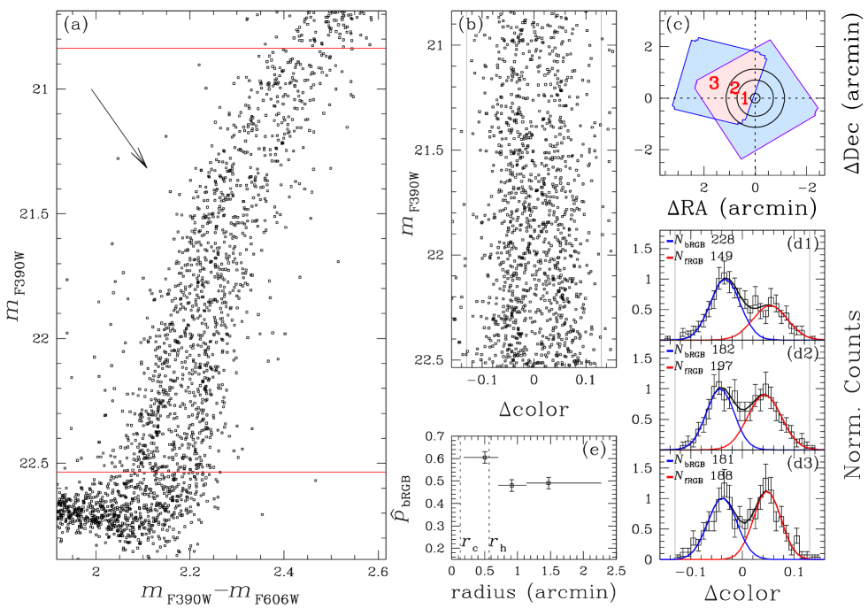
Figure 22: As in Fig. 21, but for the RGB sub-populations of NGC 6441.

4.1.2 The Red-Giant Branch

To study the radial distributions of the RGB of NGC 6388 we chose the ACS/WFC F435W–F555W CMD of SNAP-9821, the data set that was able to split the RGB in Fig. 16.

In panel (a) of Figure 20 we see the bRGB and fRGB (as we again call the two components) well separated at the brighter end but badly blended at fainter magnitudes — a situation for which our dual-Gaussian technique is well suited.

We began with a transformation and rectification procedure like the one that we described for the SGB. This case was a little easier, because the two population branches turned out to be parallel after the transformation, so that fewer steps were required for the rectification.

A glance at panel (b) reveals a serious problem, however: the encroachment of the AGB on the bRGB. (We purposely show a wide range of ‘abscissa’ so as to expose this issue.) Because of the AGB, the bluest range of ‘abscissa’ will have to be “out of bounds” for our fitting of the Gaussians, with a cut-off not far to the left of the peak of the Gaussian that fits the bSGB. The placement of the cutoff is then a delicate question, to answer which we invent a special procedure. Without any question of radial binning yet, we analyze all the stars that are between ‘ordinate’ values 0 and 1 in panel (b). We make use of the fact that the number of AGB stars is a very different function of ‘ordinate’ from the number of RGB stars. As a criterion for absence of AGB interference, we divide the ‘ordinate’ range from 0 to 1 into three separate parts, and require that the ratio $N_{\rm fRGB}$/$N_{\rm bRGB}$, as derived from our dual-Gaussian fitting with the lowest values of ‘abscissa’ excluded, come out the same for all three ranges of ‘ordinate’. We carry out this test (which is not illustrated here) for various placements of the cut-off, and choose the cut-off that is farthest to the left but still satisfies the criterion. That value is the vertical gray line in panel (b).

(A thoughtful reader may ask how we can be sure that the two populations represented by the bRGB and the fRGB should have the same distribution of stars with ‘ordinate’ value. The answer is that this distribution is set by gross rules of stellar structure, as a star moves up the RGB; these rules are quite insensitive to the small differences that separate these two populations. AGB evolution is governed by quite different physics, however, and leads to a very different distribution of ‘ordinate’ values.)

With this problem disposed of, we can proceed to the selection of radial bins. Crowding is not an issue for these bright stars; we can study them even in the very core of the cluster. Farther from the center, however, the star numbers become too small. In panel (c) the azure outline is our SNAP-9821 field, and the region that we studied is in pink.

We had found the best ‘abcissa’ interval to have its left limit at $-0.6$, which is marked with a gray vertical line in panels (d1), (d2), and (d3). (We show the full ‘abscissa’ range of panel (b), however.) The best-fit dual Gaussians are shown in each of the panels (d), in blue and red for the bright and the faint RGB component, respectively. We also show the areas of the Gaussians (i.e., star numbers) in the top-left corner.

Finally, in panel (e) we report $\hat{p}_{\rm fRGB}=N_{\rm fRGB}/(N_{\rm fRGB}+N_{\rm bRGB})$ as a function of the median distance of the stars from the cluster center in each radial interval, with error bars calculated as explained in the previous subsection.

There is no evidence for a radial gradient, though it must be noted that the error bars are much larger than in the previous case, because of the smaller number statistics.

4.1.3 A possible relation between the radial distributions of the SGB and the RGB

The radial distribution of $\hat{p}_{\rm fSGB}$ extends from the half-light radius, at $0\farcm 5$, out to $\sim 2\farcm 4$; our results give marginal evidence of a decrease (at $\sim$2$\sigma$). Our RGB analysis is extended to larger radii $r<2\farcm 65$, but with a much smaller number of stars and, for what it its worth, no evidence for a radial gradient in the population fractions. In both cases one component (bSGB or bRGB) is significantly more numerous than the other. It is tempting to consider the bRGB as the progeny of the bSGB, although $\hat{p}_{\rm fRGB}$ is larger than the inward extrapolation of $\hat{p}_{\rm fSGB}$. We will discuss possible implications of these results in the final section.

4.2 NGC 6441

4.2.1 The Main Sequence

We have seen that NGC 6441 hosts two distinct stellar populations, clearly detectable both on the MS and on the RGB (whereas for NGC 6388 the separations were on the SGB and RGB).

To measure the population fraction of the two MSs we again used the dual-Gaussian fitting technique. Panel (a) of Fig. 21 shows a close-up of the MS of NGC 6441 in the $m_{\rm F390W}$ vs. $m_{\rm F390W}-m_{\rm F814W}$ CMD, chosen because this combination of filters enhances the split of the MSs. We computed the MS ridge line as done in subsection 4.1.1 for the SGBs of NGC 6388, then we subtracted from the color of each star the color of the ridge line at the same magnitude as the star. The rectified MS ($\Delta$color) is plotted in panel (b), in the magnitude interval $23.05<m_{\rm F390W}<27.05$. Stars with $24<m_{\rm F390W}<26$ (red horizontal lines) and $\Delta$color between $-$0.19 and 0.19 (gray vertical lines) were used for the radial-distribution analysis.

Panel (c) shows the footprints of GO-10775 and GO-11739 (larger and smaller parallelograms, respectively). The overlap region used for the analysis is colored pink. We excluded the centermost 50 arcsec because of crowding problems. As done for the other radial-distribution analyses, we defined three radial bins, each containing the same number of selected stars.

Panels (d1), (d2), and (d3) show the histograms of the $\Delta$color distribution within each radial interval. The best-fit dual Gaussians are shown in blue and red for the bMS and the rMS, respectively. The areas of the Gaussians are also shown, as done in Figs. 19 and 20, in the top-left of each (d) panel. The ‘abscissa’ interval used to fit the dual Gaussian is marked with gray vertical lines.

For each radial interval we derived the values of $\hat{p}_{\rm bMS}=N_{\rm bMS}/(N_{\rm bMS}+N_{\rm rMS})$, with errors, which are in black in panel (e). Motivated by the fact that there are more than 3000 stars in each radial interval, we decided also to derive a finer sampling of the radial distribution of $\hat{p}_{\rm bMS}$. Therefore, we divided the pink area in panel (c) into five equally populated radial intervals. For each of them we fitted a dual Gaussian (not shown) and computed $\hat{p}_{\rm bMS}$ values, which are reported, in red with errorbars, in panel (e). There is strong evidence of a radial gradient, with the bMS more concentrated than the rMS.

4.2.2 The Red Giant Branch

Finally, we analyzed the radial distribution of the two RGB components of NGC 6441. A close-up view of the RGBs in the $m_{\rm F390W}$ vs. $m_{\rm F390W}-m_{\rm F606W}$ CMD is shown in panel (a) of Fig. 22. To rectify the sequences, we derived a fiducial line for the whole RGB, and subtracted from the color of each star the color of the fiducial line at the same magnitude level. The rectified RGB is shown in panel (b). For the radial-distribution analysis we selected stars in the magnitude range $22.52\leq m_{\rm F390W}\leq 20.84$ (red horizontal lines in panel (a)), and between $\Delta$color $-$0.13 and 0.13 (gray vertical lines in panel (b)).

Since we are using the same data set as for the MS of NGC 6441, panel (c) shows the same footprints as Fig. 21c. We excluded the centermost 11.1 arcsec because of crowding, and defined three radial intervals, each containing the same number of stars.

In panels (d1), (d2), and (d3) we show the histograms of the $\Delta$color distributions for the three radial intervals, together with the best-fit Gaussians and their areas. In blue we mark the bRGB component, in red the fRGB one, and the combined curve is in black.

For each radial interval, we computed $\hat{p}_{\rm bRGB}=N_{\rm bRGB}/(N_{\rm bRGB}+N_{\rm rRGB})$ along with its error, and plotted these as a function of median radial distance, in panel (e).

As for the MS, there is some evidence of a radial gradient, with the bRGB more concentrated than the rRGB. Analogously with the SGB and RGB of NGC 6388, the similarity in radial gradients here is consistent with the populations of the RGB of NGC 6441 being the progeny of those of the MS – although here again there is a disagreement in the mean numbers.

4.2.3 A possible relation between the radial distributions of the SGB and the RGB

In summary, our values of $\hat{p}_{\rm bMS}$ extend from $\sim$$0\farcm 8$ (inside of which the crowding is too great) out to $\sim$$2\farcm 4$; in this range, the number of bMS stars relative to the rMS shows a significant outward decrease. Similarly, our study of the RGB showed an outward decrease of the number of bRGB stars relative to fRGB. However, as in the case of SGB and RGB stars in NGC 6388, here too there is an inconsistency between the overall levels of $\hat{p}_{\rm bMS}$ and $\hat{p}_{\rm bRGB}$. We will discuss the implications of these results in the final section.

Table 3
Results of Radial Distribution Analyses for NGC 6388
SGB				RGB
$r_{\rm med}$ $(^{\prime})$	$N$	$\hat{p}_{\rm fSGB}$	$\sigma_{\hat{p}_{\rm fSGB}}$	$r_{\rm med}$ $(^{\prime})$	$N$	$\hat{p}_{\rm fRGB}$	$\sigma_{\hat{p}_{\rm fRGB}}$
0.711	906	0.269	0.015	0.195	129	0.403	0.043
1.108	893	0.243	0.014	0.529	144	0.361	0.040
1.661	901	0.228	0.014	1.141	137	0.358	0.041

4.3 Population ratios and their radial gradients

In this section we summarize the results illustrated in Figures 19–22, concerning the number ratios between the two populations, and the radial gradients of the ratios. In the outer regions of NGC 6441 (outside $\sim$$0\farcm 8$), the blue MS represents $\sim$1/3 of the total population ($\hat{p}_{\rm bMS}$$\sim 0.33$), with a small radial gradient; closer to the center the crowding prevents us from distinguishing the two MSs. For the RGB we can reach the cluster center, where the fRGB actually predominates by a little, with a radial gradient bringing $\hat{p}_{\rm fRGB}$ below 0.5 farther out. Unfortunately, radial gradients make it difficult to compare population ratios for different evolutionary sequences, but it does look, at first sight, as if: (i) the CMD locus of the bMS population crosses through the locus of the rMS population; (ii) the two SGBs overlap, and it is difficult to say whether the bMS population joins the bRGB or the fRGB. For NGC 6388 we could not split the MS, so the population ratio and its radial trend were derived only for the SGB and the RGB — complicating comparisons, by leaving us with MS and RGB for NGC 6441, but SGB and RGB for NGC 6388.

The results for the two clusters are summarized in Tables 3 and 4, respectively, which give the median radius of each zone, the number of stars in the zone, the fraction that belong to the fainter component (or in the case of the MS, to the bluer branch), and the statistical uncertainty of the fraction. Alternatively, the same results can be viewed graphically in the (e) panels of Figures 19–22.

The overall tendency is to have one sequence more concentrated towards the cluster center, although this is not always statistically significant. In particular, for NGC 6441 both bMS and bRGB are more centrally concentrated, and the latter can be considered the progeny of the former. For NGC 6388, instead, while the fSGB population is more centrally concentrated, the distribution of the two populations in the RGB region is found to be flat. Based solely on star counts, we can tentatively consider bRGB as the progeny of bSGB, each being the more populated branch.

Table 4
Results of Radial Distribution Analyses for NGC 6441
MS				RGB
$r_{\rm med}$ $(^{\prime})$	$N$	$\hat{p}_{\rm bMS}$	$\sigma_{\hat{p}_{\rm bMS}}$	$r_{\rm med}$ $(^{\prime})$	$N$	$\hat{p}_{\rm bRGB}$	$\sigma_{\hat{p}_{\rm bRGB}}$
0.993	3399	0.368	0.008	0.505	377	0.605	0.025
1.290	3367	0.376	0.008	0.914	379	0.480	0.026
1.703	3370	0.335	0.008	1.472	369	0.491	0.026
0.936	2089	0.404	0.011
1.108	2087	0.338	0.010
1.289	2088	0.366	0.011
1.496	2088	0.338	0.010
1.757	2089	0.328	0.010

Table 5
Statistical Analysis of the Radial Gradients
Fig.	NGC	component	$N$	$A$	$\sigma$	signif
19	6388	fSGB	3	$-$0.042	0.021	1.95
20	6388	fRGB	3	$-$0.041	0.062	0.67
21	6441	bMS	3	$-$0.050	0.016	3.14
21	6441	bMS	5	$-$0.069	0.016	4.31
22	6441	bRGB	3	$-$0.112	0.037	3.01

Table 6
Multipopulation Summary
sequence	NGC 6388	NGC 6441
MS	broadened	split
SGB	split	hints of a split
RGB	split	split
HB (red clump)	split	broadened

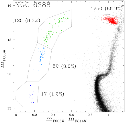
ppp

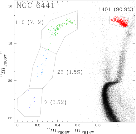
Figure 23: The horizontal-branches of NGC 6388 and NGC 6441 in the $m_{\rm F606W}$ vs. $m_{\rm F606W}-m_{\rm F814W}$ CMD. We identified by hand four regions, colored in red for the RC, and green, azure, and blue for three distinct segments of the blue HB, from brightest to faintest. Internal labels give the number of stars in each of these regions, and the fraction of the total HB population that it constitutes.

In the study of the population ratios listed in Tables 3 and 4, it is important to judge whether apparent radial gradients are real or not. To test this, we calculated a least-squares line through each set of points. With at most five observed points, any formal error for the slope of the line would be meaningless, so we instead made a Monte Carlo simulation. In place of each observed point we took a Gaussian with mean equal to the value of the point, and with the sigma of the point, and we calculated the slope $A$ for each of a million random samplings from these Gaussians. The million values of $A$ had a distribution that was closely Gaussian; Table 5 gives the resulting slopes (per arcmin) and their sigmas. In the last column of the table is the ratio of $|A|$ to $\sigma$, which is an index of how reliably a slope differs from zero; a $2\sigma$ result is of course only marginal, while a $3\sigma$ result is quite significant. Thus the radial gradient in Fig. 19 is marginal, that in Fig. 20 dubious, and those in Figs. 21 and 22 highly significant.

5 Discussion

5.1 Summary of the observational evidence of multiple stellar populations

We have analyzed a large sample of proprietary (GO-11739) and archival images of the two massive, metal-rich Galactic-bulge GCs NGC 6388 and NGC 6441, have used proper motions to remove most of the field stars, have corrected all our CMDs for differential reddening, and have made a thorough multicolor analysis of the stellar populations of the two clusters.

In both clusters we found significant evidence for the presence of at least two stellar generations, which manifest themselves as broadened or multiple sequences in all the main evolutionary branches of the CMDs. Table 6 collects the main results on the multiplicity of the various sequences. These results are distilled from a quite complex data set, whose most important aspects are summarized next.

The MS of NGC 6388 is analyzed with various filter combinations in Figs. 9–11. Most of the CMDs show a broadening of the MS, but none of them succeeds in splitting it into distinct sequences as instead happens for NGC 6441 when using the $m_{\rm F390W}-m_{\rm F814W}$ color, as shown in Figures  6(g) and 21. The separation of the two MSs of this latter cluster as a function of color baseline is illustrated in Fig. 12 Figure 8 further confirms the reality of these results for both clusters, showing that neither of them could result from differential reddening (for which all CMDs have been corrected). Note, moreover, that the average reddening of NGC 6388 is lower than that of NGC 6441 (see subsection 2.5), hence it should have been easier to recognize two MSs (if present) compared to the case of NGC 6441. We conclude that the MS structures of the two clusters are different.

The SGBs of the two clusters are examined in Fig. 13 which shows a clear split for the SGB of NGC 6388 in panel (a) but at best a doubtful one for NGC 6441 in panels (c) and (d), where the SGB components apparently overlap; Figures 14 and 15, respectively, explore the SGB for each cluster in multicolor domains. Again, we note this more subtle difference between the two clusters, with two distinct SGBs in NGC 6388 and just a broadened SGB in NGC 6441 (the opposite situation compared to the MS).

The structure of the RGB of the two clusters is shown in Fig. 16. In both cases there is a hint of a double RGB, more evident in the upper part of the RGB of NGC 6388 and in the lower part for NGC 6441. The evolutionary connection between the MS and the RGB is somewhat ambiguous in the case of NGC 6441: the population ratio seems to indicate that bMS and fRGB stars belong to the same population, but the radial gradient (which complicates the calculation of the population ratios) suggests instead to connect the bMS to the bRGB. For NGC 6388 it appears that bSGB and bRGB stars belong to the same population.

For the HB we have thus far examined only the red clump; we take up the extended blue part of the HB in the following. The split of the RC of NGC 6388 can be seen in the two-color diagrams in panels (a) and (c) of Fig. 17, while for NGC 6441 the broadening is seen in most of the panels of Fig. 18. Therefore there is some evidence that the RC is also a mixture of the first and second generations. However, what makes these two clusters unique, among the 150 globular clusters of the Milky Way, is their blue HB extension in spite of their high metallicity. Furthermore, their blue HBs are remarkably similar, as illustrated in Fig. 23. Note also the similarity of the relative number of stars in the distinct sections into which we have divided the HB. This similarity is particularly surprising given that — as is well known — the distribution of stars on the HB is extremely sensitive to many different parameters (age, composition, RGB mass loss). Thus, the differences in the structure of the MS, SGB and RGB of the two clusters demonstrate that there must be a sizable difference in some of those parameters, and yet the HBs turn out to be very similar. This conundrum is further discussed in the last subsection.

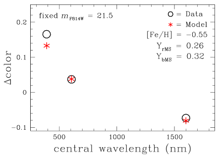
Figure 24: Points from panel (d) of Fig. 12, on which we have superimposed values of $\Delta$color that follow from synthetic colors calculated with our best-fit value of the helium abundance of the bMS of NGC 6441.

5.2 The helium abundance of the secondary populations

Photometric differences in the CMD between multiple stellar populations in GCs have been attributed to differences in helium (e.g., Bedin et al. 2004; Norris 2004; D’Antona et al. 2005; Piotto et al. 2005, 2007) or in light-element abundances (e.g., Sbordone et al. 2011). Different photometric bands can enhance different effects of the chemical pattern of the population. As noted in the introduction, the presence of helium-enriched stars in these two clusters was first proposed based on the exceptional morphology of their HBs and on the properties of their RR Lyrae variables. Now, the discovery of a double main sequence in NGC 6441 lends support to this interpretation, and favors a scenario in which the helium-rich stars belong to a second stellar generation, as opposed to the possibility that they would owe high helium to deep-mixing on the upper RGB, as proposed by Sweigart & Catelan (1998).

Our studies of 47 Tuc (Milone et al. 2012b), NGC 6397 (Milone et al. 2012c), and NGC 6752 (Milone et al. 2010) demonstrate that light-element variations should not significantly affect the $m_{\rm F606W}-m_{\rm F814W}$ or $m_{\rm F814W}-m_{\rm F160W}$ colors of MS stars, so we explore the possibility of helium being the chief cause of the observed MS split in NGC 6441 (or of MS broadening, depending on the specific bands). To this end, we calculated synthetic colors for the two MSs, adopting a primordial helium $Y$=0.26 for the rMS, while trying for the bMS $Y$ values between 0.27 and 0.36, in steps of 0.01. We assumed for each sub-population the same iron abundance ([Fe/H]=$-$0.55 Harris 1996, 2010 edition, see also Carretta et al. 2009b, Origlia et al. 2008). Note that a difference of 0.1 dex in [Fe/H] (which represents the present uncertainty in the metallicity difference between the two clusters) in the calculated models does not change our conclusions.

In previous papers we have used a similar approach to estimate helium differences between GC sub-populations, but there we knew the light-element abundance of the two MSs and here we do not. Hence, we assume the abundance of C, N and O to be the same, in spite of likely differences in at least their relative proportions between the first and second generations. In practice, we assumed [C/Fe]=$-$0.45, [O/Fe]=0.27 (Origlia et al. 2008), and solar N abundance. In both cases we used [$\alpha$/Fe]=0.3 (Origlia et al. 2008). Neglecting possible differences of CNO proportions should not affect our conclusion about helium because, as noted above, the F606W, F814W and F160W filter bands are almost completely insensitive to C, N, and O, while only F390W is expected to be somewhat affected by abundance variations in these light-elements.

We adopted the synthetic colors from the BaSTI isochrones (Pietrinferni et al. 2004) in order to compare observations and synthetic colors, and determined $T_{\rm eff}$ and $\log g$ for MS stars at $m_{\rm F814W}$=21.5. The ATLAS12 code (Kurucz 2005; Castelli 2005; Sbordone et al. 2007) was then used, which allows us to work with arbitrary chemical compositions. We performed spectral syntheses from 3,400 Å to 20,000 Å by using the SYNTHE code (Kurucz 2005), and integrated the synthetic spectra over the transmission curves of the four filters. From the resulting fluxes we formed, for each value of $Y$, the differences $\Delta{\rm color}=m_{\rm X}-m_{\rm F814W}$.

Our result is shown in Fig. 24. We found that the value $Y_{\rm bMS}$=0.32 optimizes the agreement between models and observations. The overall good agreement suggests that helium can indeed be the main cause of the observed split, with bMS stars being He-enhanced by $\Delta Y$$\sim$0.06 relative to rMS stars. Best-fit model and data are less in agreement for the F390W point, as expected because this band-pass includes CN and CH molecular bands, hence the flux through this band is sensitive to CNO variations (e.g., Milone et al. 2012b).

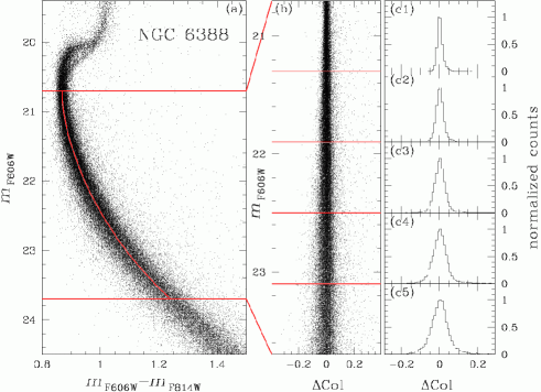
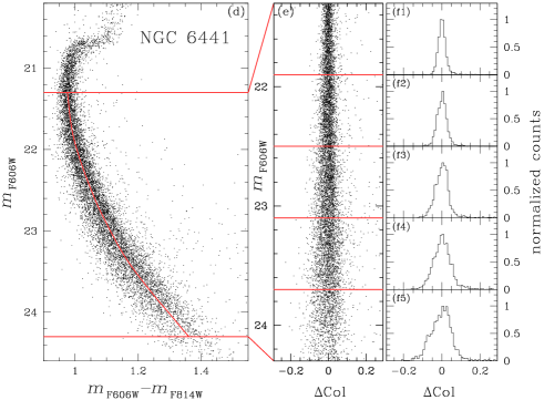
Figure 25: Illustration of the procedures used to determine the MS intrinsic breadth of the two clusters in $m_{\rm F606W}-m_{\rm F814W}$. Panels (a), (b), and (c) refer to NGC 6388, Panels (d), (e), and (f) to NGC 6441. See text for details.

In the case of NGC 6388 there is no evidence of a split in its MS, which is clearly broader than expected from photometric errors, but the color spread (in $m_{\rm F390W}-m_{\rm F814W}$) is smaller than that of NGC 6441. However, as previously emphasized, the $m_{\rm F606W}-m_{\rm F814W}$ color baseline is more sensitive to helium variation, but is insensitive to variations of CNO. In Figure 25 we compare the $m_{\rm F606W}$ vs. $m_{\rm F606W}-m_{\rm F814W}$ CMDs of NGC 6388 and NGC 6441. Panels (a) and (d) are the CMDs themselves (from the overlapping regions of GO-11739 and GO-10775, proper-motion-selected members only for NGC 6441). Panels (b) and (e) show the rectified MSs, extending $\sim$3 magnitudes below the TO. The rectified $\Delta$color distribution, in five magnitude intervals, is shown in panels (c) and (f).

The color distributions appear to be symmetric in NGC 6388 but slightly skewed bluewards in NGC 6441. Table 7 gives the MS breadths, from fitting Gaussians to the distribution of $\Delta$color. The first column identifies the panel in the figure, and the final column gives the intrinsic breadths, calculated as the quadrature difference between the preceding two columns. These breadths are also plotted in Fig. 26 as a function of the $m_{\rm F606W}-m_{\rm F606W}^{\rm TO}$ magnitude. We conclude that the intrinsic $m_{\rm F606W}-m_{\rm F814W}$ color dispersions of the two MSs are quite similar, so that despite the different manifestation of the two populations, at least their helium distributions must likewise be quite similar.

Though a complete and thorough analysis and interpretation of the numerous CMDs presented here is deferred to a future paper (Cassisi et al. in preparation), we wish to present here some further remarks on the estimates of the helium abundance in the stellar populations of NGC 6388 and NGC 6441.

The $Y$$\sim$0.32 that we found for the bMS stars in NGC 6441 from the MS separations in the various color baselines can be compared with the He content estimated by Caloi and D’Antona (2007) and by Busso et al. (2007) from their analysis of the HB morphology and of the pulsational properties of the RR Lyrae stars in this cluster. Busso et al. were able to reproduce the blue and tilted HB morphology of NGC 6441 by assuming a He abundance $Y$$\approx$0.35 for the second-generation stars, only $\sim$0.03 higher than our estimate from the MS split. At the same time Caloi & D’Antona suggested that a fraction of the NGC 6441 stars would have a He content as high as $Y$=0.38–0.40 in order to account for the extreme blue part of the HB. Part of this discrepancy with our present result and that of Busso et al. could be due to the use of optical bands by Caloi & D’Antona, which surely are not optimal for studying the very hot HB extension (see Dalessandro et al. 2011). Moreover, in order to match synthetic to observed HBs, both Busso et al. and Caloi & D’Antona appeal to a substantial spread of helium from $Y$$\simeq$0.25 in the first generation up to the their maximum estimated values (0.35 and 0.40, respectively). Our result, with two distinct MSs in NGC 6441 suggests instead that (at least in this cluster) there are basically two distinct values of the helium abundance, with a clear gap in between.

Furthermore, there is yet another puzzling inconsistency between the results of those two investigations based on the HB and the results of the present paper. According to Caloi & D’Antona only $\sim$38% of the stars in NGC 6441 would have primordial He content ($Y\sim$0.25), whereas according to Busso et al. only 15–16% of the stars should belong to the second generation. Though in different ways, both results are at variance with what we obtained from the two MSs of this cluster, i.e., the majority of stars ($\sim 65$%) are on the red (presumably first-generation) MS and only $\sim 1/3$ appear to belong to the second generation. We shall come back to this issue in the next subsection.

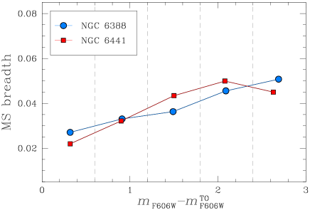
Figure 26: MS breadth in $m_{\rm F606W}-m_{\rm F814W}$ as a function of the magnitude $m_{\rm F606W}$ below the TO. Blue for NGC 6388, red for NGC 6441.

Table 7
Intrinsic MS Breadth in $m_{\rm F606W}-m_{\rm F814W}$ Colors
Ref.	$N_{\rm stars}$	$\langle m_{\rm F606W}\rangle$	$\Delta$Col rms	$\sigma$	Breadth
NGC 6388
(c1)	10148	21.02	0.015	0.031	0.027
(c2)	12109	21.61	0.018	0.038	0.033
(c3)	12119	22.19	0.023	0.043	0.036
(c4)	10801	22.79	0.030	0.054	0.046
(c5)	8987	23.39	0.041	0.065	0.051
NGC 6441
(f1)	1626	21.62	0.016	0.027	0.022
(f2)	1935	22.20	0.021	0.038	0.032
(f3)	2048	22.80	0.028	0.051	0.043
(f4)	1947	23.38	0.037	0.062	0.050
(f5)	1134	23.93	0.052	0.069	0.045

At least part of these discrepancies can be traced to the assumption made by Busso et al. that the whole red clump consists of first-generation stars, with second-generation stars confined to the blue HB extension; indeed, the RC represents $\sim$12–15% of the total HB population. We have found instead that the RC is a mixture of first- and second-generation stars. It is then possible that all second-generation stars arrive on the HB at the RC, spend there roughly 50% of the HB lifetime, and then evolve into an extended blue loop for the remaining $\sim$50% of the time. In fact, as emphasized by Caloi & D’Antona, the evolution of the helium-rich and metal-rich HB models may be confined to the RC region, or, after spending some time on the RC, the stars may experience an extended excursion reaching very blue colors for differences in total mass of order of just $\sim 0.01\,M_{\odot}$ (Sweigart & Gross 1978). For this reason, it is difficult to precisely pinpoint the helium abundance from the mere extension of the HB.

Finally, we note that the MS breadth in the $m_{\rm F606W}-m_{\rm F814W}$ color increases with decreasing luminosity (see Fig. 26 and Table 7) in a fashion that apparently cannot be accounted for by the increasing photometric errors. Here, we simply observe that an increase of the MS spread in the 2–3 magnitude interval below the TO is also observed in the MSs of $\omega$ Cen (King et al. 2012) and NGC 2808 (Piotto et al. 2007). We shall return on this observational evidence in a future paper.

5.3 An NGC 6388–NGC 6441 conundrum?

As already emphasized, these two clusters are unique in having a major blue horizontal branch extension in spite of their high metallicity and in the properties of their RR Lyrae variables. Furthermore, their HBs are remarkably similar in shape and extension and even in the relative star numbers along the branches (see Fig. 23). The two clusters also have in common the presence of two population components whose distinctness is evident in various parts of their CMDs, with the population that is (slightly) more concentrated to the center likely being the second generation. The outstanding anomaly, however, is that whereas the MS of NGC 6441 is clearly split into two branches (in $m_{\rm F390W}-m_{\rm F814W}$ color), that of NGC 6388 is single, though broadened. Given the extremely high sensitivity of the HB morphology to the helium abundance, we conclude that the helium difference between the two stellar generations must be similar, in the two clusters. The results presented in Fig. 25 and 26, showing the close similarity of the MS of the two clusters in the $m_{\rm F606W}-m_{\rm F814W}$ color, strengthen this conclusion further. How can these clusters exhibit almost identical HBs while having very different MS properties in $m_{\rm F390W}-m_{\rm F814W}$ color? In other words, if the second generation populations in the two clusters have nearly identical helium abundances, why is the MS split in NGC 6441 but not in NGC 6388? Clearly, something else must differ in order to reduce below detection the MS split of NGC 6388, or to amplify that of NGC 6441. This is the conundrum of what is otherwise a pair of twin clusters.

One possibility is metallicity [Fe/H], such that in NGC 6388 the helium-rich population is also somewhat metal-enriched, while it is not in NGC 6441. This possibility appears to be excluded by the high-resolution spectroscopy of Carretta et al. (2007), according to which RGB stars in NGC 6388 have the same [Fe/H] within $\sim$0.01 dex. Their sample consists of just seven stars, however, so that the chance of their having missed the minority population is not entirely negligible. However, among these seven stars there appears to be a spread in oxygen, sodium, and aluminum abundances, which should indicate that, though small, the sample actually includes stars from both the first and the second generation. This is confirmed also by a lower-resolution study of a larger sample of stars (Carretta et al. 2009a). The option that the seven stars of Carretta et al. all belonged to a single population does not appear to be supported by observations.

As emphasized above, the main difference between the two clusters arises when the F390W filter comes into play, and within its passband strong CN and CH bands are included (see Fig. 32 in Milone et al. 2012b). A more attractive option is therefore that the secondary population in NGC 6388 is CNO-enhanced compared with the first generation, though this requires a chemical enrichment scenario that is quite ad hoc. In this way excess CN and/or CH molecular blanketing in the UV would make redder the MS of the secondary population in this cluster. A similar effect could also be produced by the C:N:O proportions in the secondary population of NGC 6388 being different from those in the secondary population of NGC 6441.

We defer to a future paper a more quantitative exploration of these alternatives (Cassisi et al., in preparation), but we note that further progress will require an extensive spectroscopic exploration of these clusters at high spectral resolution, in particular having photometrically identified the targets as belonging to one or the other sub-population. More extensive HST observations, especially at ultraviolet wavelengths, would also help in solving this conundrum.

References

- (1) Anderson, J., & King, I. R. 2000, PASP, 112, 1360
- (2) Anderson, J., & King, I. R. 2006, ACS/ISR 2004-15 (Baltimore: STScI) (2006a)
- (3) Anderson, J., & King, I. R. 2006, ACS/ISR 2006-01 (Baltimore: STScI) (2006b)
- (4) Anderson, J., Bedin, L. R., Piotto, G., Yadav, R. S., & Bellini, A. 2006, A&A, 454, 1029
- (5) Anderson, J. 2007, ACS/ISR 2007-08 (Baltimore: STScI)
- (6) Anderson, J. et al. 2008, AJ, 135, 2055
- Anderson et al. (2009) Anderson, J., Piotto, G., King, I. R., Bedin, L. R., & Guhathakurta, P. 2009, ApJ, 697, L58
- (8) Anderson, J., & Bedin, L. R. 2010, PASP, 122, 1035
- (9) Bedin, L. R., Piotto, G., Anderson, J., et al. 2004, ApJ, 605, L125
- (10) Bedin, L. R., Cassisi, S., Castelli, F., et al. 2005, MNRAS, 357, 1038
- (11) Bellini, A., & Bedin, L. R. 2009, PASP, 121, 1419
- (12) Bellini, A., Piotto, G., Bedin, L. R., et al. 2009, A&A, 493, 959 (2009a)
- (13) Bellini, A., Piotto, G., Bedin, L. R., et al. 2009, A&A, 507, 1393 (2009b)
- (14) Bellini, A., Bedin, L. R., Piotto, G., et al. 2010, AJ, 140, 631
- (15) Bellini, A., Anderson, J., & Bedin, L. R. 2011, PASP, 123, 622
- (16) Busso, G., Cassisi, S., Piotto, G., et al. 2007, A&A, 474, 105
- (17) Caloi, V., & D’Antona, F. 2007, A&A, 463, 949
- (18) Carretta, E., Bragaglia, A., Gratton, R. G., et al. 2007, A&A, 464, 967
- (19) Carretta, E., Bragaglia, A., Gratton, R. G., et al. 2009, A&A, 505, 117 (2009a)
- (20) Carretta, E., Bragaglia, A., Gratton, R., D’Orazi, V., & Lucatello, S. 2009, A&A, 508, 695 (2009b)
- (21) Cassisi, S., Salaris, M., Pietrinferni, A., et al. 2008, ApJ, 672, L115
- (22) Castelli, F. 2005, Mem. Soc. Astron. Ital. Suppl., 8, 25
- (23) Dalessandro, E., Salaris, M., Ferraro, F. R., et al. 2011, MNRAS, 410, 694
- (24) D’Antona, F., & Caloi, V. 2004, ApJ, 611, 871
- (25) D’Antona, F., Bellazzini, M., Caloi, V., et al. 2005, ApJ, 631, 868
- (26) Ferraro, F. R., Beccari, G., Dalessandro, E., et al. 2009, Nature, 462, 1028
- (27) Fitzpatrick, E. L. 1999, PASP, 111, 63
- (28) Gratton, R. G., Lucatello, S., Bragaglia, A., et al. 2007, A&A, 464, 953
- (29) Gratton, R. G., Carretta, E., & Bragaglia, A. 2012, A&A Rev., 20, 50
- (30) Harris, W. E. 1996, AJ, 112, 1487
- (31) Holtzman, J. A., Burrows, C. J., Casertano, S., et al. 1995, PASP, 107, 1065
- (32) King, I. R., Bedin, L. R., Cassisi, S., et al. 2012, AJ, 144, 5
- (33) Kurucz, R. L. 2005, Mem. Soc. Astron. Ital. Suppl., 8, 14
- (34) Layden, A. C., et al. 1999, AJ, 117, 1313
- (35) Marino, A. F., Villanova, S., Piotto, G., et al. 2008, A&A, 490, 625
- (36) Mauro, F., Moni Bidin, C., Cohen, R., et al. 2012, ApJ, 761, L29
- (37) Milone, A. P., Bedin, L. R., Piotto, G., et al. 2008, ApJ, 673, 241
- (38) Milone, A. P., Stetson, P. B., Piotto, G., et al. 2009, A&A, 503, 755
- (39) Milone, A. P., et al. 2010, ApJ, 709, 1183
- (40) Milone, A. P., Piotto, G., Bedin, L. R., et al. 2012, A&A, 540, A16 (2012a)
- (41) Milone, A. P., Piotto, G., Bedin, L. R., et al. 2012, ApJ, 744, 58 (2012b)
- (42) Milone, A. P., Marino, A. F., Piotto, G., et al. 2012, ApJ, 745, 27 (2012c)
- (43) Momany, Y., Cassisi, S., Piotto, G., et al. 2003, A&A, 407, 303
- (44) Moretti, A., et al. 2009, A&A, 493, 539
- (45) Norris, J. E. 2004, ApJ, 612, L25
- (46) Pietrinferni, A., Cassisi, S., Salaris, M., & Castelli, F. 2004, ApJ, 612, 168
- (47) Piotto, G., Villanova, S., Bedin, L. R., et al. 2005, ApJ, 621, 777
- (48) Piotto, G., Bedin, L. R., Anderson, J., et al. 2007, ApJ, 661, L53
- (49) Piotto, G. 2008, Mem. Soc. Astron. Ital., 79, 334
- (50) Piotto, G. 2009, in The Ages of Stars, ed. E. E. Mamajek, D. R. Soderblom, & R. F. G. Wyse (Cambridge: Cambridge University Press), IAU Symp., 258, 233
- (51) Piotto, G., et al. 2012, ApJ, 760, 39
- (52) Pryor, C., & Meylan, G. 1993, in Structure and Dynamics of Globular Clusters, ed: Djorgovski, S. G. & Meylan, G., PASP Conf. Ser., 50, 357
- Pritzl et al. (2000) Pritzl, B., Smith, H. A., Catelan, M., & Sweigart, A. V. 2000, ApJ, 530, L41
- (54) Pritzl, B. J., et al. 2001, AJ, 122, 2600
- (55) Pritzl, B. J., et al. 2002, AJ, 124, 949
- (56) Pritzl, B. J., et al. 2003, AJ, 126, 1381
- (57) Raimondo, G., et al. 2002, ApJ, 569, 975
- (58) Rich, R. M., Sosin, C., Djorgovski, S. G., et al. 1997, ApJ, 484, L25
- (59) Rood, R.T. 1972, ApJ, 177, 681
- (60) Sbordone, L., Bonifacio, P., & Castelli, F. 2007, in Convection in Astrophysics, ed. F. Kupka, I. W. Roxburgh & K. Lam Chan (Cambridge: Cambridge University Press), IAU Symp., 239, 71
- (61) Sbordone, L., Salaris, M., Weiss, A., & Cassisi, S. 2011, A&A, 534, A9
- (62) Schlegel, D. J., Finkbeiner, D. P., & Davis, M. 1998, ApJ, 500, 525
- (63) Sirianni, M., et al. 2005, PASP, 117, 1049
- (64) Sweigart, A. V., & Gross, P. G. 1978, ApJS, 36, 405
- (65) Sweigart, A. V., & Catelan, M. 1998, ApJ, 501, L63