Linear and nonlinear optical properties of multi-layered spherical nano-systems with donor impurity in the center

Abstract

In this study, the linear, third-order nonlinear and total absorption coefficients (ACs) of multi-layered quantum dot (MLQD) and multi-layered quantum anti-dot (MLQAD) with a hydrogenic impurity are calculated. The analytical and numerical solutions of Schrödinger equation for both MLQD and MLQAD, within the effective mass approximation and dielectric continuum model, are obtained. As our numerical results indicate, an increase in the optical intensity changes the total AC considerably, but the intensity range that leads to these changes is different for MLQAD and MLQD. It is observed that by changing the incident photon energy, the AC curves corresponding to MLQAD and MLQD are of different shapes and behaviors. The peak heights of AC curves corresponding to MLQAD are strongly affected by changing the core antidot radius and the shell thickness values, however in these cases no considerable changes are observed in peak heights of MLQD. Furthermore, in contrast to MLQAD, the photon energies corresponding to total AC peaks of MLQD are more affected by changing the confining potentials (CPs).

keywords: Multi-layered quantum dots and anti-dots; Optical intensity; Linear and nonlinear absorbtion coefficients; Confining potential.

1 Introduction

In the recent years, nano-structured semiconductors have attracted much attention, due to a wide range of their applications in electronic and optoelectronic devices. The most known spherical nano-systems are single-layered quantum dots (QDs), multi-layered QDs and quantum anti-dots (QADs). Such systems lead to foundation of discrete and not degenerate energy levels like atoms davat ; holo ; varshini ; sadeghi ; vasegh ; cheng ; naimi . The amount of energy is dependent on the material, the shape, the size, the confinement potential and the surrounding matrix of QDs. The nonlinear optical properties associated with optical absorption of mentioned nano-structures are known to be much stronger than bulk material, due to the quantum confinement effect atan ; tsan ; karimi ; yang ; xie ; bas . These particular properties and precise engineering enable us to construct the optoelectronic devices, such as infrared photo detectors and high speed electro-optical modulators tro ; jia ; liu ; len . Due to relevance of QDs to several technological applications, their linear and nonlinear optical properties have been investigated both theoretically and experimentally by many authors saf ; ru ; li ; zha ; lia ; kara ; oz1 ; oz2 ; kho .

The optical properties of QDs was considered by Efros efo for the first time. He studied the light absorption coefficient in a spherical QD with infinitely height walls. In ref saf , the authors have calculated not only the linear and nonlinear absorption coefficients but also the refractive index changes in a three-dimensional Cartesian coordinate quantum box with finite confining potential barrier height. Ruihao Wei and Wenfang Xie in ru have used the effective mass approximation and the perturbation theory for studying the linear and nonlinear optical properties of a hydrogenic impurity confined in a disk-shaped QD with a parabolic potential in the presence of an electric field. Their results show that the optical properties are strongly affected by a confining strength and applied electric field intensity. In ref zha , the nonlinear optical properties and the refractive index changes in a two-dimension (electron-hole system) have been investigated theoretically. The linear, nonlinear and total refractive index changes and absorption coefficients for a transitions in a spherical QD with parabolic potential have recently been studied in ref oz1 . Their result, expressed in several allowed transitions $1s-1p$, $1p-1d$ and $1d-1f$, show that the transition between orbitals with big $l$ (orbital quantum number) values move to lower incident photon energy region in the presence of parabolic potential term. The effect of constant effective mass and position-dependent effective mass on the optical linear and nonlinear absorbtion coefficient have been calculated by Khordad in ref kho .

For many semiconductor quantum heterostructures, such as GaAs/Ga_1-xAl_xAs, the polarization and image charge effects can be significant in the multi-layered system if there is a large dielectric discontinuity between the dot and the surrounding medium. However, this is not the case for the GaAs/Ga_1-xAl_xAs quantum system Ada , therefore these effects can be ignored safely in our calculation. Furthermore, for the sake of generality, the difference between the electronic effective mass in the dot (antidot) core, the shell and the bulk materials have been ignored (i.e., $m_{1}=m_{2}=m_{3}=m$ ). The energies are measured in $meV$, the effective Rydberg, $Ry=me^{4}/2\hbar^{2}(4\pi\varepsilon)^{2}$, and distances are expressed in $a_{0}=4\pi\varepsilon\hbar^{2}/(me^{2})$, for instance, in the particular case of GaAs-based semiconductors, $m=0.067me$ , and $\varepsilon=13.18\varepsilon_{0}$. Thus, for a GaAs host, the effective Rydberg is numerically $Ry=5.2meV$, and the effective Bohr radius, $a_{0}=10.4nm$.
The rest of this paper contains the following sections. In sec 2 we solve the Schrödinger equation for both MLQAD and MLQD with a hydrogenic impurity in the center. The solutions in each case have been expressed in the Whittaker and hyper geometrical functions. In sec 3 the linear, nonlinear and total ACs are plotted for various conditions as the function of incident photon energy. Finally, our conclusions are presented in the last section.

2 Theory and formulation

The multi-layered spherical nano-systems can be made by binding of GaAs, Ga_1-xAl_xAs and Ga_1-yAl_yAs materials. The type of these adjacent material connections next to each other leads to the so-called MLQD and MLQAD as shown in Fig. 1. More precisely, a MLQD (MLQAD) consists of a spherical core made of GaAs (Ga_1-yAl_yAs) surrounded by a spherical shell of Ga_1-xAl_xAs (Ga_1-xAl_xAs), embedded in the bulk of Ga_1-yAl_yAs (GaAs). In other words, the MLQAD is made whenever the core material and the bulk material in MLQD change places. We denote $a$ for the core radius and $b$ for the total dot (core plus shell) radius; therefore, $b-a$ is the thickness of the shell.

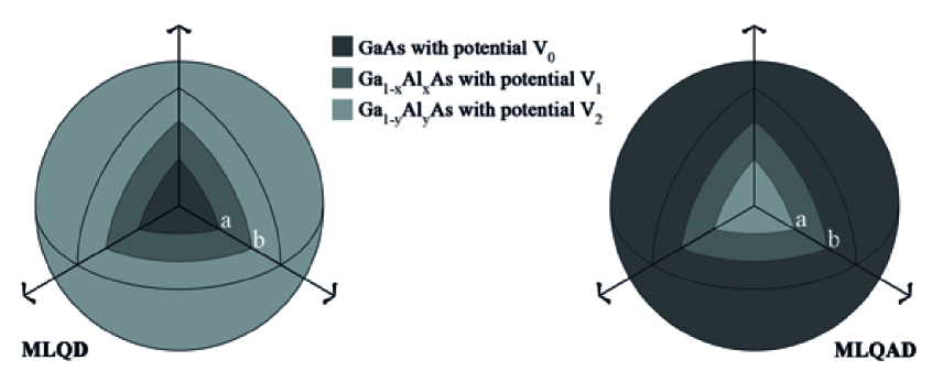
Figure 1: A schematic view of the MLQD and MLQAD structures

Within the framework of the effective mass approximation and in the spherical coordinate system, the Hamiltonian for the MLQD (MLQAD) with hydrogenic impurity in center is given by

$$\hat{H}=-\frac{\hbar^{2}}{2m(r)}\nabla^{2}-\frac{e^{2}}{4\pi\varepsilon r}+V(r)$$ (1)

where $m(r)$ and $\varepsilon$ are the electronic effective mass and dielectric constant in the semiconductor medium. $m(r)$ is represented as follows

$$m(r)=\left\{\begin{array}[]{ll}m_{1}&\hskip 42.67912ptr<a\\ m_{2}&\hskip 42.67912pta\leq r\leq b\\ m_{3}&\hskip 42.67912ptr>b\end{array}\right.$$ (2)

$V(r)$ is the CP and arises due to a mismatch between the electronic affinities of the two regions. The barrier height $V_{1}$ ($V_{2}$) arises in layer Ga_1-xAl_xAs (Ga_1-yAl_yAs) when it binds to the GaAs (Ga_1-xAl_xAs). According to fig. 1, the potential energy $V(r)$ in Eq. 1, for MLQD is

$$V(r)=\left\{\begin{array}[]{ll}V_{0}&\hskip 42.67912ptr<a\\ V_{1}&\hskip 42.67912pta\leq r\leq b\\ V_{2}&\hskip 42.67912ptr>b\end{array}\right.$$ (3)

and for MLQAD is

$$V(r)=\left\{\begin{array}[]{ll}V_{2}&\hskip 42.67912ptr<a\\ V_{1}&\hskip 42.67912pta\leq r\leq b\\ V_{0}&\hskip 42.67912ptr>b\end{array}\right.$$ (4)

the value of $V_{0}$ is always zero (i.e., the GaAs material have no CP) but writing $V_{0}$ helps us to be able to write next equations in the compact form as you will see.

Since the potential is spherically symmetric, we are going to use the spherical coordinates. In the three dimensional spherical coordinate, the Schrödinger eigenvalue equation is $\hat{H}\psi(r,\Omega)=E\psi(r,\Omega)$, where the eigenfunctions are of the separable form $\psi(r,\Omega)=R(r)Y(\Omega)$. For the $r$-dependent (spherically symmetric) potentials, the angular dependence of the wave function, $Y(\Omega)$, is given by the spherical harmonics zet . In particular, the angular part is unaffected by the core and total radius, thus we ignore this part. The radial part is affected by not only the core and total radius but also the dot or antidot CPs, and hence, we consider it in the following subsections.

2.1 MLQAD

Using the method of separation of variables in Schrödinger equation (1), the radial eigenvalue equation in the spherical coordinate in this case can be expressed as

$$\frac{\hbar^{2}}{2m}(\frac{d^{2}}{dr^{2}}+\frac{2}{r}\frac{d}{dr}-\frac{l(l+1)}{r^{2}})R^{(i)}(r)$$ (5)

$$+ (E-V_{i}+\frac{e^{2}}{4\pi\varepsilon r})R^{(i)}(r)=0,$$

where $i=2$, $1$ and $0$ are corresponding to $r<a$, $a\leq r\leq b$ and $r>b$ respectively. Just as we can see in naimi , we can solve this equation as follows. Using the following definitions

$$\alpha^{2}_{i}=\frac{-8m(E-V_{i})}{\hbar^{2}},\ \ \ \ \xi_{i}=\alpha_{i}r,\ \ \ \lambda_{i}=\frac{2me^{2}}{4\pi\varepsilon\hbar^{2}\alpha_{i}^{2}}.$$ (6)

and the change of variable as $W(\xi_{i})=\xi_{i}R^{(i)}(r)$, then the above Schrödinger equation can be rewritten as following Whittaker equation

$$\frac{d^{2}W(\xi_{i})}{d\xi_{i}^{2}}+\left(\frac{-1}{4}+\frac{\lambda_{i}}{\xi_{i}}+\frac{\frac{1}{4}-(l+\frac{1}{2})^{2}}{\xi^{2}_{i}}\right)W(\xi_{i})=0,$$ (7)

The general solution to this equation is the Whittaker functions abra

$$W(\xi_{i})=C_{1i}M_{\lambda_{i},l+\frac{1}{2}}(\xi_{i})+C_{2i}U_{\lambda_{i},l+\frac{1}{2}}(\xi_{i}),$$ (8)

where $C_{1i}$ and $C_{2i}$ are constants to be determined by continuity, asymptotic and normalization conditions. The asymptotic behavior indicates that the wave function must be finite and zero in origin neighborhood and far away from origin, respectively. These conditions lead to $C_{22}=C_{10}=0$ (since $U_{\lambda_{i},l+\frac{1}{2}}(\xi_{i})$ and $M_{\lambda_{i},l+\frac{1}{2}}(\xi_{i}$) diverge at the origin and infinity, respectively). Now one can write the wave functions in three regions as

$$R^{(2)}=C_{12}\frac{M_{\lambda_{2},l+\frac{1}{2}}(\xi_{2})}{\xi_{2}},\ \ \ \hskip 56.9055ptr<a,$$ (9)

$$R^{(1)}=\frac{C_{11}M_{\lambda_{1},l+\frac{1}{2}}(\xi_{1})+C_{21}U_{\lambda_{1},l+\frac{1}{2}}(\xi_{1})}{\xi_{1}},\ \ \ \ a\leq r\leq b,$$

(10)

$$R^{(0)}=C_{20}\frac{U_{\lambda_{0},l+\frac{1}{2}}(\xi_{0})}{\xi_{0}},\ \ \ \hskip 56.9055ptr>b.$$ (11)

2.2 MLQD

The radial eigenvalue equation (5) is also valid for MLQD but according to different definitions of $V(r)$ for MLQD (see Eq. (3) and (4)), in this case we should use $i=0$, $1$ and $2$ for $r<a$, $a\leq r\leq b$ and $r>b$ regions, respectively. In the case of MLQD, the Eq. (5) has been solved in detail by Hsieh et al. in cheng , so we do not directly solve this equation and we shortly review their results for three different regions as follows

(i=0)

Inside the core of system ($r<a$) with $V_{0}=0$, the positive energy bound states are possible for an electron that is confined inside the core dot; therefore, solutions of the Schrödinger equation can be studied in three energy states cheng

• $E<0$

  $$R^{(0)}({\xi_{0A}})$$ (12)

  $$= C_{0A}e^{-\xi_{0A}/2}\xi_{0A}^{l}M(l+1-\lambda_{0},2l+2,\xi_{0A})$$

  where $C_{0A}$ is the normalization constant and $M$ is the first kind of confluent hypergeometric function. The used parameters in the above solution are

  $$\xi_{0A}=\sqrt{\frac{-8mE}{\hbar^{2}}}r,\ \ \ \lambda_{0}=\frac{e^{2}}{4\pi\varepsilon\hbar}\sqrt{\frac{m}{-2E}}.$$ (13)

• $E>0$

  $$R^{(0)}(\xi_{0B})=C_{0B}\sum^{\infty}_{k=l+1}A^{l}_{k}(\beta_{0})\xi^{k-1}_{0B}.$$ (14)

  Similar to the case of $E<0$, $C_{0B}$ is the normalization constant. The recurrence relation $A^{l}_{k}$ function and the other parameters are defined as

  $$A^{l}_{l+1}(\beta_{0})=1,$$ (15)

  $$A^{l}_{l+2}(\beta_{0})=\frac{\beta_{0}}{l+1},$$ (16)

  $$A^{l}_{k}(\beta_{0})$$ (17)

  $$= \frac{2\beta_{0}A^{l}_{k-1}(\beta_{0})-A^{l}_{k-2}(\beta_{0})}{(k+l)(k-l-1)}\hskip 19.91684ptk>l+2,$$

  $$\xi_{0B}=\sqrt{\frac{8mE}{\hbar^{2}}}r,\ \ \ \ \beta_{0}=\frac{e^{2}}{4\pi\varepsilon\hbar}\sqrt{\frac{m}{2E}}.$$ (18)

• $E=0$

  $$R^{(0)}(\alpha_{0C}r)=C_{0C}r^{(-1/2)}J_{2l+1}(\alpha_{0C}\sqrt{r}),$$ (19)

  $C_{0C}$ is the normalization constant and $J_{2l+1}$ is the Bessel function. $\alpha_{0C}$ is defined as

  $$\alpha_{0C}=\sqrt{\frac{8me^{2}}{4\pi\varepsilon\hbar^{2}}}.$$ (20)

(i=1)

For $a\leq r\leq b$
Using the convenient parameters (6), the Schrödinger equation in this region can be expressed in term of Whittaker equation as Eq. (7) which has a result just as the result of (10). In other words, the middle layer in both MLQD and MLQAD behaves in a similar way.

(i=2)

For $r>b$
In this case, similar to the above case, the Schrödinger equation can be expressed in terms of Whittaker equation as Eq. (7) but by using the asymptotic condition in infinity (the M function diverges at infinity), the solution of equation can be written as

$$R^{(2)}(\xi_{2})=C_{2}e^{-\xi_{2}/2}\xi^{l}_{2}U(l+1-\lambda_{2},2l+2,\xi_{2})$$ (21)

where the parameters $\xi_{2}$ and $\lambda_{2}$ are defined as (6). For reading with full detail refer to cheng .

2.3 Linear and nonlinear absorption coefficients

By using the density matrix formalism, the optical properties for a spherical nano-system can be calculated. For this purpose the system under study can be excited by an external electromagnetic field of frequency $\omega$,

$$E(t)=\tilde{E}e^{i\omega t}+\tilde{E}e^{-i\omega t}$$ (22)

If $E$ is the perpendicular electromagnetic field along the $z$ axis, the Hamiltonian of system in this case is $H_{0}+ezE(t)$ where where $H_{0}$ is the Hamiltonian of system without the electromagnetic field $E(t)$. The linear and third-order nonlinear optical absorption coefficients of a spherical nano-system, within a two-level system (in a special case, from ground state to first allowed excited state), can be expressed as saf ; zha ; kho

$$\alpha^{(1)}(\omega)=\omega\sqrt{\frac{\mu}{\varepsilon_{R}}}\frac{\sigma_{v}\hbar\Gamma_{21}|M_{21}|^{2}}{(E_{21}-\hbar\omega)^{2}+(\hbar\Gamma_{21})^{2}},$$ (23)

$$\alpha^{(3)}(\omega,I)$$ (24)

$$= -\omega\sqrt{\frac{\mu}{\varepsilon_{R}}}(\frac{I}{2\varepsilon_{0}n_{r}c})\frac{4\sigma_{v}\hbar\Gamma_{21}|M_{21}|^{4}}{[(E_{21}-\hbar\omega)^{2}+(\hbar\Gamma_{21})^{2}]^{2}}$$

where, $\mu$, $\sigma_{v}$ and $n_{r}$ are the permeability, carrier density and refractive index of the system respectively. $\hbar\omega$ is the incident photon energy, $\Gamma_{21}=1/T_{21}$, $T_{21}$ is the relaxing time between states 1 and 2, $I$ is the optical intensity of incident wave and $c$ is the speed of light in the free space. The remained quantities are defined as

$$E_{21}=E_{2}-E_{1},$$

$$\varepsilon_{R}=n^{2}_{r}\varepsilon_{0},$$

$$M_{21}=|<\psi_{2}|ez|\psi_{1}>|,$$ (25)

where $M_{21}$ is an element of electric dipole moment matrix that in the spherical coordinate is $|<\psi_{2}|er\cos\theta|\psi_{1}>|$.

Finally, the total absorption coefficient is

$$\alpha(\omega,I)=\alpha^{(1)}(\omega)+\alpha^{(3)}(\omega,I).$$ (26)

3 Results and discussion

In this section, we calculate the linear, nonlinear and total absorption coefficients for different shell thicknesses and CPs for both MLQAD and MLQD. The unchanged parameters used in our calculations are : $\Gamma_{21}=0.2ps$, $\sigma_{v}=3.0\times 10^{22}$, $n_{r}=3.2$, $\varepsilon_{R}=13.18$.
Figs. 2(a) and (b) are related to the linear, nonlinear and total absorption coefficients as a function of incident photon energy for MLQAD and MLQD respectively, when $I=20MW/m^{2}$, $a=2a_{0}$, $b-a=0.5a_{0}$, $V_{1}=2Ry$ and $V_{2}=5Ry$. From Fig. 2, it is clear that the ACs of the MLQD and MLQAD have different performances with respect to incident photon energy in the same condition. In the case of comparing the total AC curves, Fig. 2 shows that the MLQD has an approximately symmetric curve but MLQAD has a curve that abruptly increases then asymptotically goes to zero. In the case of the nonlinear AC curves, it is obvious that for this selected intensity value, the MLQD has no significant nonlinear AC but the MLQAD shows a significant nonlinear AC.

 

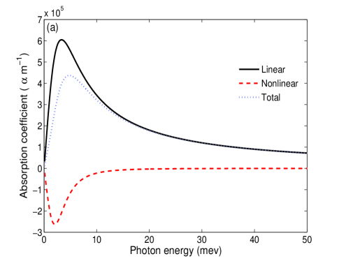
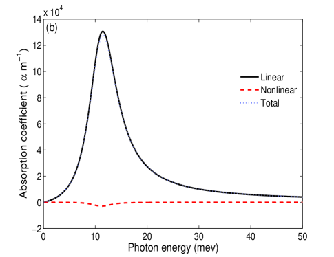
Figure 2: The linear, the nonlinear and the total ACs as a function of incident photon energy in the same condition $\{I=20MW/m^{2}$, $b-a=0.5a_{0}$, $V_{1}=2Ry$ and $V_{2}=5Ry\}$ for (a) MLQAD (b) MLQD.

Figs. 3 (a) and (b) show the linear, nonlinear and total absorption coefficients as a function of the photon energy for MLQAD and MLQD respectively. The solid curves represent linear ACs where as in (22) are independent of intensity, the dashed (dotted) curves display the nonlinear (total) ACs curves. It is observed that,as the optical intensity increases, the total AC decreases for both MLQD and MLQAD. This is because the nonlinear absorption (which is negative) enhances with an increase in intensity. In Fig. 3(a) that shows the behavior of MLQAD, for total ACs curves, from up, the intensity value goes from $I=5MW/m^{2}$ to $30MW/m^{2}$ at fixed incremental steps of $5MW/m^{2}$. If this range of intensity is used for the MLQD, one can see that the MLQD has no significant changes in the nonlinear AC and therefore in the total AC (Fig. 2(b) is the special case of $I=20MW/m^{2}$ that the MLQD has no significant nonlinear AC) we used the range $100\leq I\leq 600$ with a the fixed incremental steps of $100MW/m^{2}$ as the Fig. 3(b) shows it. In this case, at sufficiently high intensity, the nonlinear term causes a collapse at the center of the total AC peak that leads to the splitting of the AC peak into two peaks.

 

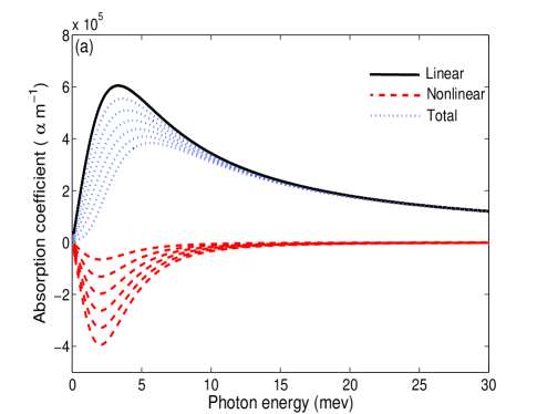
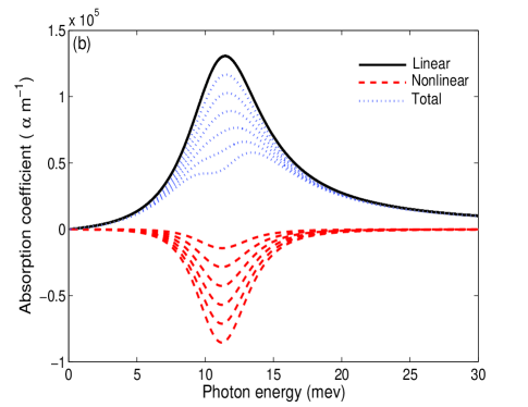
Figure 3: The linear, the nonlinear and the total ACs as a function of incident photon energy with the fixed parameters $\{a=2a_{0},b-a=2.5a_{0},V_{1}=2Ry$ and $V_{2}=5Ry\}$ and six different intensities for (a) MLQAD that from up, the intensity value goes from $I=5MW/m^{2}$ to $30MW/m^{2}$ at fixed increments of $5MW/m^{2}$ (b) MLQD that the range of intensity is $100\leq I\leq 600$ with the fixed incremental steps of $100MW/m^{2}$.

 

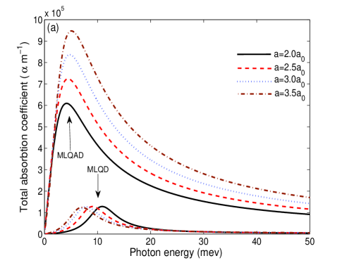
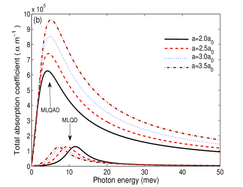
Figure 4: The total AC of MLQD and MLQAD as a function of incident photon energy with the fixed shell thickness $b-a=1a_{0}$ and four different core radii for (a) $V_{1}=2Ry$ and $V_{2}=5Ry$ (b) $V_{1}=2Ry$ and $V_{2}=\infty Ry$.

In Fig. 4(a), the total AC of both the MLQAD and MLQD are plotted when the shell thickness and CPs are fixed as $b-a=1a_{0}$ and ($V_{1}=2Ry,V_{2}=5Ry$) whiles a core radius has a four different values as $a=2,2.5,3,3.5a_{0}$. The graph shows that in lower incident photon energies, the total AC is mainly happened in MLQAD case and by increasing the amount of core radius, the total AC peak heights becomes larger and slightly shift toward larger incident photon energies. In the case of the MQAD, by increasing the core radius value, the peak heights corresponding to MLQD has no significant changes, but move toward the smaller incident photon energies. Figs. 4(a) and (b) are plotted in the same condition, however their difference is in their $V_{2}$ values, where $V_{2}=5Ry$ in Fig. 4(a) and $V_{2}=\infty$ in Fig. 4(b). Regarding these two figures, no considerable changes are observed.

The total AC curves of the MLQAD and MLQD for four different shell thickness $b-a=1,0.5,0.25,0.02a_{0}$, as the function of photon energy are plotted in Figs. 5. In Fig. 5(a) the selected CPs and core radius are $V_{1}=2Ry,V_{2}=5Ry$ and $a=2.0a_{0}$ that by increasing the shell thickness, the peak of total AC curves corresponding to MLQAD moves to larger total AC values without considerable changes in incident photon energy, however the curves related to MLQD shift to smaller energy regions without considerable changes in peak heights. Fig. 5(b) shows the behaviour of the MLQAD and MLQD with the same conditions as Fig. 5(a) with new CPs $(V_{1}=2Ry,V_{2}=\infty Ry)$. By comparing the mutual corresponding curves for example dash-dot curves in Figs. 5 (a) and (b), it is observed that in the biggest shell thickness one can ignore the differences between the total AC curves but in the smaller shell thicknesses, the curves are more affected by changes in CPs.

Generally, from Figs. 4 and  5 it is found that under the same conditions, the total AC in MLQAD is greater than MLQD and also by increasing the shell thickness and core radius, the peak height of MLQAD is more sensitive and becomes significant larger, so we conclude that the utilization of MLQAD structures is more useful.

 

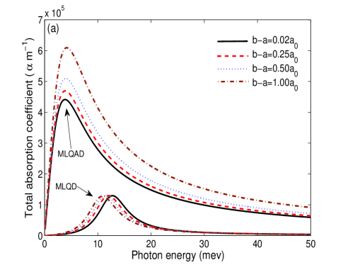
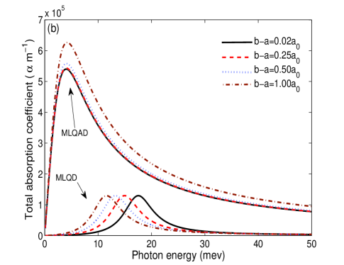
Figure 5: The total AC of MLQD and MLQAD as a function of incident photon energy with $a=2a_{0}$ and four different shell thicknesses for (a) $V_{1}=2Ry$ and $V_{2}=5Ry$ (b) $V_{1}=2Ry$ and $V_{2}=\infty Ry$.

4 Conclusion

By studying the case of multi-layered spherical nano-systems with a hydrogenic impurity, the linear, third-order nonlinear and total optical ACs have been calculated. As our results indicates, in the case of the MLQAD the absorption curves abruptly increase then asymptotically go to zero but in the case of MLQD the absorption curves have symmetrical shapes. Furthermore, the range of variation of intensity that leads to significant changes in total AC curves is different for MLQAD and MLQD. It is observed that for the fixed shell thickness, by increasing the amount of core radius, the total AC peak heights become larger and slightly shift toward larger incident photon energies for MLQAD but the peak heights corresponding to MLQD have no significant changes but move toward the smaller incident photon energies. Also, in this case the change in CPs leads to no considerable changes in total AC curves. Moreover, for a fixed core radius, by increasing the shell thickness, the peak of total AC curves corresponding to MLQAD, moves to larger values without considerable changes in the incident photon energy but the curves related to MLQD shift to smaller energy regions without considerable changes in peak heights. Finally, it is found that in the latter case, by decreasing the shell thicknesses, the total AC curves are considerably affected by CPs values.

- (1) Davatolhagh, S., Jafari, A. R., and Vahdani, M. R. K.: Superlattices and Microstruchure, 51 62 (2012)
- (2) Holovatsky, V. A., Makhanets, O. M., and Voitsekhivska, O. M.: Physica E 41 1522 (2009)
- (3) Varshni, Y. P.: Phys. Lett. A 252 248 (1999)
- (4) Sadeghi, E.: Physica E 41 1319 (2009)
- (5) Vaseghi. B., Rezaei, G., Azizi, V., and Taghizadeh, F.: Physica E 43 1080 (2011)
- (6) Hsieh, C. Y., and Chuu, D. S. J.: Phys. Condens. Matter 12 5641 (2000)
- (7) Naimi, Y., and Jafari, A. R.: J. comput Electron 11 414 (2012)
- (8) Atanasov, R., Bassani, F., and Agranovich, V. M.: Phys. Rev. B 50 7809 (1994)
- (9) Tsang, L., Ahn, D., and Chuang, S. L.: App. Phys. Lett. A 362 37 (2007)
- (10) Karimi, M. J., and Rezaei, G.: Physica B 406 4423 (2011)
- (11) Yang, W., Song, X., Li. R., and Xu, Z.: Phys. Rev. A 78 023836 (2008)
- (12) Xie, W., and Liang, S.: Physica B 406 4657 (2011)
- (13) Bockelman, U., and Bastard, G.: Phys. Rev. B 45 1688 (1992)
- (14) Troccoli, M., Belyanin, A., Capasso, F., Kubukcu, E., Sinco, D. J., and Cho, A. Y.: Nature 433 845 (2005)
- (15) Jiang, X., Li, S. S., and Tidrow, M. Z.: Physica E 5 27 (1999)
- (16) Liu, C., and Xu, B.: Phys. Lett. A 372 888 (2008)
- (17) Lent, C. S., Tougaw, P. D., Porod, W., and Bernstein, G. H.: Nanotechnology 4 49 (1993)
- (18) Unlu, S., Karabulut, I., and Safak, H.: Physica E 33 319 (2006)
- (19) Wei, R., and Xie, W.: Current Applied Physics 10 757 (2010)
- (20) Li, X. C., Wang, AM., Wang, Z. L., and Yang, Y.: Superlattice and Microstructures 51 580 (2012)
- (21) Zhang, C., Wang, Z., Gu, M., Liu, Y., and Guo, K.: Physica B 405 4366 (2010)
- (22) Liang, S., Xie, W., Sarkisyan, H. A., Meliksetyan, A.V., and Shen, H.: Superlattice and Microstructures 51 868 (2012)
- (23) Karabulut, I., and Baskoutas, S. J.: App. Phys. 103 073512 (2008)
- (24) Cakir, B., Yakar, Y., and Ozmen, A.: Journal of Luminescence 132 2659 (2012)
- (25) Ozmen, A., Yakar, Y., Cakir, B., and Atav, U.: Optic Communications 282 3999 (2009)
- (26) Kordad, R.: Indian. J. Phis 86 513 (2012)
- (27) Efros, A. Al., and Efros A.: Sov. Phys. Semicond. 16 772 (1982).
- (28) Zettili, N.: Quantum Mechanic, Concept and Application, pp. 287-289. Wiley, New York (2001)
- (29) Abramowitz, A., Stegun, I.: Handbook of Mathematical Function with Formulas, Graphs and Mathematical Tables, pp. 505-509. US GPO, Washington (1994)
- (30) Adachi, S.: J. Appl. Phys. 58, R1 (1985)