Semiclassical Approach to the Physics of Smooth Superlattice Potentials in Graphene

Abstract

Due to the chiral nature of the Dirac equation, governing the dynamics of electrons in graphene, overlying of an electrical superlattice (SL) can open new Dirac points on the Fermi-surface of the energy spectrum. These lead to novel low-excitation physical phenomena. A typical example for such a system is neutral graphene with a symmetrical unidirectional SL. We show here that in smooth SLs, a semiclassical approximation provides a good mathematical description for particles. Due to the one-dimensional nature of the unidirectional potential, a wavefunction description leads to a generalized Bohr-Sommerfeld quantization condition for the energy eigenvalues. In order to pave the way for the application of semiclassical methods to two dimensional SLs in general, we compare these energy eigenvalues with those obtained from numerical calculations, and with the results from a semiclassical Gutzwiller trace formula via the beam-splitting technique. Finally, we calculate ballistic conductivities in general point-symmetric unidirectional SLs with one electron and one hole region in the fundamental cell showing only Klein scattering of the semiclassical wavefunctions.

I Introduction

Suspended graphene samples exhibit high electron mobilities, where ballistic transport is seen for samples up to the micron length Morozov1 ; Du1 ; Bolotin1 . Within the tight-binding approximation, the graphene system shows two inequivalent momentum energy knots in the Brillouin zone at low energies, located at momenta ${\bf K}$ and ${\bf K}^{\prime}$. An effective low-energy description around these points is given by a massless Dirac equation. Electrons close to these points are related to each other by time-inversion symmetry Castro1 . The effective quasi-relativistic Hamiltonian is then given by

$$H=\hbar v_{F}\left(\frac{1}{i}\sigma_{x}\partial_{x}+\frac{1}{i}\sigma_{y}\partial_{y}\right)+V({\bf r})$$ (1)

for electrons near the ${\bf K}$ point. Here $v_{F}$ is the electron velocity in graphene and $V({\bf r})$ denotes an external potential.

In the energy spectrum of the associated Schrödinger equation, minigaps are opened by the application of an overlying superlattice potential. New bands arise and two of them may touch each other at certain momenta, showing up in new Dirac points. These points are classified by their local similarity of the energy spectrum with the spectrum of the massless Dirac equation. Besides this, they show locally a chiral behavior in the pseudospin expectation value ($\langle\sigma_{x}\rangle,\langle\sigma_{y}\rangle$) as a function of the Bloch momentum Brey1 .

This was first claimed theoretically by Park et al. Park1 ; Park5 , and in fact new Dirac points were found experimentally quite recently for graphene on a hexagonal boron nitride substrate Yankowitz1 . New Dirac points are found at momenta $G_{m}/2$, where $G_{m}$ is a reciprocal lattice wavevector of the SL. Their energies are $E_{D}=\pm\hbar v_{F}|G_{m}|/2$ Park1 . Due to their nonzero energies, these new Dirac points cannot be observed experimentally in low-energy excitation experiments on neutral graphene.

Later on, additional new Dirac points were found in theoretical analyses, all located at zero energy. The calculations were done for graphene with a superimposed unidirectional electrical superlattice potential Brey1 ; Park2 . Actually, these new Dirac points had already appeared earlier in the literature within the framework of an unidirectional SL on a nanotube Talyanskii1 . For the most simple representation of a unidirectional SL step-potential $V(x)=V\chi(x)$, where $\chi(x)={\rm sg}[\sin(2\pi x/d)]$, and ${\rm sg}[x]$ denotes the sign of $x$, the lowest energy band is shown in Fig. 1. The quantity $d$ denotes the wavelength of the SL. The curves were obtained from a precise numerical diagonalization. The full energy spectrum of the lowest band energy shows a mirror symmetry at the $p_{x}$ and $p_{y}$ axes.

The energy spectrum close to the Dirac points is given by Barbier1 ; Dietel2

$$\epsilon_{s}=\!\!sv_{F}\tilde{\alpha}^{2}_{0}\sqrt{p^{2}_{x}+|\hat{\Gamma}|^{2}p_{y}^{2}}\,,\\$$ (2)

with $\alpha_{0}={\color[rgb]{0,0,0}([V/v_{F}]^{2}}-p_{y}^{2})^{1/2}d/2\hbar$, $\hat{\Gamma}=\sin[\alpha_{0}]e^{i\alpha_{0}}/\alpha_{0}$, $\tilde{\alpha}_{0}=\alpha_{0}/\tilde{V}$ where $\tilde{V}=Vd/2\hbar v_{F}$. The Bloch momenta in $x$-direction lie in the Brillouin zone $-\pi/d\leq p_{x}/\hbar\leq\pi/d$. The parameter $s$ distinguishes the conduction band ($s=1$) from the valence band ($s=-1$). From this we deduce that the Fermi-velocity ${\bf v}=\hbar\partial\epsilon_{s}/\partial{\bf p}$ is in general anisotropic at the central valley Dirac point Park3 . The new Dirac points are located at momenta $p_{x}=0$ and $p_{y}d/2\hbar=\pm(\tilde{V}^{2}-(\pi n)^{2})^{1/2}$ with integer $n\in\mathbb{N}$, where $p_{y}$ takes real values. Furthermore, for momenta beyond the new Dirac points we obtain $|p_{y}|\gg V/v_{F}$ the energy $\epsilon_{s}\sim sv_{F}|p_{y}|$ Dietel2 .

These new zero-energy Dirac points differ from the above mentioned points of Park et al. Park1 , since they are not located at momenta with certain fractions of the reciprocal lattice. It is well known that these momenta are part of the region where SL minibands are formed. The Dirac points are then touching points of two minibands. In the case of the zero-energy Dirac points, due to the unidirectional SLs, the pristine Dirac cones are deformed strongly due to electrical potential such that the electron and valence bands touch.

These new Dirac points are located at zero energy, and for that reason they possess a number of new interesting transport properties Brey1 ; Burset1 ; Barbier2 ; Sun1 ; Park4; Dietel1 ; Dietel2 . By an application of an additional magnetic field, new Quantum-Hall plateaus are found Park2 . In disordered SLs, there may also exist interesting localization phenomena Zhu1 .

Figure 1: Lowest energy band $\epsilon d/2\hbar v_{F}$ for the Bloch momentum $p_{x}=0$ and several SL potentials $V(x)=V\chi(x)$ as function of the dimensionless transversal momentum $p_{y}d/2\hbar$.

A general understanding of the energy spectrum, and especially the location of new Dirac points, for general two dimensional non-unidirectional potentials is still missing. Most interesting is the low-energy sector of the energy spectrum in neutral graphene. By taking into account that the zero-energy Dirac points show up only at large SL potentials, semiclassical methods may be used to determine the lowest energy bands for general smooth SLs. To justify this claim we demand that for unidirectional potentials the semiclassical condition

$$\hbar v_{F}\frac{|(E-V)(V^{\prime})|}{\sqrt{(E-V)^{2}-(v_{F}p_{y})^{2}}^{3}}\ll 1$$ (3)

should be fulfilled, except at a few penetration points where

$$\sqrt{[E-V(x_{p})]^{2}-(v_{F}p_{y})^{2}}=0.$$ (4)

Here $V^{\prime}(x)$ is the derivate of the potential $V$ with respect to $x$. In classical mechanics, these points correspond to turning points. Due to the chiral nature of (1) however this is no longer true. For example at the transverse momentum $p_{y}=0$, the transmission probability at the penetration points is unity. Here the electron transforms from a particle state (electron-like) to a hole state (positron-like) or vice versa. This is the analog of Klein’s paradox Klein1 ; Hansen1 ; Greiner1 in relativistic quantum mechanics. In this context it was shown later by Sauter Sauter1 , that the transmission probability is decreasing for non-zero momenta $p_{y}$, and approaching zero for $v_{F}p^{2}_{y}/\hbar V^{\prime}(x_{p})\gg 1$.

In order to prepare the semiclassical approach for smooth SLs, in Sect. II we shall first discuss the semiclassical wavefunctions of the problem. Then we derive transmission and reflection coefficients for electrons or holes, carrying out Klein’s scattering analysis through classically forbidden regions between two penetration points. We apply our results to the simplest unidirectional SL with one electron and one hole region in the fundamental cell, showing only Klein scattering. Our semiclassic results for the lowest energy bands compare well with those obtained numerically. Furthermore, we address the question whether one can construct SLs within the semiclassical approximation which show the ability to focus electron beams. In order to see in which way a semiclassical approach could work also beyond the unidirectional SL case, in Sect. III we consider the generalization of the Gutzwiller trace formula that includes also the beam splitting phenomenon in the calculation of the semiclassical density of states. When calculated from small-length orbits, the density of states will permit us to reconstruct the lowest energy band. Finally in Sect. IV, we shall calculate semiclassical conductivity formulas for smooth unidirectional SLs and compare our results with existing calculations in the literature. We restrict ourselves thereby to ballistic transport. Sect. V and Sect. VI contain a summary of the results.

II The semiclassical energy spectrum of the lowest-band

In the following we formulate the semiclassical approach to the quasi-relativistic Dirac equation of electrons in a unidirectional SL (1). The energy spectrum will show mirror symmetry with respect to the transversal momentum $p_{y}$ at the $p_{y}=0$ axis. In the first subsection, the semiclassical solution of the eigenvalue problem will be obtained via the Bohr-Sommerfeld quantization condition for non-relativistic electrons. We obtain very good agreement for the energy spectrum of the lowest band with numerical results for the SL-deformed sinus potential. In the second subsection, we consider an interesting counter example where the semiclassical approach fails.

II.1 Generalized Bohr-Sommerfeld formalism

Starting point is the solution for the semiclassical wavefunction for the Hamiltonian (1). This was previously done in the case of the relativistic Dirac-equation in Refs. Rubinow1 ; Keppeler1 . We use the semiclassical Ansatz ${\color[rgb]{0,0,0}{\bf\Psi}_{s}}(x)=\sum_{n}\hbar^{n}{\bf\Psi}_{n}e^{iS(x)/\hbar}$ in which ${\bf\Psi}_{n}$, $S(x)$ are independent of $\hbar$. Up to the order $\hbar^{0}$ we obtain

$${\bf\Psi}_{s}(x)\!=\!\frac{|E-V(x)|}{v_{F}\sqrt{|p_{x}|}}\binom{s\frac{p_{x}-ip_{y}}{\sqrt{p_{x}^{2}+p^{2}_{y}}}}{1}e^{iS(x)/\hbar+i\phi(x)}e^{ip_{y}y/\hbar}$$ (5)

with

$$p_{x}(x) = \pm\sqrt{\frac{(E-V(x))^{2}}{v_{F}^{2}}-p_{y}^{2}}\,,$$ (6)

$$S(x) = \int^{x}_{x_{p}}dx^{\prime}p_{x}(x^{\prime})\,,$$ (7)

$$\phi(x) = -\frac{p_{y}}{2}\int^{x}_{x_{p}}dx^{\prime}\frac{1}{p_{x}(x^{\prime})}\frac{\partial_{x^{\prime}}(E-V(x^{\prime}))}{(E-V(x^{\prime}))}\,.$$ (8)

Here $s={\rm sg}[E-V(x)]$, and $S(x)$ is the classical eikonal action of the particle. For neutral graphene, the states with $s=1$ are particle-like , and those with $s=-1$ are hole-like. The symbols $p_{x}$, $p_{y}$ denote the momenta of the particle or hole in $x$, $y$-direction. Note that for $\phi=0$ and neglecting the vector part $(s(p_{x}-ip_{y})/\sqrt{p_{x}^{2}+p^{2}_{y}},1)^{T}$ in (5), the wave function ${\bf\Psi}_{s}(x)$ is the semiclassical solution of the massless quasi-relativistic Klein-Gordon wave equation. This means that $\phi(x)$ is a phase correction factor due to the chiral nature of the quasi-relativistic Dirac equation (1). This phase factor has, of course, direct consequences on the semiclassical Bohr-Sommerfeld quantization condition Littlejohn1 ; Keppeler1 . Without proof we note that by taking into account also a homogeneous magnetic field this factor exactly cancels the Maslov index Maslov1 of the turning points such that the Landau level energy ladder starts at zero energy Carmier1 .

We consider in this paper the simplest case of small energies $|E|\ll{\rm max}[|V(x)|]$ where the scattering in a smooth SL is mainly based on the so-called Klein tunneling for $p_{y}^{2}\lesssim{\rm max}[|V(x)|]/v_{F}$. We shall discuss the situation in general also for larger $p_{y}$ at the end of Sect. IIA.

We assume in the following that in the scattering process, incident particles are coming from the left side of the tunnel region with a positive velocity and energy $E-V(x)>0$. The energy $E$ is conserved during the scattering processes considered in this paper. The particle then tunnels from the left penetration point $x_{pL}$ (see Eq.(4)) into a classical forbidden region between the penetration points $x_{pL}$ and $x_{pR}$, where $\sqrt{[E-V(x)]^{2}-(v_{F}p_{y})^{2}}$ is imaginary. Beyond the penetration point $x_{pR}$ on the right hand side of the tunnel region, it will reach the classical allowed hole region, where $\sqrt{[E-V(x)]^{2}-(v_{F}p_{y})^{2}}$ is again real but now we have $E-V(x)<0$. In general in a Klein tunnel process a particle (hole) tunnel through a classical forbidden region into a hole (particle) region.

Besides Klein tunneling, there are also conventional tunneling processes, for example a particle (hole) tunneling through the full hole (particle) region at imaginary $\sqrt{[E-V(x)]^{2}-(v_{F}p_{y})^{2}}$, i.e., where the particle (hole) does not change its signature $s$. We note that Klein tunneling is also referred to as interband scattering in the literature whereas conventional scattering is an innerband scattering event. One can find further discussions on the nature of scattering in graphene e.g. in Refs. Katsnelson2, ; Beenakker1, ; Lewkowicz1, .

By comparing (5)–(8) with the definition of the penetration points (4), we identify a singular behavior of the semiclassical wavefunction at these points. This means that there is still the freedom to linearly combine the basis of semiclassical wavefunction solutions in (5) consisting of left- and right-moving particles or holes with some yet undetermined numerical prefactors in every nonsingular potential sector. This freedom has to be fixed by further physical arguments. As in the quasi non-relativistic case, we achieve this by matching the wavefunction (5) to the $x\rightarrow\pm\infty$ asymptotics of the exact solution of (1) for the linear potential $V(x)=P(x-\overline{x}_{p})$ where $P\approx\partial_{\overline{x}_{p}}V(\overline{x}_{p})\equiv V^{\prime}(\overline{x}_{p})$, with $\overline{x}_{p}\equiv(x_{pR}+x_{pL})/2$. In the following we assume that the SL is smooth in the classically forbidden region, meaning that $V^{\prime}(x)=P$ changes little between the left and right penetration points $x_{pL}$ and $x_{pR}$ where $P>0$. In order to solve this linear potential scattering problem we first use the Ansatz ${\bf\Psi}(x)=\hbar v_{F}[\frac{1}{i}\sigma_{x}\partial_{x}+\sigma_{y}p_{y}/\hbar-Px](1,1)^{T}\varphi(x)$. This leads to a Klein-Gordon-like differential equation for the wavefunction $\varphi(x)$ in (1), in rescaled coordinates reading

$$\left[\partial_{x^{\prime}}^{2}+\frac{1}{4}x^{\prime 2}-\left(\frac{i}{2}+\tilde{p}_{y}^{2}\right)\right]\varphi(x^{\prime})=0$$ (9)

where the dimensionless transversal momentum square $\tilde{p}_{y}^{2}$ is given by

$$\tilde{p}^{2}_{y}=\frac{v_{F}p_{y}^{2}}{2\hbar|P|}$$ (10)

and $x^{\prime}\equiv(2P/\hbar v_{F})^{1/2}x$. It can be solved with the help of special functions Abramowitz1 . By comparing the asymptotics of this solution for $x\to\pm\infty$ with the semiclassical wavefunction (5), we obtain the transmission and reflection coefficients (11), (12) of the scattering of an electron incident from the left at the potential $V(x)=P(x-\overline{x}_{p})$. After a lengthy but straightforward calculation, the reflection $\overrightarrow{R}_{\rm eh}$ and transmission $\overrightarrow{T}_{\rm eh}$ coefficients are found as

$${\color[rgb]{0,0,0}\overrightarrow{T}_{\rm eh}} = e^{-i\pi{\rm sg}[p_{y}]/2}e^{-\pi\tilde{p}^{2}_{y}},$$ (11)

$$\overrightarrow{R}_{\rm eh} = e^{i\vartheta(\tilde{p}^{2}_{y})}\sqrt{1-e^{-2\pi\tilde{p}^{2}_{y}}}\,,$$ (12)

with

$$\vartheta(\tilde{p}^{2}_{y})=-\pi/4+{\rm arg}[\Gamma(i\tilde{p}_{y}^{2})]+\tilde{p}_{y}^{2}-\tilde{p}_{y}^{2}\ln(\tilde{p}_{y}^{2})\,.$$ (13)

Here $\Gamma$ is the Gamma function. In the reflection and transmission coefficients the arrow on top of the coefficients denote the direction of scattering, i.e. from left to right or vice versa. The suffixes $eh$ ($he$) denotes the case where on the left (right) hand side of the scattering region the electron is particle-like and on the right (left) hand side hole like.

Note that a similar calculation for smooth graphene np and npn junctions was carried out in Refs. Cheianov1 ; Sonin1 ; Tudorovskiy1 . In Fig. 2, we show in Fig. 2 the functions $|T|\equiv|\overrightarrow{T}_{\rm eh}(\tilde{p}_{y}^{2})|$, $|R|\equiv|\overrightarrow{R}_{\rm eh}(\tilde{p}_{y}^{2})|$ and $3\pi/4+\vartheta(\tilde{p}^{2}_{y})$, where $\vartheta$ is an increasing function of $\tilde{p}_{y}^{2}$ with limiting values $\vartheta(0)=-3\pi/4$ and $\lim_{\tilde{p}_{y}^{2}\to\infty}\vartheta(\tilde{p}_{y}^{2})=-\pi/2$.

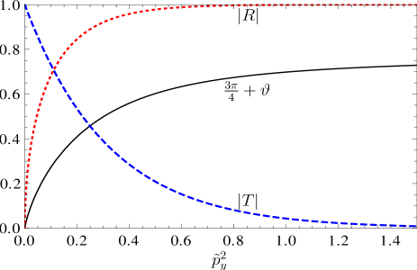
Figure 2: Transmission function $|T|$, reflection function $|R|$, and $3\pi/4+\vartheta$ as a function of $\tilde{p}^{2}_{y}$.

The transmission and reflection coefficient for a hole incident from the right, but again $V^{\prime}(\overline{x}_{p})>0$, can then be determined from (11) and (12), using the invariance of (1) under the transformation ${\bf\Psi}(x)\rightarrow\sigma_{z}{\bf\Psi}^{*}(x)$ for fixed $p_{y}$. This leads to $\overleftarrow{T}_{\rm eh}=\overrightarrow{T}_{\rm eh}$ and $\overleftarrow{R}_{\rm eh}=\overrightarrow{R}^{*}_{\rm eh}$. The transmission and reflection coefficients for a potential with $V^{\prime}(x_{p})\leq 0$ can be read off from the above coefficients by using the substitution $p_{y}\rightarrow-p_{y}$ in the corresponding expressions. This leads to $\overrightarrow{T}_{\rm he}(p_{y})=\overleftarrow{T}_{\rm eh}(-p_{y})$, $\overleftarrow{T}_{\rm he}(p_{y})=\overrightarrow{T}_{\rm eh}(-p_{y})$ and $\overrightarrow{R}_{\rm he}(p_{y})=\overleftarrow{T}_{\rm eh}(-p_{y})$, $\overleftarrow{R}_{\rm he}(p_{y})=\overrightarrow{R}_{\rm eh}(-p_{y})$.

For $\hbar\to 0$ or $p_{y}\to\infty$, finally, we obtain from (11), (12) and (13) that $\overrightarrow{T}_{\rm eh}\to 0$ and $\overrightarrow{R}_{\rm eh}=e^{-i\pi/2}$. Thus in this limit, we obtain the same reflection and transmission coefficient as for the reflection of a non-relativistic particle at a smooth potential barrier Kleinert1 .

The matching procedure used above for the determination of the reflection and transmission coefficients requires that the potential changes little between the penetration points in the classically forbidden region. This has to be fulfilled even in the vicinity of the penetration points. We find from Eq. (3) that $V(x)$ should be almost constant where

$$\quad|x-\overline{x}_{p}|\lesssim\frac{x_{pR}-x_{pL}}{2}+\sqrt{\frac{\hbar v_{F}}{P}}{\rm min}\left[1,\frac{1}{\tilde{p}_{y}^{1/3}}\right]\,.$$ (14)

It is clear that a step-like SL does not fulfil this condition. Note that in the subsequent numerical calculations, we shall use $P{\color[rgb]{0,0,0}\approx}|V(x_{pR})-V(x_{pL})|/(x_{pR}-x_{pL})$ for fixing $\tilde{p}_{y}^{2}$.

Next we calculate the energy spectrum for an unidirectional superlattice potential with two penetration points in the fundamental cell. This configuration is shown in Fig. 3. In order to calculate the eigenvalue spectrum, we have used a transfer matrix method. Note for example that the transfer matrix across the $i$-th penetration point is

$$\underline{M}_{i}=\left(\begin{array}[]{cc}\overrightarrow{T}_{i}-\frac{\overleftarrow{R}_{i}\overrightarrow{R}_{i}}{\overleftarrow{T}_{i}}&\frac{\overleftarrow{R}_{i}}{\overleftarrow{T}_{i}}\\ -\frac{\overrightarrow{R}_{i}}{\overleftarrow{T}_{i}}&\frac{1}{\overleftarrow{T}_{i}}\end{array}\right)\,.$$ (15)

With the definitions

$$S_{i}(x)=(-1)^{i+1}\int_{x_{p_{i1}}}^{x}dx^{\prime}\sqrt{\frac{(E-V(x^{\prime}))^{2}}{v^{2}_{F}}-p_{y}^{2}},$$ (16)

and

$$\underline{N}_{i}(x)=\left(\begin{array}[]{cc}e^{i\frac{S_{i}}{\hbar}(x)}&0\\ 0&e^{-i\frac{S_{i}}{\hbar}(x)}\end{array}\right),$$ (17)

the energy spectrum is given by ${\rm det}[\underline{A}-e^{ip_{x}d/\hbar}\underline{E}]=0$ where $\underline{A}=\underline{M}_{2}\underline{N}_{2}(x_{p22})\underline{M}_{1}\underline{N}_{1}(x_{p12})$, and $\underline{E}$ denotes the unit matrix. The various intersection points $x_{p_{ij}}$ are illustrated for a sinus potential and $E=0$ in Fig. 3. From (8), we obtain that the phase factors $\phi(x)$ in the transfer matrix $\underline{N}_{i}$ are cancelled. By using once more the arguments following (13) we obtain

$$\cos\left(\!\!\frac{S_{1}\!+\!S_{2}}{\hbar}\!\!\right)\!-\!|R_{1}||R_{2}|\cos\!\left(\!\!\frac{S_{1}-S_{2}}{\hbar}\!+\!{\rm arg}[\!\overrightarrow{R}_{1}\!]\!-\!{\rm arg}[\!\overrightarrow{R}_{2}\!]\!\right)$$

$$\quad\quad=|T_{1}||T_{2}|\cos\left(\frac{p_{x}d}{\hbar}\right),$$ (18)

where $S_{i}\equiv S_{i}(x_{pi2})$. In order to obtain a particle-hole symmetry in the spectrum which is the requirement to find new Dirac points for $E=0$, we demand point symmetry of the SL-potential, i.e. $S_{1}=-S_{2}$ for $E=0$. By using the fact that $(1-|R_{1}||R_{2}|)/|T_{1}||T_{2}|>1$ for $|R_{1}|\not=|R_{2}|$, we obtain that Eq. (18) can not be fulfilled for $E=0$ in the case of a potential which has no additional mirror symmetry with respect to the transversal momentum $p_{y}$. This means that semiclassically we do not find any additional Dirac-point except the one for pristine graphene at $p_{x}=p_{y}=0$ for asymmetric potentials where $\overrightarrow{R}_{1}\not=-\overrightarrow{R}_{2}$. Numerically, this is seen using the deformed sinus-potential

$$V(x)=V\sin\left[\frac{2\pi(x-d/2)}{d}\frac{(1+a(x-d/2)^{2})}{1+a(d/2)^{2}}\right],$$ (19)

defined for $0\leq x\leq d$, for calculating the lowest energy band by a numerical diagonalization, and compare the results with the semiclassical ones (18). In Fig. 3 we show these results for various deformed sinus potentials.

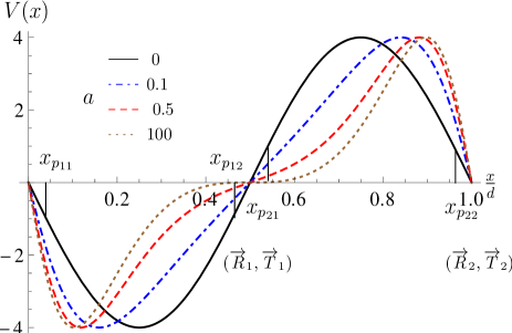
Figure 3: We show the deformed sinus potential (19) for potenial strength $V=4$ and deformation parameters $a=0,0.1,0.5,100$. The various penetration points are shown for the non-deformed sinus potential $a=0$ in the case that $E=0$ and $p_{y}v_{F}/V=1$.

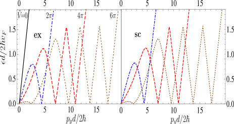
Figure 4: Lowest energy band at $p_{x}=0$ for the non-deformed sinus-potential (19), with $a=0$ and $\tilde{V}=0,2\pi,4\pi,6\pi$. The left panel shows the numerical, the right panel the semiclassical results (18).

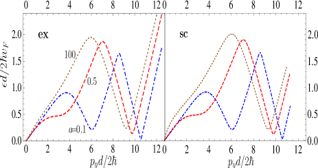
Figure 5: Lowest energy band at $p_{x}=0$ for the deformed sinus-potential (19) with $\tilde{V}=4\pi$ and $a=0.1,0.5,100$. The left panel shows the numerical, the right panel the semiclassical results (18).

In the left panel of Fig. 4, we show the lowest energy band for $p_{x}=0$, using the exact numerical diagonalization method for the various sinus potentials (19), whereas in the right panel the corresponding semiclassical result (18) is shown. The same is shown in Fig. 5 for various deformed sinus-potentials. The plots are characterized by $\tilde{V}(x)\equiv V(x)d/2\hbar v_{F}$ since the energy spectrum (up to a simple rescaling of momentum and energy) as well as the conductivities depend mainly on this dimensionless potential. In both figures we obtain an almost perfect agreement between numerical diagonalization results and semiclassical lowest energy band.

As was already discussed following Eq. (8), the Klein-scattering process dominantes over other scattering processes for small energies $E$ and momenta $p_{y}$ for smooth SLs. Let us elaborate this point further. First we can show using semiclassical methods similar to those applied to the step-like case in Sect. I, that $|\epsilon_{s}|\gtrsim v_{F}|p_{y}|$ at large momenta where $|p_{y}v_{F}|\gg{\rm max}[|V(x)|]$. On the other hand for small momenta where $|p_{y}v_{F}|$ is smaller than the absolute value of possible local minima (maxima) of $V(x)$ in the case of particles (holes), we obtain that mainly Klein scattering processes are active for small energies $|E|\ll|p_{y}v_{F}|$. For momenta $p_{y}$ between these two extrema, also conventional scattering processes are relevant. To avoid them at low energies we must take into account (14), and demand that the SL potential $V(x)$ does not have any local minima (maxima) for particles (holes) and that the local minima and maxima are of similar absolute potential value. Furthermore we must demand that $V^{\prime}(x)\approx{\rm const}$ between the local minima and maxima. The smooth forms of the symmetric two-step potential belong to a class of potentials fulfilling these requirements.

We point out that these requirements are not necessary but sufficient to determine the whole low energy region of the lowest energy band for a given SL potential within the semiclassical method discussed in this paper. The reason that these requirements are not necessary lies in the fact that the type of scattering depends strongly on the energy of the particle or hole. The above requirements hold under the assumption that $|E|\ll|p_{y}v_{F}|$, and this does not have to be fulfilled for certain momentum values $p_{y}$.

II.2 Constructing SLs for focusing electron beams

In the following, we restrict ourselves to unidirectional SLs with a mirror symmetry and an additional point symmetry at the origin similar, to the sinus potential discussed above. As was shown in the last section, this requirement is necessary to find new Dirac points on the $E=0$ axis. For $E=0$ we obtain from (18) $S\equiv S_{1}=-S_{2}$ and $\rm{arg}[\overrightarrow{R}]\equiv\rm{arg}[\overrightarrow{R}_{1}]=-\rm{arg}[\overrightarrow{R}_{2}]$, that the momentum $p_{y}=p_{y}^{n}$ of the new Dirac points is determined by

$$\frac{S}{\hbar}+\rm{arg}[\overrightarrow{R}]=\pi({\color[rgb]{0,0,0}{\it n}}-1)\,,$$ (20)

where $n\in\mathbb{N}$ . The number of new Dirac points is then given by

$$\left[1+\frac{1}{\pi}\left(\frac{S}{\hbar}+\rm{arg}[\overrightarrow{R}]\right)\right]=n_{\rm max}\,,$$ (21)

where we have to set $p_{y}=0$ in $S$ and $\overrightarrow{R}$ entering (21). We have used the abbreviation $[x]$ as the largest integer number smaller than $x$.

As mentioned above and can be deduced from (2) for the unidirectional step-like SL, electrons with a momentum near the central Dirac point are focused strongly in the direction of the SL wavevector, i.e., $v_{x}\gg v_{y}$, especially at potentials where a new Dirac point emerges. It was mentioned in Ref. Park3, that this phenomenon could have technical applications for strong focusing of electron beams in graphene. Of course, true focusing of an electron beam has the additional requirement that $v_{y}=0$ in the vicinity of a specific momentum, and not only exactly for that momentum. Such energy dispersions were in fact found in photonic crystals Kosaka1 ; Rakich1 . Within the semiclassical approximation, by solving (20) in a nontrivial momentum region, we are now able to construct potentials showing exactly such a behavior. For doing this we restrict ourselves to SL potentials in the large $V$-regime of the form $V\sin[2\pi(x-d/2-\delta d)/d]$ for $d/2\leq x_{1}\leq x\leq 3d/4$. Note that due to its symmetry only the discussion of the positive branch of the potential, i.e. for $x$-values where $d/2\leq x\leq 3d/4$, is sufficient. The value $x_{1}$ is given by the condition that (20) is fulfilled for the momentum $p^{1}_{y}=V(x_{1})/v_{F}$ where we only consider in the following $n=1$.

Figure 6: The (black) solid curve (sc) is the semiclassically calculated energy spectrum for the potential $V_{f}$ at $p_{x}=0$ which is shown as the black solid curve in the inset. The other curves (ex) in the main panel are the lowest energy spectra calculated by an exact numerical diagonalization calculation for the potential $V_{f}$ and its variations shown in the inset.

We now determine the potential $V_{f}(x)$ for $d/2\leq x\leq x_{1}$ by solving (20) iteratively. Here we determine $\delta d$ and $V$ such that $V_{f}(d/2)\approx 0$ and further that the momentum value at the first Dirac point $p^{1}_{y}$ is maximal. With these requirement we obtain $2\pi\delta d/d=0.437$ and $\tilde{V}=4.58$.

Within the semiclassical approximation this leads to the fact that the first side-valley Dirac point $p_{y}^{1}$ and the central Dirac point are connected by a flat energy dispersion curve with zero energy. We show in the inset in Fig. 6 as the black solid curve the potential $V_{f}(x)$ obtained in this way. The (red) dotted and the (blue) dashed potential curves are variations of $V_{f}$ being different at $x<x_{1}$-values. The black solid curve denoted with sc in the main panel in Fig. 6 shows then the semiclassically calculated lowest energy spectrum by using (18). Indeed we obtain a flat energy curve around the central Dirac point. The other energy curves shown in the Figure are calculated by using the exact numerical diagonalization method. The various exact diagonalization curves in Fig. 6 correspond to the potential variations shown in the inset. From the (black) solid energy curve can be seen that the flatness of the semiclassical approximation in fact vanishes within the numerical diagonalization calculation. Note that this even holds when going to a high basis number in the exact numerical diagonalization calculation. This shows that the semiclassical approximation fails here for the constructed potential $V_{f}$, at least to the extend of having a flat energy spectrum close to the central Dirac point. The reason for this failure presumably comes from the fact that at the penetration point $x_{p21}=x_{1}$ the condition (14) is no longer fulfilled. Note that $V_{f}$ even gets more shallow when choosing larger $x_{1}p^{1}_{y}$ values where now the energy plateau seen in the semiclassical construction cannot be extended to $p_{y}d=0$.

From Fig. 6 we even obtain from Fig. 6 that the energy curves of the potential variations of $V_{f}$ shown in the inset do not vary much around the central Dirac point. We consider this as a hint that presumably the whole attempt of finding an SL potential with a flat region in the energy spectrum, with one electron and one hole region in the fundamental cell, seems doomed to fail. Note also that we carried out further numerical calculations with variations of the SL potential which turned out to be unsuccessfull as well. It was shown in Ref. Sun1, that such a scheme can be successful when considering more complicated SLs. In that paper it was shown that a SL with one electron and one hole region and an additional small modulation of the potential strengths over many fundamental cells of the SL can lead to energy spectra with a flat behavior around the Dirac points.

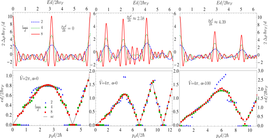
Figure 7: Upper panels show the dimensionless density of states $2\Delta\hbar v_{F}\rho/d$ as a function of the dimensionless energy $Ed/2\hbar v_{F}$ for various maximal orbit lengths $l_{\rm max}$ at $p_{x}=0$. The SL potential is given by the non-deformed sinus potential (19) with $\tilde{V}=2\pi$ and $a=0$. Th density of states is calculated for the central valley where $p_{y}d/2\hbar=0$ (left panel), at transversal momentum value $p_{y}d/2\hbar=2.58$ where we found the maximum of the lowest energy band (middle panel), and at the new side valley Dirac-point momentum $p_{y}d/2\hbar=4.39$ (right panel). Lowers panels show the energy of the lowest maximum value of the density of states $\Delta\rho$ for various orbit lengths $l_{\rm max}$. We compare these values with the semi-classical spectrum calculated by (18) (black curve). We show this for the sinus potential (19) with $\tilde{V}=2\pi$, $a=0$ (left panel); $\tilde{V}=4\pi$, $a=0$ (middle panel) and $\tilde{V}=4\pi$, $a=100$ (right panel).

III Semiclassical density of states

The generalization of the above results to general two-dimensional SLs via a semiclassical wavefunction solution of Eq. (1) is not possible. In the case of non-relativistic quantum mechanical systems this can be carried out only for integrable systems Brack1 . This result is modified in relativistic systems mainly due to the existence of the additional phase factor $\phi(x)$ in (5) Littlejohn1 ; Keppeler1 . One way out of this dilemma is by calculating the density of states semiclassically with a formalism developed by Gutzwiller Gutzwiller1 . The eigenvalue spectrum is then determined from the calculated density of states.

For the unidirectional SL with one electron and one hole region per fundamental cell we obtain for the density of states Bolte1 ; Carmier1 $\rho(E)=\overline{\rho}(E)+\Delta\rho(E)$. Here $\overline{\rho}$ is the average density of states, given by

$$\overline{\rho}(E)\approx\frac{1}{\pi\hbar}\int^{d}_{0}dx{\rm Re}\left[\frac{|E-V(x)|}{v_{F}^{2}\sqrt{\frac{(E-V(x))^{2}}{v_{F}^{2}}-p_{y}^{2}}}\right]\,.$$ (22)

The fluctuating part is given within a semiclassical approximation by

$$\Delta\rho(E)\!=\!\frac{1}{\pi\hbar}{\rm Re}\!\left[\!\sum_{p}\!T_{p}\!\sum_{\nu=1}^{\infty}\![T^{\tau(p)}R^{\sigma(p)}]^{\nu}e^{-i\nu\gamma(p)\frac{p_{x}d}{\hbar}}e^{i\nu\frac{S_{p}}{\hbar}}\right]\!.$$ (23)

The sum $p$ in (23) runs over the primitive periodic orbits of particles $E-V(x)>0$ or holes $E-V(x)<0$, respectively. Particles and holes are transformed into each other at the penetration points. The configuration space of the orbits is given by the fundamental cell of the SL with periodic (circular) boundary conditions. $T_{p}$ is the required time for the particle or hole for passing the primitive orbit. $T^{\tau(p)}$ stands for $T^{\tau(p)}=\overleftarrow{T}_{1}^{\overleftarrow{\tau}_{1}(p)}\overrightarrow{T}_{1}^{\overrightarrow{\tau}_{1}(p)}\overleftarrow{T}_{2}^{\overleftarrow{\tau}_{2}(p)}\overrightarrow{T}_{2}^{\overrightarrow{\tau}_{2}(p)}$. Here $\overrightarrow{\tau}_{i}(p)$ $(\overleftarrow{\tau}_{i}(p))$ is the number of transmissions from left (right) to right (left) through the potential barrier $i$ in the primitive orbit. $R^{\sigma(p)}$ is the corresponding total reflection coefficient. $S_{p}$ is the eikonal of the primitive orbit, i.e. $S_{p}=n_{1}S_{1}+n_{2}S_{2}$ where $n_{1}$ and $n_{2}$ are the number of transitions of the particle regions $E-V(x)>0$ and hole regions $E-V(x)<0$. $\gamma(p)$ is the winding number of the primitive orbit on the circle representing the fundamental cell.

In order to derive Eq. (23), we used the ray splitting generalization of Gutzwiller’s trace formula first discussed in Ref. Couchman1, . There it was shown that a ray splitting boundary in an integrable system can cause additional sign of chaos in the energy spectrum. One of the simplest systems with ray splitting is that of a non-relativistic electron in an infinite one-dimensional square well with a discontinuous step inside the well Dabaghian1 ; Dabaghian2 ; Timberlake1 . This system, and also our system represented by the density of states (23) can be discussed using the formalism of quantum graphs Kottos1 . With the help of the methods used in this reference one can directly show the connection between the density of states (23) and the corresponding energy spectrum represented by equation (18).

By using that the absolute value of the particle velocity is given by $v_{f}\sqrt{(E-V(x))^{2}-p_{y}^{2}v_{F}^{2}}/|E-V(x)|$ one can easily determine $T_{p}$ for every primitive orbit by integrating the inverse velocity over the orbit. It is well known Brack1 that a renumbering of the summands in (23) can lead to divergent subseries. A well-behaved approximation should be achieved by sorting the terms in (23) with respect to their maximal orbit length $l_{\rm max}$. This means that for $l_{\rm max}=2md$ with $m\in\mathbb{N}$ we have to take into account in (23) all orbits with lengths less than or equal to $2md$. In the upper row in Fig. 7 we show $\Delta\rho$ for $l_{\rm max}=2d$ , $4d$ and $8d$ for the sinus potential (19) with $\tilde{V}=2\pi$, $a=0$ and $p_{x}=0$. These panels are calculated for $p_{y}d/\hbar$ values where the lowest energy band (cf. Fig. 4) has its two Dirac points (left and right panel) and further where the band has its local maximum (mid panel). By comparing the curves with the corresponding energy spectrum in Fig. 4 we obtain that the energy values of the lowest energy band correspond to the smallest energy maximum in $\Delta\rho$. This happens even when we take into account only small $l_{\rm max}$ orbit lengths. We note that the higher energy maxima of $\Delta\rho$ in Fig. 7 correspond to higher energy bands. Next we try to reproduce the lowest energy band for various (deformed) sinus potentials and $l_{\rm max}=2d$, $4d$ and $8d$ from the lowest energy maximum in $\Delta\rho$. We compare our result in Fig. 7 with the semiclassically calculated lowest energy band by using (18) ((black) straight curves). We obtain from the figure that the new Dirac points even show up for small $l_{\rm max}$ in form of a plateau at zero energy where its extension is rapidly decreasing for higher $l_{\rm max}$-values. Note that the maximum criterium used here for determing the spectrum from $\Delta\rho$ is different from the common approaches used for determing the full energy spectrum for systems in the field of quantum chaos. There commonly the condition that the integration of the full density of states between two non-degenerate energy levels should give the value one is used. Since we are only interested in the lowest energy level and furthermore the lowest energy band and the first excited energy band are well separated, such an approach is not necessary here.

IV Conductivities

Next, we calculate the conductivities parallel and orthogonal to the SL wavevector by using the semiclassical wavefunction (5) and energy dispersion (18) for SLs with a point symmetry at zero energy for half-filling. We thereby restrict ourselves to the ballistic transport regime. Note that ballistic transport was seen for graphene samples without a SL up to the micron length Morozov1 ; Du1 ; Bolotin1 . Taking into account also the small interlattice spacing of $1.4$ Å  in graphene makes the ballistic transport regime relevant even for large superlattices.

There are various techniques in the literature for calculating ballistic conductivities in graphene. Below, we will use a formalism firstly introduced in Ref. Lewkowicz2, for graphene without a SL. In this approach the linear ballistic transport is calculated as a response to an electric field given by a temporal gauge field of the form ${\bf A}=-c{\bf E}t\Theta(t)$, where ${\bf E}$ is the external electric field.

There are also Kubo-like formalisms in the literature using gauge fields of the spatial form. These have the disadvantage that the calculated conductivities in these formalisms are only well defined up to a numerical prefactor which depends on the order of taking the zero-temperature, zero-frequency, and zero-damping limit Ziegler1 ; Ryu1 . The simplest versions of both of these formalisms above work for non-doped leads. For heavily doped leads a Landauer-like transfer matrix formalism Katsnelson1 ; Tworzydlo1 can be found in the literature for SL-free pristine graphene. Here evanescent modes give the dominant contribution to the conductivity. These modes do not longer fulfill the Bloch condition which makes it complicated to find analytical conductivity results for general smooth SLs. A further complication comes from the fact that in using the semiclassical approach one has to demand that the leads are coupled to the graphene system in a smooth way introducing a new parameter to the system. Finally we note the important fact that the Landauer formalism for heavily doped leads and the temporal gauge formalism for non-doped leads, which we will use below, result in numerical similar conductivity values for pristine graphene.

The lowest band eigenvalue spectrum is given by (18) which was effectively calculated from the eigenvalues of the matrix $\underline{A}$. By using (18) we obtain the following energy dispersion around the Dirac points, i.e. for $|\epsilon_{s}|dI(-1,0)/2v_{F}S\ll 1$,

$$\!\!\!\!\!\!\epsilon_{s}=s\frac{2\hbar v_{F}}{d}\frac{1}{I(-1,0)}\Bigg{[}|T|^{2}\sin^{2}\left(\frac{p_{x}d}{2\hbar}\right)+$$ (24)

$$\!+|R|^{2}\sin^{2}\left(\frac{S+{\rm arg}[\overrightarrow{R}]}{\hbar}\right)+\frac{1}{2}(1-|R|^{2}-|T|^{2})\Bigg{]}^{1/2}$$

where $s=1$ for the conduction band and $s=-1$ for the valence band. Here we use the abbreviation ${\rm arg}[\overrightarrow{R}]\equiv({\rm arg}[\overrightarrow{R}_{1}]-{\rm arg}[\overrightarrow{R}_{2}])/2$ and $|R|\equiv\sqrt{|\overrightarrow{R}_{1}||\overrightarrow{R}_{2}|}$, $|T|\equiv\sqrt{|\overrightarrow{T}_{1}||\overrightarrow{T}_{2}|}$ and denote $\overrightarrow{R}\equiv|R|e^{i{\rm arg}[\overrightarrow{R}]}$ for energies $E=0$. The function $I(n_{1},n_{2})$ is defined by

$$I(n_{1},n_{2})=\frac{2}{d}\int_{x_{pi1}}^{x_{pi2}}\!\!\!dx\,\frac{\sqrt{\left(\frac{V(x)}{v_{F}}\right)^{2}-p_{y}^{2}}^{n_{1}}p^{n_{2}}_{y}}{|V(x)/v_{F}|^{n_{1}+n_{2}}}\,.$$ (25)

In the following, we will use the eigenfunctions of the matrix $\underline{A}$ which was defined following Eq. (18). These are given in the vicinity of the Dirac points, i.e. for $|\epsilon_{s}|dI(-1,0)/2v_{F}S\ll 1$, by

$${\bf EV}\!\!\approx\!i\!\left(\!\!{\sin\!\left[\!\frac{Ed}{\hbar v_{F}}I(-1,0)\!\right]\!\!-\!\!\sin\left[2\frac{S}{\hbar}\!\!+\!\!2{\rm arg}[\overrightarrow{R}]\right]|R|^{2}\!\!+\!\!\frac{p_{x}d}{\hbar}|T|^{2}\atop-e^{i\frac{S}{\hbar}}\left(|R_{1}|e^{i\frac{S}{\hbar}+{\rm arg}[\overrightarrow{R}_{1}]}-|R_{2}|e^{-i\frac{S}{\hbar}+{\rm arg}[\overrightarrow{R}_{2}]}\!\right)\!}\right)$$ (26)

The lowest-band eigenfunctions for electrons in the SL are then given for $0\leq x\leq d$ by

$${\bf u}_{s}(x)\approx\bigg{(}\underline{M}_{1}\underline{N}_{1}(x)\Theta(x-x_{p11})\Theta(x_{p12}-x)$$

$$+\underline{N}_{2}(x)\underline{M}_{1}\underline{N}_{1}(x_{p12})\Theta(x-x_{p21})\Theta(x_{p22}-x)\bigg{)}{\bf EV}/N.$$ (27)

Here $N$ is a normalization constant. Note that we omitted here once more semiclassical phase factors (8) as previously in (18). We show below that they will in fact not contribute to the conductivity within the semiclassical approximation. Furthermore we idealized in (27) the whole wavefunction by setting it to zero in the classical forbidden region. We will also justify this assumption below.

Next we calculate the dc-response in the SL system. This is done in the gauge ${\bf A}=-c{\bf E}t\Theta(t)$. The conductivity in the $i$-th direction in the lowest energy level approximation valid for $t\to\infty$ is then given by Lewkowicz2 ; Dietel2

$$\tilde{\sigma}_{ii}\!=\!\frac{-4ev_{F}}{(2\pi)^{2}}\int_{\rm BZ}\!\!\!\frac{d^{2}p}{\hbar^{2}}\mbox{Re}[e^{-\frac{i}{\hbar}\Delta\epsilon t}\langle{\bf u}_{-1}|\sigma_{i}|{\bf u}_{+1}\rangle\xi_{+}(t)],$$ (28)

with

$$\xi_{+}(t)=-i\frac{ev_{F}}{\hbar}\!\!\int_{t^{\prime}=0}^{t}\!\!\!\!\!dt^{\prime}\!\!\int_{t^{\prime\prime}=-\infty}^{t^{\prime}}\!\!\!\!\!\!\!dt^{\prime\prime}{\cal T}(t^{\prime\prime}),$$ (29)

and the transition matrix element ${\cal T}=e^{\frac{i}{\hbar}\Delta\epsilon t}\langle{\bf u}_{1}|\sigma_{i}|{\bf u}_{-1}\rangle$. The value $\Delta\epsilon$ is given by the energy gap $\Delta\epsilon=\epsilon_{1}-\epsilon_{-1}$ for an electron with momentum $p_{y}$. The integral in (28) is carried out over the full Brillouin zone.

In the following we separately calculate the contribution of every energy valley to the momentum integral in (28), i.e.,

$$\tilde{\sigma}_{ii}=\sum_{n=0}\tilde{\sigma}^{n}_{ii}(2-\delta_{n,0}).$$ (30)

For large times one can restrict the $p_{y}$-integrals of Eq. (28) to the vicinity of the valley center $p_{y}^{n}$ in ${\cal T}$ where $p_{y}^{n}$ is determined by (20) for $n>0$ and $p^{0}_{y}=0$ for the central valley. The factor two in (30) takes into account the mirror symmetry of the energy spectrum with respect to $p_{y}$, such that we may consider only $p^{n}_{y}\geq 0$ in (30).

For calculating the conductivity $\tilde{\sigma}^{n}_{ii}$, we first have to determine the matrix element $\langle{\bf u}_{1}|\sigma_{i}|{\bf u}_{-1}\rangle$. We apply the semiclassical approximation by assuming $\hbar$ being small enough to neglect integrals of the form $\int dxe^{i2\int^{x}dx^{\prime}S_{i}(x^{\prime})/\hbar}$ in comparison to the integrals $\int dxe^{i0\int^{x}dx^{\prime}S_{i}(x^{\prime})/\hbar}$. On similar grounds we may also neglect the matrix contributions in the classical forbidden regions. From this argument it becomes evident that the semiclassical phases $\phi(x)$ (8) will not contribute to $\langle{\bf u}_{1}|\sigma_{i}|{\bf u}_{-1}\rangle$ since the integrand in (8) is inverse proportional to $1/p_{x}(x^{\prime})$.

By using (27)–(29) we obtain the following conductivities

$$\tilde{\sigma}^{n}_{ii}=\frac{1}{2}\frac{e^{2}}{h}\frac{O_{i}}{|v_{x}v_{y}|/v_{F}^{2}}$$ (31)

with $v_{x}$ and $v_{y}$ being the electron velocities at the Dirac point. By using (24) we obtain

$$|v_{x}|=|T|\frac{v_{F}}{I(-1,0)}\,,$$ (32)

$$|v_{y}|=\frac{2v_{F}\hbar}{I(-1,0)d}$$ (33)

$$\times\partial_{p_{y}}\sqrt{|R|^{2}\sin^{2}\left(\frac{S}{\hbar}+{\rm arg}[\overrightarrow{R}]\right){\color[rgb]{0,0,0}+\frac{1}{2}(1-|R|^{2}-|T|^{2})}}\,.$$

The absolute square of the transition matrix elements are given by

$$O_{x}=\int_{0}^{2\pi}d\vartheta\frac{(N^{d}_{x}F^{1}_{-})^{2}}{|N^{d}F^{2}_{+}+N^{nd}F^{3}_{+}||N^{d}F^{2}_{-}+N^{nd}F^{3}_{-}|},$$

$$O_{y}=\int_{0}^{2\pi}d\vartheta\frac{(N^{d}_{y}F^{1}_{+}+N^{nd}_{y}F^{4})^{2}}{|N^{d}F^{2}_{+}+N^{nd}F^{3}_{+}||N^{d}F^{2}_{-}+N^{nd}F^{3}_{-}|}$$ (34)

with

$$N^{d}=\frac{2}{T^{2}}\bigg{\{}\left(\frac{5}{2}+2|R|^{2}\right)I(-1,0)$$

$$+{\rm Re}[\overrightarrow{R}][I(-1,2)-I(-1,0)]+2{\rm Im}[\overrightarrow{R}]I(0,1)\bigg{\}}\,,$$

$$N^{nd}=\frac{4}{|T|^{2}}|R|I(-1,0)\,,$$

$$N^{d}_{x}=4I(0,0)\,,$$

$$N^{d}_{y}=\frac{4}{|T|^{2}}\bigg{\{}{\rm Re}[\overrightarrow{R}][I(-1,1)+{\rm Im}[\overrightarrow{R}]I(0,0)\bigg{\}}\,,$$

$$N^{nd}_{y}=\frac{4}{|T|^{2}}|R|I(-1,1),$$ (35)

and

$$F^{1}_{\pm}\!=\!H_{+}(\vartheta)H_{-}(\vartheta)\!\pm\!\cos^{2}(\vartheta)\,,\,F^{2}_{\pm}\!=\!H^{2}_{\pm}(\vartheta)\!+\!\cos^{2}(\vartheta),$$

$$F^{3}_{\pm}\!=\!2\cos(\vartheta)H_{\pm}(\vartheta)\,,\,F^{4}\!=\!-2\cos(\vartheta)(H_{\pm}(\vartheta)\mp 1),$$ (36)

where

$$H_{\pm}(\vartheta)=\pm 1-|R|\cos(\vartheta)+|T|\sin(\vartheta).$$ (37)

In the following, we further specify the parameters in (31). For the side-valleys $n>0$, the value $p_{y}$ in the expressions (31)-(36) is given by the side-valley Dirac point momentum determined by (20). In this case we obtain for $v_{y}$ (32)

$$|v_{y}|=\frac{2v_{F}}{I(-1,0)}\left[-\frac{1}{2}I(-1,1)+\frac{\hbar}{d}\partial_{p_{y}}{\rm arg}[\overrightarrow{R}]\right]|R|,$$ (38)

with

$$\frac{\hbar}{d}\partial_{p_{y}}{\rm arg}[\overrightarrow{R}]=\frac{1}{4}[{\rm Re}[\Psi(i\tilde{p}_{y}^{2})]-\log(\tilde{p}_{y}^{2})]\bigg{[}\left(\frac{x_{p21}-x_{p12}}{d}\right)$$

$$+\frac{p_{y}v_{F}}{d}\left(\frac{1}{V^{\prime}(x_{p21})}+\frac{1}{V^{\prime}(x_{p12})}\right)\bigg{]},$$ (39)

where $\Psi$ is the digamma function.

For the central valley $n=0$ we have

$$\frac{\hbar}{d}\partial_{p_{y}}|R_{i}|=\sqrt{\frac{\pi\hbar v_{F}}{d^{2}V^{\prime}(x_{pi})}}\,.$$ (40)

Here $x_{pi}$ is the $i$-th intersection point of the SL potential and the x-axis, i.e. $x_{p1}=d/2$ and $x_{p2}=0$. The $p_{y}$ momentum value in the expressions (31)-(39) is then given by $p_{y}=0$. The electron velocity in $y$-direction is for $n=0$ given by

$$\!\!\!\!|v_{y}|\!=\!\frac{2\hbar v_{F}}{dI(-1,0)}\times\Bigg{[}\sin^{2}\left(\frac{S}{\hbar}-\frac{3\pi}{4}\right)(\partial_{p_{y}}|R_{1}|)(\partial_{p_{y}}|R_{2}|)$$

$$~{}~{}~{}~{}~{}~{}~{}~{}~{}~{}~{}~{}~{}~{}~{}\quad\quad\quad+{\color[rgb]{0,0,0}\frac{1}{4}\left(\partial_{p_{y}}|R_{1}|-\partial_{p_{y}}|R_{2}|\right)^{2}\Bigg{]}^{1/2}\!\!.}$$ (41)

The only non-zero values in (35) for $p_{y}=0$ are given by $N^{d}=5$ and $N_{x}^{d}=4$. This leads to $O_{y}=0$ and $O_{x}=16\pi/25$.

For a step-like SL potential $V(x)=V\chi(x)$, the dc-conductivities are given by Burset1 ; Dietel2

$$\tilde{\sigma}^{n}_{xx}=\frac{e^{2}}{h}\,\frac{\pi}{2}\tilde{\alpha}^{2}_{0}\frac{1}{|\Gamma_{n}|}\quad,\quad\tilde{\sigma}^{n}_{yy}=\frac{e^{2}}{h}\frac{\pi}{2}\frac{1}{\tilde{\alpha}^{2}_{0}}|\Gamma_{n}|\,.$$ (42)

with $\tilde{\alpha}_{0}=\pi n/\tilde{V}$, $\Gamma_{n}=(\tilde{V}^{2}-(\pi n)^{2})/\tilde{V}^{2}$, $\tilde{V}=Vd/\hbar v_{F}2$. The index $n$ denotes the valleys $n=1,\ldots,[\tilde{V}/\pi]$, where $[x]$ is the largest integer value smaller than $x$. Here $n=1$ denotes the outermost valley, and $n=[\tilde{V}/\pi]$ the first valley next to the central one. For the central valley, we have $\Gamma_{0}=\sin(\tilde{V})/\tilde{V}$ and $\tilde{\alpha}_{0}=1$.

We show in Fig. 8 the conductivities $\tilde{\sigma}^{n}_{xx}$ ($\tilde{\sigma}^{n}_{yy}$) in the left (right) panel as a function of the potential strength $\tilde{V}$ for the non-deformed sinus potential (19) with $a=0$. We deduce from the figure that for $\tilde{\sigma}_{xx}$ the central valley contribution $\tilde{\sigma}^{0}_{xx}$ to the conductivity is most relevant where for $\tilde{\sigma}_{yy}$ the outermost valley $\tilde{\sigma}^{1}_{yy}$ contributes the most. This is in accordance with the case of the step-like potential $V(x)=V\chi(x)$ (42). We can even infer from the figure that in practice one can neglect the non-dominant valleys in expression (30). This is in contrast to the step-like case where the non-dominant valley contributions are much larger. The reason lies in the fact that for smooth potentials $V(x)$, $\tilde{\sigma}^{n}_{ii}$ (31) contains exponential damping terms as a function of $p_{y}$ via their dependence on the transmission coefficient $|T|$. We obtain from (31) $\tilde{\sigma}^{n}_{xx}\sim|T|^{3}$, $\tilde{\sigma}^{n}_{yy}\sim 1/|T|$. The exponentially vanishing behavior of the transmission coefficient $|T|$ for large $\tilde{p}_{y}^{2}$ in smooth potentials is caused by the exponential damping of the wavefunction in the classically forbidden region. In contrast to this, the transmission coefficient $|T|$ for a step-like potential $V(x)$ is decreasing algebraically as a function of $\tilde{p}^{2}_{y}$.

One can understand the $|T|$-behavior of (31) also in the following heuristic way. The finite quantum conductivity in pristine graphene is heuristically conceived by taking into account Einstein’s law for classical diffusive scattering. There the conductivity is proportional to the density of states multiplied by the diffusion constant. As in every two dimensional system for infinite small scattering the effective diffusion constant is infinite. At the same time, in contrast to two-dimensional metals where the density of states is constant, it vanishes in graphene at the Dirac point, leaving the total conductivity as a constant. By the application of a SL in $x$-direction, the diffusion in y-direction is in first approximation the same in pristine graphene, but the density of states scales with $1/|T|$ (24), leading to $\tilde{\sigma}_{yy}\sim 1/|T|$. In contrast to this, the scattering in the $x$-direction for graphene with a superimposed SL is for $|T|\ll 1$ mainly diffusive, with a diffusion constant $\sim|T|^{2}$. The density of states still scales with $1/|T|$. Since the density of states vanishes at the Dirac point we obtain an extra $|T|^{2}$-term in $\tilde{\sigma}_{xx}$, leading to $\tilde{\sigma}_{xx}\sim|T|^{3}$. More precisely this extra $|T|^{2}$ term follows from the averaging of the density of states over the inverse coherence time of the wavefunctions $\sim|T|^{2}$ in Einstein’s law. From this argument it is even easier to understand the finite conductivity of the SL-free pristine graphene system in the limit of infinite small scattering.

Figure 8: Left panel shows the valley contribution $\tilde{\sigma}_{xx}^{n}$ to the conductivity in parallel direction to the SL wavevector calculated within the semiclassical approximation (31) as a function of the potential strength. Here we used the non-deformed sinus potential (19) for $a=0$ as the SL. Right panel shows $\tilde{\sigma}^{n}_{yy}$ for the same potentials.

From (31) we deduce that even for small SLs where only the central Dirac point is present, $\tilde{\sigma}^{0}_{yy}$ is zero. This is not true for the orthogonal conductivity $\tilde{\sigma}^{0}_{yy}$ of the step-like SL system (42). In Ref. Brey1, the conductivity $\tilde{\sigma}_{xx}$ for the non-deformed finite length sinus SL potential (19) as a function of $\tilde{V}$ was calculated by using a transfer matrix method for heavily doped graphene leads Katsnelson1 ; Tworzydlo1 . In the left panel of Fig. 8 we see a good quantitative accordance of our result with their curves. We consider this as a justification of the semiclassical approximation method considered in this paper.

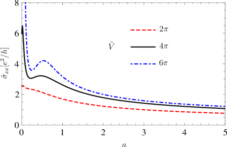
Figure 9: Conductivity $\tilde{\sigma}_{xx}$ for a deformed sinus potential of the form (19) as a function of the deformation parameter $a$ for various potential strengths $\tilde{V}$.

Finally in Fig. 9, we show $\tilde{\sigma}_{xx}$ for the deformed sinus potentials (19) as a function of the deformation parameter $a$ for various potential strengths $\tilde{V}$. We argued in Sect. II that in this case only the central Dirac point exists leading to the fact that $\tilde{\sigma}_{yy}=0$ within the semiclassical approximation. From Fig. 9, we obtain local maxima in $\tilde{\sigma}_{xx}$ at certain deformation values $a$. As can be seen from (31) with (41), these deformation parameters are in a regime where (20) is fulfilled for values of $n\in\mathbb{N}$ and $p_{y}=0$ with ${\rm arg}[\overrightarrow{R}]=-3\pi/4$.

V Success, Failures and possible Applications of the semiclassical approach

Just recently, an extensive analysis of the semiclassical transmission coefficients of np and npn junctions with a comparison to a numerical multistep calculation was carried out Tudorovskiy1 . Up to small deviations for small incident angles of the particles, the authors find quite good agreement of the semiclassical results with their numerics. This is in accordance to the good results we found for the energy spectrum of the (deformed) sinus SL potentials in Sect. II. By taking into account also the good conductivity behavior of the semiclassical approximation described in the last section we could conceive the following application.

As already argued in the introduction of this paper, due to their spectral and conductive properties, electrons in graphene with an overlying SL are interesting systems promising many applications, which could open new routes to building electronic devices. The ability to construct SL potentials which show this behavior for an energy band with desired conduction properties can be very useful. We have shown that this is in principle possible within the semiclassical approximation in our example in Sect. IIB. There we reached the goal to construct SL potentials showing a plateau in the energy spectrum as a function of the transversal momentum using the semiclassical approximation. Unfortunately, this behavior did not survive when calculating the energy spectrum of the constructed SL potential with an exact numerical diagonalization method. The reason lies in the fact that the required smooth behavior of the constructed potential, which is necessary for the validity of the semiclassical approximation was not given. The lesson to be learned from this example is that semiclassically constructed potentials should be further crosschecked by additional means, as e.g. using numerical methods, in order to be trusted.

VI Summary

We have analysed the behavior of electrons in electrical superlattice potentials within a semiclassical approximation. We found this description to work well for smooth superlattice potentials. We started in Sect. IIA by introducing the semiclassical wave function representation of the quasi-relativistic Dirac equation of electrons in graphene superimposed by an SL. We have derived transmission and reflection coefficients for Klein tunneling through a classical forbidden region, in which a particle state is converted to a hole state or vice versa. Within a generalized Bohr-Sommerfeld formalism, we have derived the eigenvalue equations for the lowest energy band of a SL with one electron and one hole region in the fundamental cell, showing only Klein scattering. For electrons in a SL of a (deformed) sinus shape, we obtain very good accordance of the semiclassical energy spectrum with the spectrum obtained by exact numerical diagonalization. Then we tried to construct in Sect. IIB potentials having an energy plateau at zero energy, and uncovered its failure when comparing the semiclassical energy spectrum of the potential with the exact diagonalization method as already described in the last section. In order to pave the path to take into account SLs which are not unidirectional we calculated in Sect. III the semiclassical density of states within the generalized Gutzwiller trace formula by taking into account the beam-splitting extension. Even by considering only small length orbits we could reconstruct the energy spectrum of the lowest band from the density of states maxima. This was carried out explicitly for the (deformed) sinus potential SLs.

Finally we have calculated in Sect. IV longitudinal ballistic conductivities along and transverse to the SL wavevector within the semiclassical approximation. Here we have restricted ourselves again to the simplest point symmetric SLs with one electron and one hole region in the fundamental cell where only Klein scattering is important. We obtain a good quantitative accordance with conductivity curves found in the literature for sinus potentials as a function of the potential strength. In these calculations a transfer matrix method was used in order to calculate the conductivity parallel to the SL wavevector. Furthermore we obtain, as was formerly shown also for step-like SLs, that the conductivity along the wavevector of the SL is mainly governed by electrons in the central valley whereas the orthogonal conductivity is determined mostly by the conductivity contribution of the outermost valley. The contribution of electrons in the central valley is zero in the latter case. In contrast to the step-like SLs, the neglect of the other non-dominant valleys is exponential damped in both cases. This is connected to the fact that the transmission coefficients for Klein tunneling in smooth potentials in contrast to step-like SLs are exponentially small as a function of the length of the classically forbidden region and transversal momentum.

- (1) S. V. Morozov, K. S. Novoselov, M. I. Katsnelson, F. Schedin, D. C. Elias, J. A. Jaszczak, and A. K. Geim, Phys. Rev. Lett. 100, 016602 (2008).
- (2) X. Du, I. Skachko, A. Barker and E. Y. Andrei, Nature Nanotech. 3, 491 (2008).
- (3) K. I. Bolotin, K. J. Sikes, J. Hone, H. L. Stormer, and P. Kim, Phys. Rev. Lett. 101, 096802 (2008).
- (4) H. A. Castro Neto, F. Guinea, N. M. R. Peres, K. S. Novoselov and A. K. Geim, Rev. Mod. Phys. 81, 109 (2009).
- (5) L. Brey and H. A. Fertig, Phys. Rev. Lett. 103, 046809 (2009).
- (6) C.-H. Park, L. Yang, Y.-W. Son, M. L. Cohen, and S. G. Louie, Phys. Rev. Lett. 101, 126804 (2008).
- (7) C.-H. Park, Y.-W. Son, L. Yang, M. L. Cohen, and S. G. Louie, Nano Lett. 8, 2920 (2008).
- (8) M. Yankowitz, J. Xue, D. Cormode, J. D. Sanchez-Yamagishi, K. Watanabe, T. Taniguchi, P. Jarillo-Herrero, P. Jacquod, and B. J. LeRoy, Nat. Phys. 8, 382 (2012).
- (9) C.-H. Park, Y.-W. Son, L. Yang, M. L. Cohen, and S. G. Louie, Phys. Rev. Lett. 103, 046808 (2009).
- (10) V. I. Talyanskii, D. S. Novikov, B. D. Simons, and L. S. Levitov, Phys. Rev. Lett. 87, 276802 (2001).
- (11) M. Barbier, P. Vasilopoulos, and F. M. Peeters, Phys. Rev. B 81, 075438 (2010).
- (12) J. Dietel and H. Kleinert, Phys. Rev. B 86, 115450 (2012).
- (13) C.-H. Park, L. Yang, Y.-W. Son, M. L. Cohen, and S. G. Louie, Nat. Physics 4, 213 (2008).
- (14) J. Dietel and H. Kleinert, Phys. Rev. B 84, 121404(R) (2011).
- (15) P. Burset, A. L. Yeyati, L. Brey, and H. A. Fertig, Phys. Rev. B 83, 195434 (2011).
- (16) M. Barbier, P. Vasilopoulos, F. Peeters, Phil. Trans. R. Soc. A 368, 5499 (2010).
- (17) J. Sun, H. A. Fertig, and L. Brey, Phys. Rev. Lett. 105, 156801 (2010).
- (18) S. -L. Zhu, D. W. Zhang, and Z. D. Wang, Phys. Rev. Lett. 102, 210403 (2009).
- (19) O. Klein, Z. Phys. 53 , 157 (1929).
- (20) A. Hansen and F. Ravndal, Physica Script. 23, 1036 (1981).
- (21) W. Greiner, B. Müller, and J. Rafelski, Quantum Electrodynamics of Strong Fields (Springer, Heidelberg, 1985).
- (22) F. Sauter, Z. Phys. 69, 742 (1931); F. Sauter, Z. Phys. 73, 547 (1931).
- (23) S. I. Rubinow and J. B. Keller, Phys. Rev. 131, 2789 (1963).
- (24) S. Keppeler, Phys. Rev. Lett. 89, 210405 (2002); S. Keppeler, Ann. Phys. (N.Y.), (304), 40 (2003).
- (25) R. G. Littlejohn and W. G. Flynn, Phys. Rev. A 44 5239 (1991).
- (26) V. Maslov and M. V. Fedoriuk, Semi-Classical approximation in quantum mechanics (Reidel, Dodrecht, Netherlands, 1981).
- (27) P. Carmier and D. Ullmo, Phys. Rev. B 77, 245413 (2008).
- (28) M. I. Katsnelson, K. S. Novoselov, and A. K. Geim, Nature Physics 2, 620 (2006).
- (29) C. W. J. Beenackker, Rev. Mod. Phys. 80, 1337 (2008):
- (30) M. Lewkowicz, B. Rosenstein, and D. Nghiem, Phys. Rev. B 84, 115419 (2011).
- (31) M. Abramowitz and I. Stegun, Handbook of Mathematical Functions (Dover, Publications, 1964).
- (32) V. V. Cheianov and V. I. Fal’ko, Phys. Rev. B 74, 041403(R) (2006).
- (33) E. B. Sonin, Phys. Rev. B bf 79, 195438 (2009).
- (34) T. Tudorovskiy, K. J. A. Reijnders and M. I. Katsnelson, Phys. Scr. TI46, 014010 (2012); K. J. A. Reiijnders, T. Tudorovskiy, and M. I. Katsnelson, Ann. Phys. (N.Y.) 333, 155 (2013).
- (35) H. Kleinert, Path integrals in Quantum Mechanics, Statistics, Polymer Physics, and Financial Markets, (World Scientific, London, 2009).
- (36) H. Kosaka, T. Kawashima, A. Tonita, M. Notomi, T. Tamamura, T. Sato, and S. Kawakami, Appl. Phys. Lett. 74, 1212 (1999).
- (37) P. T. Rakich, M. S. Dahlem, S. Tandon, M. Ibanecu, M. SolajaC̆ić, G. S. Petrich, J. D. Joannopoulos, L. A. Kolodiejski, and E. P. Ippen, Nat. Mat. 5, 93 (2006).
- (38) V. Brack and R. K. Bhaduri, Semiclassical Physics (Addison-Wesley, Reading, Massachusetts, 1997).
- (39) M. C. Gutzwiller, J. Math. Phys. 12, 343 (1970).
- (40) J. Bolte and S. Keppeler, Phys. Rev. Lett. 81, 1987 (1998); J. Bolte and S. Keppeler, Annals of Physics 274, 125 (1999).
- (41) L. Couchman, E. Ott and T. M. Antonsen, Jr., Phys. Rev. A, 46, 6193 (1992).
- (42) Y. Dabaghian, R. V. Jensen and R. Blümel, Phys. Rev E, 63, 066201, (2001).
- (43) Y. Dabaghian and R. V. Jensen, EPJ B 26, 423 (2005).
- (44) T. K. Timberlake, Phys. Rev. E 81, 046207 (2010).
- (45) T. Kottos and U. Smilansky, Ann. Phys. 274, 76 (1999).
- (46) M. Lewkowicz and B. Rosenstein, Phys. Rev. Lett. 102, 106802 (2009); H. C. Kao, M. Lewkowicz, and B. Rosenstein Phys. Rev. B 82, 035406 (2010).
- (47) K. Ziegler, Phys. Rev. B 75, 233407 (2007).
- (48) S. Ryu, C. Mudry, A. Furusaki, and A. W. W. Ludwig, Phys. Rev. B. 75, 205344 (2007).
- (49) M. I. Katsnelson, Eur. Phys. J. B 51, 157 (2006).
- (50) J. Tworzydlo, B. Trauzettel, M. Titov, A. Rycerz, and C. W. J. Beenakker, Phys. Rev. Lett. 96, 246802 (2006).