Learning based Channel Load Measurement in 802.11 Networks

Abstract

It is known that load-unaware channel selection in 802.11 networks results in high interference, which can significantly reduce network throughput. In current implementations, the only way to determine traffic load on a channel is to measure the channel. Therefore, in order to find the channel with the minimum load, all channels have to be measured, which is costly and may cause unacceptable communication interruptions between the Access Point (AP) and the stations (STA). In this paper, we propose a learning based approach which seeks the channel with the minimum load by measuring only a limited number of channels. Our method uses Gaussian Process Regressing to accurately track the traffic load on each channel based on previous measured load. We confirm the performance of our approach using experimental data, and show that the time used for the load measurement can be reduced more than 50 $\%$ compared to the case where all channels are monitored.

I Introduction

It is estimated that more than 60% of global Internet traffic will be transmitted over IEEE 802.11 based Wireless Local Area Networks (WLANs) in 2018 [1], bringing high density unstructured networks. Hence, industry efforts such as the IEEE 802.11ac standard are focussed on very high throughput. Moreover the High-Efficiency WLAN (HEW) Study Group [2] is currently working on a new high-throughput amendment named IEEE 802.11ax-2019 which aims to improve user experience especially in dense deployment scenarios. Under such scenarios with high interference levels, identifying the channel with the least traffic load is crucial.

In practical implementations, the traffic load on a particular channel (i.e., channel load) is measured using the Clear Channel Assessment (CCA) mechanism which can measure the fraction of time in which the channel is busy or idle [3]. Acquisition of the channel load information has been standardized with the IEEE 802.11k standard [4], where measurements are performed with request/response frame exchanges. Specifically, by sending a channel load request frame, an AP or STA can request another AP or STA to measure the load of a particular set of channels using CCA. Then, the station that measured the channels returns the channel busy fraction on those channels by sending a channel load report frame.

We note that CCA based load measurement may take significant time since the monitoring station should halt its transmission/reception for the duration of the measurement. To give an idea of how much time is needed to collect load information of each channel, we consider the 5 GHz frequency band where there are 23 non-overlapping channels with a bandwidth of 20 MHz. If a channel is monitored for a duration of 50 milliseconds (ms) then the total time spent for the monitoring process will equal 1150 ms (1.15 seconds), which can significantly degrade the performance of the monitoring station in terms of both the throughput and delay. If the monitoring station is the AP, then the effect of the monitoring becomes more significant.

One way to reduce the overhead of the load measurement is to decrease the measurement time. However, the confidence of each measurement is important parameter since a channel is measured for only a limited time. In [5], it was shown that the measurement duration must be sufficiently large for a certain level of confidence to be guaranteed. In [6], the authors studied the optimization of the duration of a single load measurement. It was shown in [7] that there is significant variation in channel loads reported by the same station at different times, which may have significant effect on the selection of the channel with the minimum load. In [8], the authors proposed a channel selection mechanism which takes into account the channel load without considering the cost of obtaining the load information.

Another approach to reducing the time spent on load measurement is to monitor only a limited number of channels at each measurement time instead of monitoring all channels, which is the approach considered in this paper. Specifically, we propose a dynamic load acquisition algorithm which aims to determine the channel with the minimum traffic load without measuring all channels in the frequency band of interest. Our algorithm is based on the Gaussian Process Regression (GPR) technique [9], which is used to estimate the instantaneous load of each channel by utilizing the previous load measurements. Based on the estimated load and the level of uncertainty in the estimations, it constructs a set of channels to be measured, and only those channels are measured at each measurement time. We show that GPR-based load measurement works well for reducing the cost associated with channel monitoring.

II System Model

We first describe our testbed to collect traffic load experimentally. In our testbed, we use a Wi-Fi device as a measuring station equipped with a Broadcom 802.11n chipset. Although the card does not support 802.11k, it still enables us to measure load using the CCA mechanism, and we examine the traffic load from the wireless driver of the device. We recall that CCA is a function which senses the wireless medium. The channel measurement period is denoted $T$. We note that $T$ depends on the algorithm implemented on the device, and can be modified by end-users. In practice, the channel measurement is performed in a discrete way. Specifically, $T$ is divided into mini-slots of fixed duration, which cannot be changed by end-users (i.e., depends on the card clock). The CCA mechanism returns a 1 if the channel is busy during that mini-slot and otherwise it returns a 0. Let $n(T)$ be the number of mini-slots when the measurement duration is set to $T$. Then, the fraction of busy time of a channel is determined by averaging the results obtained with $n(T)$ samples. As $T$ increases, the number of samples (i.e., mini-slots) increase as well, and the measurements become more accurate.

II-A An Exhaustive Algorithm

Let $\mathcal{C}_{a}=\{C_{1},C_{2},\cdots,C_{M}\}$ be the set of all available channels in the operating frequency band, and $L(t)=\{L_{(}t),L_{2}(t),\cdots,L_{M}(t)\}$ be the traffic load vector where $L_{n}(t)$ represents the traffic load on channel $n$ when the measurements starts at time $t$. We assume that each channel is measured for a duration of $T$ seconds. To gather the load information from all channels, Algorithm 1 is applied, which is an exhaustive algorithm that measures all the available channels in the frequency band of interest.

• Step 1: The monitoring station (MS) receives the measurement request for a duration of $T$ seconds. The request may come from another station or AP.

• Step 2: When the MS starts the measurements:

  • Step 2.1: First, the MS halts its transmission/reception, and measures the load on each channel in $\mathcal{C}_{a}$ for $T$ seconds using CCA.

  • Step 2.2: Then, the MS reports this information back to the AP.

• Step 3: Let $k_{1}^{*}(t)$ be the channel with the minimum load at measurement time $t$.

  $$k_{1}^{*}(t)=\operatornamewithlimits{argmin}_{n\in\mathcal{C}_{a}}L_{n}(t)$$

Algorithm 1 Exhaustive Load Measurement

Let $L_{k_{1}^{*}(t)}$ be the load on channel $k_{1}^{*}(t)$ selected by Algorithm 1 at measurement time $t$. Then, the average channel load using Algorithm 1 is given as,

$$L_{1}=\lim_{t\rightarrow\infty}\frac{1}{t}\sum_{\tau=0}^{t-1}L_{k_{1}^{*}(\tau)}$$ (1)

Let $c_{1}$ be the cost in terms of time consumed with Algorithm 1. Since all the channels are measured by Algorithm 1, $c_{1}=T\times M$.

The cost of employing Algorithm 1 is non-negligible since it requires the MS to monitor a large number of channels for a non-negligible duration. We recall that the following options are available to reduce the time spent for the measurement process: i) decrease $T$, and then the overall time spent for monitoring all channels will be reduced as well. However, as we show in our experimental results given in Section IV, channel selection with small values of $T$ may result in incorrect decisions, and the required confidence level may not be satisfied [5]; ii-) measure only a channel subset instead of all channels.

In our work, we adopt the second solution, and consider that at most $K$ channels can be monitored at a measurement request, where $KM$. We define $\mathcal{C}_{l}(t)$ as the set of channels monitored at measurement time $t$, where $\mid\mathcal{C}_{l}(t)\mid=K$ for all $t$. Recall that when all channels are measured as in Algorithm 1, the channel with the minimum load is guaranteed to be selected. However, when $K$ channels are monitored, it is not guaranteed to find the channel with the minimum traffic load. Hence, it is important to determine the set of channels that should be monitored. Note that the instantaneous measured data may be outdated at the time of channel selection due to the fast variation of the load processes. By taking this into account, in this work we adopt an estimation based solution for the determination of the set of channels, where we predict the instantaneous average of the load process at each measurement time.

III Channel Load Estimation with GPR

We employ GPR for channel load estimation [9]. GPR is a popular learning method for predicting and tracking of continuous processes, and it is widely used especially for practical problems including global optimization [10], wireless scheduling [11], global positioning [12] and estimation in wireless sensor networks [13]. Note that the foundation of GPR is Bayesian inference, where the main idea is to choose an a priori model and update this model with observed measurements. GPR is a suitable approach for the following reasons; i-) GPR is a nonparametric regression model, and the current state of the underlying process can be estimated using only some previous measurement samples; ii-) GPR provides a simple way to measure the uncertainty in the estimation for any given set of channel load measurements. This is particularly important for systems where only limited measurement data exists. ; ii-) Note that the channel load process may be highly non-stationary. GPR can give estimations for the current state of the process using only the most recent measurement results, and this is especially important for non-stationary processes, since previous measurements may become outdated and may not give accurate information about the current state.

Recall that GPR aims to reconstruct the underlying function with limited data, which in our case is the traffic load process. It is important to highlight that the performance of GPR highly depends on how smooth the underlying function is. From our experimental data, we observe that the difference between even two consecutive measurements can be very high, which prevents us from obtaining a smooth function for GPR to work well. In order to make the traffic load process smoother, we employ a linear smoother which uses the moving average by using the most recent $w$ instantaneous load measurements. Specifically, let $\mathcal{D}_{n}(t)=(\textbf{L}_{n}^{a},\boldsymbol{\tau}_{n})$ denote the set of channel load measurements taken in channel $n$ at the beginning of measurement period $t$, where $\textbf{L}_{n}^{a}=\{L_{n_{1}}^{a},L_{n_{2}}^{a},\dots,L_{n_{w}}^{a}\}$ denotes the set of the averaged traffic load using the latest $w$ instantaneous channel load measurements at times, $\boldsymbol{\tau}_{n}=\{\tau_{n}^{1},\tau_{n}^{2},\dots,\tau_{n}^{w}\}$, and $\tau_{n}^{i}<t$, $\forall\tau_{n}^{i}\in\boldsymbol{\tau}_{n}$, $i\in\{1,2,\dots,w\}$.

$$i^{*}=\operatornamewithlimits{argmax}_{1\leq n\leq N}I_{n}(t)=\operatornamewithlimits{argmax}_{1\leq n\leq N}v_{n}(t).$$ (2)

Here, we define the instantaneous average load of a channel at time $t$ as the sample average of the latest $w$ measurements taken until time $t$, where the value of $w$ depends on how fast the measurement statistics change on the channel. We use GPR to determine $\hat{L}_{n}(t)$ given $\mathcal{D}_{n}(t)$ instead of simply averaging the latest $w$ measurements.

The following lemma is similar to the one given in [10], and establishes that the information obtained by probing a channel is equal to the variance of the estimate of the state of that channel.

Lemma 1

Given $\mathcal{D}_{n}(t),\forall n=1,\ldots,N$, finding the channel that gives the best information at time slot $t$ is equal to finding the channel which has the highest variance at that time slot, i.e.,

$$i^{*}=\operatornamewithlimits{argmax}_{1\leq n\leq N}I_{n}(t)=\operatornamewithlimits{argmax}_{1\leq n\leq N}v_{n}(t).$$ (3)

Let $p(L_{n}(t)|t,\mathcal{D}_{n}(t))$ be a posterior distribution of channel $n$. According to GPR, a posterior distribution is Gaussian with mean $\hat{L}_{n}(t)$ and variance $v_{n}(t)$. Specifically, the Gaussian process is specified by the kernel function, $k_{n}(\tau_{n}^{i},\tau_{n}^{j})$, that describes the correlation of the load on channel $n$ between two measurements taken at times $\tau_{n}^{i}$ and $\tau_{n}^{j}$. It is possible to choose any positive definite kernel function. However, the most widely used is the squared exponential, i.e., Gaussian, kernel:

$$k_{n}(\tau_{n}^{i},\tau_{n}^{j})=\exp\left[-\frac{1}{2}(\tau_{n}^{i}-\tau_{n}^{j})^{2}\right].$$ (4)

Given $\mathcal{D}_{n}(t)$, $\hat{L}_{n}(t)$ and variance $v_{n}(t)$ are determined as follows:

$$\hat{L}_{n}(t) =\textbf{k}_{n}^{T}(t)\textbf{K}_{n}^{-1}\textbf{L}_{n},$$ (5)

$$v_{n}(t) =k_{n}(t,t)-\textbf{k}_{n}^{T}(t)\textbf{K}_{n}^{-1}\textbf{k}_{n}(t),$$ (6)

where $\textbf{K}_{n}$ is a $w\times w$ matrix composed of elements $k_{n}(\tau_{n}^{i},\tau_{n}^{j})$ for $1\leq i,j\leq w$ and $\textbf{k}_{n}(t)$ is a vector with elements $k(\tau_{n}^{i},t)$ for $\forall\tau_{n}^{i}\in\boldsymbol{\tau}_{n}$. Hence, the AP can easily predict the load on each channel at time $t$ by using (5). Furthermore, the variance $v_{n}(t)$ is used to measure the level of uncertainty in the estimation.

Note that an estimation cannot be done without some level of uncertainty. The degree of uncertainty in the estimation of the current process highly depends on the previously gathered measurement data and the dynamics of the process. For instance, the uncertainty level in the estimation of the current state of the channel which was monitored recently is less than the channel which has not been measured for a long time. Similar to the work in [10], we use $v_{n}(t)$ as the degree of the uncertainty in the estimation of the channel load. We have two objectives; the first is to minimize the channel load. The second is to measure each channel closely and to acquire as much information about the current load levels of the channels as possible so that the estimation variance,$v_{n}(t)$, is minimized. Next, we introduce our algorithm that aims to meet these two objectives concurrently.

III-A Channel Selection Algorithm with GPR

Here, we propose our algorithm that selects $K$ channels at every measurement time.

• Step 1: The AP receives the latest $w$ load measurements for each channel in $\mathcal{C}(t)$. Then, for each channel the AP:

  • Step 2.1: Calculates $\hat{L}_{n}(t)$ and $v_{n}(t)$ according to (5) and (6). The AP assigns a weight for each channel as follows:

    $$W_{n}(t)=v_{n}(t)\hat{L}_{n}(t)$$

  • Step 2.2: Sorts $W_{n}(t)$ in descending order.

  • Step 2.3: Pick the first $K$ channels in the set denoted $\mathcal{C}_{l}(t)$ .

• Step 3: Then, the AP requests the MS to monitor the channels in set $\mathcal{C}_{l}(t)$.

• Step 4: Let $m(t)$ be the current operating channel of the AP when the load measurement is requested.

  $$k_{2}^{*}(t)=\operatornamewithlimits{argmin}_{n\in\mathcal{C}_{l}(t)}L_{n}(t)$$

• Step 5: If $m(t)\neq k_{2}^{*}(t)$, the AP switches to channel $k_{2}^{*}(t)$, otherwise it continues operating on channel $m(t)$.

Algorithm 2 Channel Load Measurement with GPR

Let $L_{k_{2}^{*}(t)}$ be the load on channel $k_{2}^{*}(t)$ selected by Algorithm 2 at measurement time $t$. Then, the average channel load with Algorithm 2 is given as,

$$L_{2}=\lim_{t\rightarrow\infty}\frac{1}{t}\sum_{\tau=0}^{t-1}L_{k_{2}^{*}(\tau)}$$ (7)

Let $c_{2}$ be the cost in terms of time consumed for monitoring $K$ channels with Algorithm 2, and $c_{2}=T\times K$.

IV Simulation Results

In this section, we provide the results of the impact of $T$ on channel selection, and of the performance assessment of Algorithm 2 in terms of $L_{1}$, $L_{2}$, $c_{1}$ and $c_{2}$. Our tests are carried out at the AirtTies office for the 2.4 GHz band where there are 13 channels with 20 MHz bandwidth (i.e., $M=13$).

IV-A Effect of Measurement duration, $T$

In this part, we investigate the possible effects of the measurement duration $T$ on the performance of a channel selection algorithm. For this, we have conducted various channel load measurements for different values of $T$. During the measurements there were about 10 APs serving more than 50 people. The majority of the APs are of type AirTies 4420 with Broadcom 4717 chipsets where the IEEE 802.11n standard is supported.

The Broadcom 4717 chipsets do not support the request/response frames of 802.11k for measurements, but they are capable of using CCA which allows us to obtain the channel load information.

In our first test, the CCA supporting AP monitors each channel for a duration of 10 ms to gather the load information. The measurements are performed in a consecutive cyclic manner where the AP first measures channel 1, then channel 2 up to channel 13 and then immediately starts over for a total of 50 samples per channel.

Figure 1: Channel load measurements when $T=10$ ms.

Figure 1 shows the channel load measured when $T=10$ ms. For clarity we only plot the results for channel 1 channel 5 and channel 13 as we observe that the other channels show similar characteristics. It can be observed that the variations in the traffic load is high for all channels, which indicates that the load process is non-stationary when $T=10$ ms. The effect of this behavior of the load process leads to proneness for erroneous channel selection. For instance, in Figure 1 we have highlighted sample 8. At this point if the AP monitors the spectrum for channel selection, it observes that the load on channel 1 and channel 5 are equal to 0.77 whereas it is equal to 0.46 for channel 13. Based on this information, the AP decides to operate on channel 13. However, at the next sample point the load on channel 1, channel 5 and channel 13 are 0.09, 0.66 and 0.51 respectively. Hence, at point 9 the best channel with the minimum load is channel 1 and not channel 13. Also, monitoring each channel for an insufficient duration may cause frequent channel switching, which brings additional costs in terms of increased switching delay and frequent user disassociation. Hence, it is important to monitor each channel for a duration large enough so that a sufficient number of samples, $n(T)$, can be obtained, and the average of the obtained samples gives accurate results.

Taking this into account, we repeat the experiment with larger values of $T$. Figure 2 depicts the channel load gathered when $T=50$ ms and $T=100$ ms. Clearly, as $T$ increases the load curves smoothens out and the non-stationarity level decreases, thus, the problems associated with the non-stationary nature of the load process can be mitigated. Next, we present the performance of Algorithm 2 using the load data gathered when $T=100$ ms.

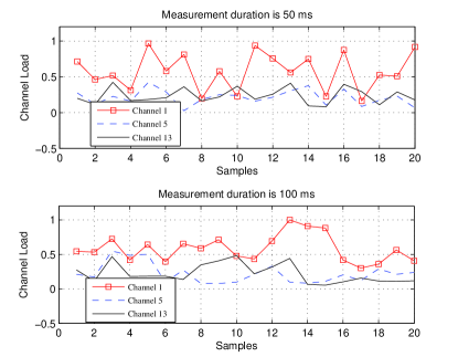
Figure 2: Channel load measurements when $T=50$ and $T=100$ ms.

IV-B Performance of Algorithm 2

In this part, we present the results of the performance assessment of GPR in reducing measurement cost. For this, we apply Algorithm 2 and compare it with Algorithm 1 where all channels are monitored at each measurement time. We also compare Algorithm 2 with a benchmark algorithm which gives the estimation of the instantaneous average of a channel load by averaging the latest $w$ measurement samples.

Figure 3 depicts $L_{1}$ and $L_{2}$ which are the channel load averaged over 50 measurement points after Algorithm 1 and Algorithm 2 are applied, respectively. For Algorithm 2, we change $K$ from $K=2$ to $K=10$, and set $w=2$. Algorithm 1 always selects the channel with the minimum load at each point, and the average channel load is approximately 0.2163, i.e., $L_{1}=0.063$. Clearly, as $K$ increases, the average estimated channel load using Algorithm 2, $L_{2}$ decreases since the accuracy of the estimation increases with GPR, as it tracks the load process well with larger values of $K$. When $K=7$, we observe that $L_{2}$ is approximately equal to 0.065. This means Algorithm 2 can achieve 96 $\%$ of the performance of Algorithm 1 by only monitoring $K=8$ channels. On the other hand, the monitoring cost $c_{1}$ is equal to $13\times 100=1300$ ms whereas $c_{2}$ is equal to $7\times 100=700$ ms. Hence, approximately 54 $\%$ of the cost can be reduced using Algorithm 2 in this scenario.

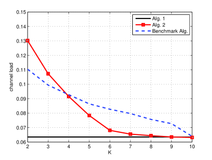
Figure 3: Performance of Algorithm 2 with different values of $K$

In Figure 3, the benchmark algorithm achieves better performance when $K<4$. However when $K>4$, Algorithm 2 outperforms Algorithm 1, which indicates that if $K>4$ the tracking capability of GPR is sufficient to achieve better performance than that of the benchmark algorithm.

Figure 4 depicts the average error in the instantaneous average load estimation when $w=2$, $w=3$ and $w=4$. Clearly, as $K$ increases, the estimation error decreases since the channels are tracked more accurately for higher values of $K$. This experiment indicates that the minimum estimation error is achieved when $w=2$. We conjecture that in this scenario, the channel load measured before the last two measurements is outdated, and it is more beneficial to use the most recent measurement results so that the estimation accuracy of GPR is improved.

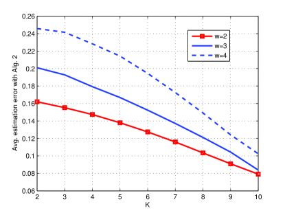
Figure 4: Avg. estimation error with Alg. 2

V Conclusion

We have developed a learning based dynamic channel selection algorithm for the 802.11k supported WLANs. The proposed algorithm has been designed for the channel measurement model where only a limited number of channels are allowed to be monitored at each measurement period. The proposed algorithm first decides on a set of channels that must be monitored, the selection of the operating channel is determined by taking into account the estimated measurement data and the uncertainty levels of each estimation. We apply GPR to predict traffic load on each channel based on previous load measurements. In simulation results, we show that by applying GPR with the proposed algorithm, the cost associated with channel monitoring can be reduced significantly with while only causing a small degradation in performance. In this paper, we assumed that Algorithm 2 takes into account only the uncertainty for channel selection. More efficient algorithms can be developed by both considering the estimated load and the uncertainty, which is our next direction.

References

- [1] Cisco, “The zettabyte era-trends and analysis,” in White Paper, 2014.
- [2] “Webpage, accessed april 2015. [online]. available: http://www.ieee802.org/11/reports/hew update.htm,” IEEE 802.11 Study Group. Status of ieee 802.11 hew study group., 2015.
- [3] P. Dely, A. Kassler, and D. Sivchenko, “Theoretical and experimental analysis of the channel busy fraction in ieee 802.11,” in Future Network and Mobile Summit, 2010.
- [4] IEEE Standard for information technology - Telecommunications and information exchange between sys- tems - Local and metropolitan area networks - Specific requirements Part 11: Wireless LAN Medium Access Control (MAC) and Physical Layer (PHY) Specifications Amendment 1: Radio Resource Measurement of Wireless LANs,, IEEE Std. 802.11k, 2006.
- [5] S. Mangold and L. Berlemann, “IEEE 802.11k: improving confidence in radio resource measurements,” in Proc. 16th IEEE International Symposium on Personal, Indoor and Mobile Radio Communications (PIMR’05), 2005.
- [6] E. A. Panaousis, P. A. Frangoudis, C. N. Ververidis, and G. C. Polyzos, “Optimizing the channel load reporting process in ieee 802.11k-enabled wlans,” in Proc. IEEE LANMAN’08, 2008.
- [7] C. Thorpe, S. Murphy, and L. Murphy, “Analysis of variation in ieee802.11k channel load measurements for neighbouring wlan systems,” in ICT Mobile and Wireless Communications Summit (ICT-MobileSummit’08), Jun. 2008.
- [8] G. Athanasiou1 and L. Tassiulas, “Distributed learning in multi-armed bandit with multiple players,” Transactions on Emerging Telecommunications Technologies, vol. 26, no. 4, pp. 630–649, Apr. 2013.
- [9] C. E. Rasmussen and C. K. I. Williams, Gaussian Processes for Machine Learning (Adaptive Computation and Machine Learning). The MIT Press, 2005.
- [10] T. Alpcan, “A framework for optimization under limited information,” Journal of Global Optimization, 2012.
- [11] M. Karaca, T. Alpcan, and O. Ercetin, “Smart scheduling and feedback allocation over non-stationary wireless channels,” in ICC’12 WS - SCPA, 2012.
- [12] A. Schwaighofer, M. Grigoras, V. Tresp, and C. Hoffmann, “Gpps: A gaussian process positioning system for cellular networks,” in Advances in Neural Information Processing Systems, 2004.
- [13] D. Gu and H. Hu, “Spatial gaussian process regression with mobile sensor networks,” IEEE Trans. Neural Netw. Learn. Syst., vol. 23, no. 8, 2012.