Decomposing CMB lensing power with simulation

Abstract

The reconstruction of the CMB lensing potential is based on a Taylor expansion of lensing effects which is known to have poor convergence properties. For lensing of temperature fluctuations, an understanding of the higher order terms in this expansion which is accurate enough for current experimental sensitivity levels has been developed in Hanson et. al. (2010), as well as a slightly modified Okamoto and Hu quadratic estimator which incorporates lensed rather than unlensed spectra into the estimator weights to mitigate the effect of higher order terms. We extend these results in several ways: (1) We generalize this analysis to the full set of quadratic temperature/polarization lensing estimators, (2) We study the effect of higher order terms for more futuristic experimental noise levels, (3) We show that the ability of the modified quadratic estimator to mitigate the effect of higher order terms relies on a delicate cancellation which occurs only when the true lensed spectra are known. We investigate the sensitivity of this cancellation to uncertainties in or knowledge of these spectra. We find that higher order terms in the Taylor expansion can impact projected error bars at experimental sensitivities similar to those found in future ACTpol/SPTpol experiments.

I Introduction

Over the past year, data from two ground based telescopes, ACT and SPT, have resulted in the first direct measurement of the weak lensing power spectrum solely from CMB measurements Das et al. (2011); van Engelen et al. (2012). In the coming years, the data from Planck and upcoming experiments ACTpol and SPTpol will begin probing this lensing at much greater resolution. The state-of-the-art estimator of weak lensing, the quadratic estimator developed by Hu and Okomoto Hu (2001); Hu and Okamoto (2002), works in part through a delicate cancelation of terms in a Taylor expansion of the lensing effect on the CMB. In this paper we present a simulation based approach for exploring the nature of this cancelation for both the CMB intensity and the polarization fields. In particular, we study a slightly modified quadratic estimator which: incorporates lensed rather than unlensed spectra into the estimator weights to mitigate the effect of higher order terms; and uses the observed lensed CMB fields to correct for the, so called, $N^{(0)}_{\bm{l}}$ bias.

The simulation methodology presented here allows a stochastic exploration of the higher order bias terms of the quadratic estimate and can be used to reduce the computational load associated with iterative de-biasing algorithms for the quadratic estimate. In this paper, we use our simulation methodology to present a detailed study of the, so called, $N^{(1)}_{\bm{l}}$ and $N^{(2)}_{\bm{l}}$ bias for the full set of quadratic temperature/polarization lensing estimators. The $N^{(1)}_{\bm{l}}$ bias was first explored for the standard flat sky quadratic estimate in Kesden et al. Kesden et al. (2003). For full sky CMB temperature maps, Hanson et al. Hanson et al. (2011) developed an approximation to the higher order bias terms, including $N^{(2)}_{\bm{l}}$, which is accurate enough for current experimental sensitivity levels as well as for the slightly modified quadratic estimator which incorporates lensed rather than unlensed spectra into the estimator weights. We generalize this analysis to the full set of modified quadratic temperature/polarization lensing estimators and demonstrate that, indeed, the lensed spectra weights mitigate the combined higher order bias. However, this mitigation is obtained only by an increase in the magnitude of both $N^{(1)}_{\bm{l}}$ and $N^{(2)}_{\bm{l}}$ to the extent that they nearly cancel. We explore the extent with which this cancelation is sensitive to fiducial uncertainty in the way the lensed spectra weights are computed. We find that, under experimental conditions similar to those in future ACTpol and SPTpol experiments, the $EB$ quadratic estimator is not sensitive to low $l$ fiducial uncertainty whereas the $EE$ and $TE$ are sensitive to the point of degrading inferential power.

The remainder of the paper is organized as follows. In sections II, III and IV we give an overview of the modified quadratic estimate, derive the spectral density of the quadratic estimate in terms of higher order bias terms, and discuss the estimation of the spectral density of the lensing potential. In Section V we present two simulation based methods for estimating the higher order bias terms. The first simulation method works exclusively for estimating $N^{(1)}_{\bm{l}}$, and is mainly used to validate the second algorithm which can produce all higher order terms $N^{(j)}_{\bm{l}}$ for $j\geq 1$. In Section VI we use these methods to study the higher order terms for experimental noise levels similar to those found in future ACTpol and SPTpol experiments. The paper concludes with the Appendix which gives fast Fourier transform (FFT) algorithms for computing the modified quadratic estimate. These algorithms extend the FFT techniques developed in Hu (2001) to the computation of all quadratic normalization constants and provides fast (non-stochastic) algorithms which extend the simulation techniques found in Das et al. (2011) for computing the ‘Gaussian bias’ from the lensed CMB four-point function for all temperature/polarization quadratic estimators.

II The quadratic estimator

The effect of weak lensing is to simply remap the CMB temperature $T(\bm{x})$ and Stokes polarization fields $Q(\bm{x})$ and $U(\bm{x})$ for a flat sky coordinate system $\bm{x}\in\mathbb{R}^{2}$. Up to leading order, the remapping displacements are given by $\nabla\phi(\bm{x})$, where $\phi(\bm{x})$ denotes a lensing potential and is the planar projection of a three dimensional gravitational potential (see Dodelson (2003)). Therefore, for any CMB field $X\in\{T,Q,U\}$ the corresponding lensed field can be written $X(\bm{x}+\nabla\phi(\bm{x}))$. For the remainder of the paper we let

$$\tilde{X}(\bm{x})\equiv X(\bm{x}+\nabla\phi(\bm{x}))+N^{\text{\tiny$X$}}(\bm{x})$$

denote the corresponding lensed CMB field with additive independent experimental noise given by $N^{\text{\tiny$X$}}$ (which includes a beam deconvolution). Using this notation the corresponding lensed $E$ and $B$ modes are given by $\tilde{E}_{\bm{l}}\equiv-\cos(2\varphi_{\bm{l}})\tilde{Q}_{\bm{l}}-\sin(2\varphi_{\bm{l}})\tilde{U}_{\bm{l}}$ and $\tilde{B}_{\bm{l}}\equiv\sin(2\varphi_{\bm{l}})\tilde{Q}_{\bm{l}}-\cos(2\varphi_{\bm{l}})\tilde{U}_{\bm{l}}$ where $X_{\bm{l}}\equiv\int\frac{d^{2}\bm{x}}{2\pi}e^{-i\bm{x}\cdot{\bm{l}}}X(\bm{x})$ (unitary angular frequency) and $\varphi_{\bm{l}}$ denotes the phase angle of frequency ${\bm{l}}$.

For any field $X,Y\in\{T,Q,U,E,B\}$ the spectral density $C^{\text{\tiny$X\!Y$}}_{{\bm{l}}}$ is defined to satisfy $\langle X^{\vphantom{*}}_{\bm{l}}Y_{{\bm{l}}^{\prime}}^{*}\rangle=\delta_{{\bm{l}}-{\bm{l}}^{\prime}}C^{\text{\tiny$X\!Y$}}_{{\bm{l}}}$ where $\delta_{\bm{l}}\equiv\int\frac{d^{2}\bm{x}}{(2\pi)^{2}}e^{i\bm{x}\cdot{\bm{l}}}$. The angled brackets $\langle\cdot\rangle$ denote ensemble averaging (or expected value) over both the CMB fields and the large scale structure given by $\phi$. In addition, we let $\langle\cdot\rangle_{\text{\tiny$X\!Y$}}$ denote expected value with respect to the unlensed CMB fields $T,Q,U,E,B$ and $\langle\cdot\rangle_{\phi}$ denote expected value with respect to large scale structure given by $\phi$. Throughout this paper we stipulate $\phi$ is independent of $T,Q,U,E,B$ which implies: $\langle\cdot\rangle=\langle\langle\cdot\rangle_{\text{\tiny$X\!Y$}}\rangle_{\phi}$. We let $\widetilde{C}^{\text{\tiny$X\!Y$}}_{{\bm{l}}}$ denote the lensed CMB spectral density without experimental noise and let $C^{\text{\tiny$X\!Y$}}_{{\bm{l}},\text{\tiny exp}}\equiv C^{\text{\tiny$X\!Y$}}_{{\bm{l}}}+C^{\text{$N^{X}\!N^{Y}$}}_{\bm{l}}$ and $\widetilde{C}^{\text{\tiny$X\!Y$}}_{{\bm{l}},\text{\tiny exp}}\equiv\widetilde{C}^{\text{\tiny$X\!Y$}}_{{\bm{l}}}+C^{\text{ $N^{X}\!N^{Y}$}}_{\bm{l}}$ denote the corresponding unlensed and lensed spectral densities with the additional experimental noise.

The quadratic estimate, based on two lensed CMB fields $\tilde{X}$ and $\tilde{Y}$, is derived from the following two statements:

$$\bigl{\langle}\tilde{X}^{\phantom{*}}_{{\bm{k}}+{\bm{l}}}\tilde{Y}^{*}_{{\bm{k}}} \bigr{\rangle}_{\text{\tiny$X\!Y$}}\approx\phi^{\phantom{*}}_{\bm{l}}f^{\text{\tiny$X\!Y$}}_{{\bm{l}},{\bm{k}}},\quad\text{when ${\bm{l}}\neq 0$;}$$ (1)

$$\bigl{\langle}\tilde{X}^{\phantom{*}}_{{\bm{k}}+{\bm{l}}}\tilde{Y}^{*}_{{\bm{k}}} \bigr{\rangle}_{\phantom{\text{\tiny$X\!Y$}}}=\delta_{{\bm{l}}}\widetilde{C}^{\text{\tiny$X\!Y$}}_{{\bm{k}},\text{\tiny exp}}$$ (2)

which hold for any $X,Y\in\{T,E,B\}$ and where the coefficients $f^{\text{\tiny$X\!Y$}}_{{\bm{l}},{\bm{k}}}$ are given in the Appendix. Equation (1) approximates the cross frequency correlation (at separation lag ${\bm{l}}$) induced by the nonstationarity in $\tilde{X}$ (when regarding $\phi$ as a fixed nonrandom field). This is derived through a Taylor expansion of the lensing operation for any $X\in\{T,Q,U\}$

$$\tilde{X}(\bm{x})=\delta^{0}X(\bm{x})+\delta^{1}X(\bm{x})+\delta^{2}X(\bm{x})+\cdots$$ (3)

where $\delta^{0}X(\bm{x})\equiv X(\bm{x})+N^{\text{\tiny$X$}}(\bm{x})$, $\delta^{1}X(\bm{x})\equiv\nabla^{a}X({\bm{x}})\nabla_{a}\phi({\bm{x}})$, etc. When $X\in\{E,B\}$ one defines $\delta^{j}E_{\bm{l}}\equiv-\cos(2\varphi_{\bm{l}})\delta^{j}Q_{\bm{l}}-\sin(2\varphi_{\bm{l}})\delta^{j}U_{\bm{l}}$ and $\delta^{j}B_{\bm{l}}\equiv\sin(2\varphi_{\bm{l}})\delta^{j}Q_{\bm{l}}-\cos(2\varphi_{\bm{l}})\delta^{j}U_{\bm{l}}$. Then by expanding $\tilde{X}^{\phantom{*}}_{{\bm{k}}+{\bm{l}}}\tilde{Y}^{*}_{{\bm{k}}}$ with (3), regrouping terms by the order of $\phi$, one obtains $f^{\text{\tiny$X\!Y$}}_{{\bm{l}},{\bm{k}}}\phi_{\bm{l}}=\langle\delta^{1}X_{{\bm{k}}+{\bm{l}}}\delta^{0}Y_{\bm{k}}^{*}\rangle_{\text{\tiny$X\!Y$}}+\langle\delta^{0}X_{{\bm{k}}+{\bm{l}}}\delta^{1}Y_{\bm{k}}^{*}\rangle_{\text{\tiny$X\!Y$}}$ which gives approximation (1). Equation (2), on the other hand, is obtained by treating both the CMB and the large scale structure $\phi$ as random so that $\tilde{X}$, from this viewpoint, is isotropic (but non-Gaussian).

Hu and Okamoto Hu (2001); Hu and Okamoto (2002) used approximations (1) and (2) to construct the optimal quadratic estimate of $\phi$ based on $\tilde{X}$ and $\tilde{Y}$ as follows

$$\hat{\phi}_{\bm{l}}^{\text{\tiny$X\!Y$}}\equiv A^{\text{\tiny$X\!Y$}}_{\bm{l}}\int\frac{d^{2}\bm{k}}{2\pi}g^{\text{\tiny$X\!Y$}}_{\bm{l},\bm{k}\,}\tilde{X}_{\bm{k}+\bm{l}}\tilde{Y}^{*}_{\bm{k}}$$ (4)

where $g^{\text{\tiny$X\!Y$}}_{\bm{l},\bm{k}\,}\equiv 2\pi{f^{\text{\tiny$X\!Y$}}_{{\bm{l}},{\bm{k}}}}[\widetilde{C}^{\text{\tiny X\!X}}_{{\bm{k}}+{\bm{l}},\text{\tiny exp}}\widetilde{C}^{\text{\tiny$Y\!Y$}}_{{\bm{k}},\text{\tiny exp}}]^{-1}$. The normalizing constant $A^{\text{\tiny$X\!Y$}}_{\bm{l}}$ is determined through an unbiased constraint. In particular, using the fact that $f_{{\bm{l}},{\bm{k}}}^{\text{\tiny$X\!Y$}}$ is real we have that $\langle\hat{\phi}^{\text{\tiny$X\!Y$}}_{\bm{l}}\rangle_{\text{\tiny$X\!Y$}}=\phi_{\bm{l}}A_{\bm{l}}^{\text{\tiny$X\!Y$}}\int\frac{d^{2}{\bm{k}}}{(2\pi)^{2}}|g^{\text{\tiny$X\!Y$}}_{{\bm{l}},{\bm{k}}}|^{2}\widetilde{C}^{\text{\tiny X\!X}}_{{\bm{k}}+{\bm{l}},\text{\tiny exp}}\widetilde{C}^{\text{\tiny$Y\!Y$}}_{{\bm{k}},\text{\tiny exp}}$ by equation (1). Then requiring that $\bigl{\langle}\hat{\phi}^{\text{\tiny$X\!Y$}}_{\bm{l}}\bigr{\rangle}=\phi_{\bm{l}}$ determines $A^{\text{\tiny$X\!Y$}}_{\bm{l}}$ as follows

$$A_{\bm{l}}^{\text{\tiny$X\!Y$}}=\Bigl{[}\int\frac{d^{2}{\bm{k}}}{(2\pi)^{2}}|g^{\text{\tiny$X\!Y$}}_{{\bm{l}},{\bm{k}}}|^{2}\widetilde{C}^{\text{\tiny X\!X}}_{{\bm{k}}+{\bm{l}},\text{\tiny exp}}\widetilde{C}^{\text{\tiny$Y\!Y$}}_{{\bm{k}},\text{\tiny exp}}\Bigr{]}^{-1}.$$ (5)

II.1 Lensed versus unlensed weights

There is a small modification to the standard quadratic estimate $\hat{\phi}^{\text{\tiny$X\!Y$}}_{\bm{l}}$ which can mitigate the low $l$ bias (arising from the $N^{(2)}_{\bm{l}}$ term discussed in the next section) when using the observed power $|\hat{\phi}^{\text{\tiny$X\!Y$}}_{\bm{l}}|^{2}$ to estimate $C^{\phi\phi}_{\bm{l}}$. This modified estimate, denoted $\tilde{\phi}^{\text{\tiny$X\!Y$}}_{\bm{l}}$, is obtained by replacing all occurrences of unlensed spectra in $g_{{\bm{l}},{\bm{k}}}^{\text{\tiny$X\!Y$}}$ and $A_{\bm{l}}^{\text{\tiny$X\!Y$}}$ with the corresponding lensed spectra. In particular $\tilde{\phi}^{\text{\tiny$X\!Y$}}_{\bm{l}}$ is defined as

$$\tilde{\phi}_{\bm{l}}^{\text{\tiny$X\!Y$}}\equiv\tilde{A}^{\text{\tiny$X\!Y$}}_{\bm{l}}\int\frac{d^{2}\bm{k}}{2\pi}\tilde{g}^{\text{\tiny$X\!Y$}}_{\bm{l},\bm{k}\,}\tilde{X}_{\bm{k}+\bm{l}}\tilde{Y}^{*}_{\bm{k}}$$ (6)

where $\tilde{A}_{\bm{l}}^{\text{\tiny$X\!Y$}}=\bigl{[}\int\frac{d^{2}{\bm{k}}}{(2\pi)^{2}}|\tilde{g}^{\text{\tiny$X\!Y$}}_{{\bm{l}},{\bm{k}}}|^{2}\widetilde{C}^{\text{\tiny X\!X}}_{{\bm{k}}+{\bm{l}},\text{\tiny exp}}\widetilde{C}^{\text{\tiny$Y\!Y$}}_{{\bm{k}},\text{\tiny exp}}\bigr{]}^{-1}$ and $\tilde{g}^{\text{\tiny$X\!Y$}}_{\bm{l},\bm{k}\,}$ is obtained from $g^{\text{\tiny$X\!Y$}}_{\bm{l},\bm{k}\,}$ by replacing every occurrence of $C^{\text{\tiny$X\!Y$}}_{\bm{l}}$, $C^{\text{\tiny$X\!X$}}_{\bm{l}}$ and $C^{\text{\tiny$X\!X$}}_{\bm{l}}$ with the corresponding lensed spectra ${\widetilde{C}}^{\text{\tiny$X\!Y$}}_{\bm{l}}$, $\widetilde{C}^{\text{\tiny$X\!X$}}_{\bm{l}}$ and ${\widetilde{C}}^{\text{\tiny$Y\!Y$}}_{\bm{l}}$. For example, when $X=Y=T$ one has

$$g^{\text{\tiny$TT$}}_{{\bm{l}},{\bm{k}}}\equiv\frac{{\bm{l}}\cdot[({\bm{k}}+{\bm{l}})C^{\text{\tiny$TT$}}_{{\bm{k}}+{\bm{l}}}-{\bm{k}}C^{\text{\tiny$TT$}}_{{\bm{k}}}]}{\widetilde{C}^{\text{\tiny T\!T}}_{{\bm{k}}+{\bm{l}},\text{\tiny exp}}\widetilde{C}^{\text{\tiny$T\!T$}}_{{\bm{k}},\text{\tiny exp}}};$$

$$\tilde{g}^{\text{\tiny$TT$}}_{{\bm{l}},{\bm{k}}}\equiv\frac{{\bm{l}}\cdot[({\bm{k}}+{\bm{l}})\widetilde{C}^{\text{\tiny$TT$}}_{{\bm{k}}+{\bm{l}}}-{\bm{k}}\widetilde{C}^{\text{\tiny$TT$}}_{{\bm{k}}}]}{\widetilde{C}^{\text{\tiny T\!T}}_{{\bm{k}}+{\bm{l}},\text{\tiny exp}}\widetilde{C}^{\text{\tiny$T\!T$}}_{{\bm{k}},\text{\tiny exp}}}.$$

Notice that the estimate $\tilde{\phi}^{\text{\tiny$X\!Y$}}_{\bm{k}}$ is not normalized to be unbiased. Indeed from equation (1) one has

$$\langle\tilde{\phi}^{\text{\tiny$X\!Y$}}_{\bm{l}}\rangle_{\text{\tiny$X\!Y$}} \approx\phi_{\bm{l}}\underbrace{\Bigl{[}\tilde{A}_{\bm{l}}^{\text{\tiny$X\!Y$}}\int\frac{d^{2}{\bm{k}}}{(2\pi)^{2}}\tilde{g}^{\text{\tiny$X\!Y$}}_{\bm{l},\bm{k}\,}g^{\text{\tiny$X\!Y$}}_{\bm{l},\bm{k}\,}\widetilde{C}^{\text{\tiny X\!X}}_{{\bm{k}}+{\bm{l}},\text{\tiny exp}}\widetilde{C}^{\text{\tiny$Y\!Y$}}_{{\bm{k}},\text{\tiny exp}}\Bigr{]}}_{\equiv B_{\bm{l}}^{\text{\tiny$X\!Y$}}}.$$

III The spectral density of the quadratic estimate

In this section we derive the following all order decomposition of the spectral density of the quadratic estimate

$$\bigl{\langle}\hat{\phi}^{\text{\tiny$X\!Y$}}_{\bm{l}}\hat{\phi}^{\text{\tiny$X\!Y$}^{*}}_{{\bm{l}}^{\prime}}\bigr{\rangle} =\delta_{{\bm{l}}-{\bm{l}}^{\prime}}[C_{\bm{l}}^{\phi\phi}+N^{(0)}_{{\bm{l}}}+N^{(1)}_{{\bm{l}}}+\cdots]$$ (7)

which will then be used, in a subsequent section, to derive the estimation bias for $C_{\bm{l}}^{\phi\phi}$. The first term $N^{(0)}_{\bm{l}}$ is related to the disconnected terms of the lensed CMB four-point function, whereas the higher order terms $N_{{\bm{l}}}^{(j)}$ for $j\geq 1$ are related to the connected terms of the four-point function segmented by the order of $C_{\bm{l}}^{\phi\phi}$. Most of this section focuses on the quadratic estimate $\hat{\phi}^{\text{\tiny$X\!Y$}}$ followed by a brief discussion of the corresponding decomposition for the modified quadratic estimate $\tilde{\phi}^{\text{\tiny$X\!Y$}}$.

Our derivation of the spectral density of $\hat{\phi}^{\text{\tiny$X\!Y$}}_{\bm{l}}$ in the flat sky is similar to the analysis of the full sky trispectrum done in Hanson et al. Hanson et al. (2011). One starts by relating $\langle\hat{\phi}^{\text{\tiny$X\!Y$}}_{\bm{l}}\hat{\phi}^{\text{\tiny$X\!Y$}^{*}}_{{\bm{l}}^{\prime}}\rangle$ to the lensed CMB four-point function by distributing the expected value as follows

$$\langle \hat{\phi}^{\text{\tiny$X\!Y$}}_{\bm{l}}\hat{\phi}^{\text{\tiny$X\!Y$}^{*}}_{{\bm{l}}^{\prime}}\rangle=A_{\bm{l}}^{\text{\tiny$X\!Y$}}A_{{\bm{l}}^{\prime}}^{\text{\tiny$X\!Y$}}$$

$$\times\int\frac{d^{2}{\bm{k}}}{2\pi}\int\frac{d^{2}{\bm{k}}^{\prime}}{2\pi}g^{\text{\tiny$X\!Y$}}_{{\bm{l}},{\bm{k}}\,}g^{\text{\tiny$X\!Y$}}_{{\bm{l}}^{\prime},{\bm{k}}^{\prime}}\bigl{\langle}\widetilde{X}^{\phantom{*}}_{\bm{k}+\bm{l}}\widetilde{Y}^{*}_{{\bm{k}}}\widetilde{X}^{*}_{\bm{k}^{\prime}+{\bm{l}}^{\prime}}\widetilde{Y}_{{\bm{k}}^{\prime}}\bigr{\rangle}.$$ (8)

To decompose (8) one then expands the four-point product term in the above integrand by expanding the lensed CMB Taylor expansion (3) to obtain

$$\bigl{\langle}\widetilde{X}^{\phantom{*}}_{\bm{k}+\bm{l}}\widetilde{Y}^{*}_{{\bm{k}}}\widetilde{X}^{*}_{\bm{k}^{\prime}+\bm{l}^{\prime}}\widetilde{Y}_{{\bm{k}}^{\prime}}\bigr{\rangle} =\underbrace{\sum_{i,j,p,q}\bigl{\langle}\delta^{i}X^{\phantom{*}}_{\bm{k}+\bm{l}}\delta^{j}Y^{*}_{{\bm{k}}}\delta^{p}X^{*}_{\bm{k}^{\prime}+\bm{l}^{\prime}}\delta^{q}Y_{{\bm{k}}^{\prime}}\bigr{\rangle}}_{\shortstack{ \text{\small\it decomposes further into connected } \\ \text{\small\it and disconnected terms}}}$$ (9)

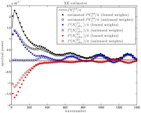
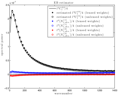
Figure 1: These figures demonstrate the difference between EE and EB quadratic estimators when using lensed versus unlensed spectra into the estimator weights. The main feature of the left hand plot is the reduction of bias—comparing ‘$\ast$’ with ‘$\circ$’—in the EE estimator when the lensed spectra are used for the estimator weights. Also by comparing ‘$\ast$’ with ‘$\circ$’ and ‘$\ast$’ with ‘$\circ$’ it is clear that this reduction is obtained by an increase in magnitude of both the so called $N^{(1)}$ and $N^{(2)}$ bias to extent that they nearly cancel. The first order bias term $l^{4}\bigl{\langle}N^{(1)}_{{\bm{l}},\text{\tiny obs}}\bigr{\rangle}/4$ is denoted ‘$\ast$’ for $\tilde{\phi}^{\text{\tiny$X\!Y$}}_{\bm{l}}$ and ‘$\circ$’ for $\hat{\phi}^{\text{\tiny$X\!Y$}}_{\bm{l}}$. The second order bias term $l^{4}\bigl{\langle}N^{(2)}_{{\bm{l}},\text{\tiny obs}}\bigr{\rangle}/4$ is denoted ‘$\ast$’ for $\tilde{\phi}^{\text{\tiny$X\!Y$}}_{\bm{l}}$ and ‘$\circ$’ for $\hat{\phi}^{\text{\tiny$X\!Y$}}_{\bm{l}}$. Finally, the expected value of the spectral density estimates $l^{4}\langle\delta_{0}^{-1}|\hat{\phi}_{\bm{l}}^{\text{\tiny$X\!Y$}}|^{2}-N^{(0)}_{{\bm{l}},\text{\tiny obs}}\rangle/4$ and $l^{4}\langle\delta_{0}^{-1}|\tilde{\phi}_{\bm{l}}^{\text{\tiny$X\!Y$}}|^{2}-N^{(0)}_{{\bm{l}},\text{\tiny obs}}\rangle/4$ are denoted by ‘$\circ$’ and ‘$\ast$’ respectively. See Section VI for details.

III.1 Disconnected terms

After distributing the expected value in the right hand side of (9) through the $j$-fold convolution which makes up $\delta^{j}X_{\bm{l}}$ and subsequently applying Wicks theorem, one can further decompose $\bigl{\langle}\delta^{i}X^{\phantom{*}}_{\bm{k}+\bm{l}}\delta^{j}Y^{*}_{{\bm{k}}}\delta^{p}X^{*}_{\bm{k}^{\prime}+\bm{l}^{\prime}}\delta^{q}Y_{{\bm{k}}^{\prime}}\bigr{\rangle}$ into what are called connected and disconnected terms. The disconnected terms in the four-point product are the terms which factor into cross-spectra of the fields $\delta^{i}X$, $\delta^{j}X$, $\delta^{p}X$ and $\delta^{q}X$. For example, if $(i,j,p,q)=(1,1,0,0)$ and $\phi$ is assumed independent of $X$ and $Y$ then

$$\bigl{\langle}\delta^{1} X^{\phantom{*}}_{\bm{k}+\bm{l}}\delta^{1}Y^{*}_{{\bm{k}}}\delta^{0}X^{*}_{\bm{k}^{\prime}+\bm{l}^{\prime}}\delta^{0}Y_{{\bm{k}}^{\prime}}\bigr{\rangle}$$

$$=\bigl{\langle}\mathchoice{\vbox{\hbox to0.0pt{\kern 0.0pt\kern 8.72362pt\hbox{\vrule width=0.50003pt,height=0.0pt,depth=4.30554pt\vrule width=17.75974pt,height=0.0pt,depth=0.50003pt\vrule width=0.50003pt,height=0.0pt,depth=4.30554pt}\hss}\vskip 2.15277pt\vskip 8.74889pt}}{\vbox{\hbox to0.0pt{\kern 0.0pt\kern 8.72362pt\hbox{\vrule width=0.50003pt,height=0.0pt,depth=4.30554pt\vrule width=17.75974pt,height=0.0pt,depth=0.50003pt\vrule width=0.50003pt,height=0.0pt,depth=4.30554pt}\hss}\vskip 2.15277pt\vskip 8.74889pt}}{\vbox{\hbox to0.0pt{\kern 0.0pt\kern 5.89653pt\hbox{\vrule width=0.50003pt,height=0.0pt,depth=4.30554pt\vrule width=12.26181pt,height=0.0pt,depth=0.50003pt\vrule width=0.50003pt,height=0.0pt,depth=4.30554pt}\hss}\vskip 2.15277pt\vskip 6.14998pt}}{\vbox{\hbox to0.0pt{\kern 0.0pt\kern 4.54515pt\hbox{\vrule width=0.50003pt,height=0.0pt,depth=4.30554pt\vrule width=9.6632pt,height=0.0pt,depth=0.50003pt\vrule width=0.50003pt,height=0.0pt,depth=4.30554pt}\hss}\vskip 2.15277pt\vskip 4.7611pt}}\mathchoice{\vbox{\hbox to0.0pt{\kern 35.51949pt\kern 9.55693pt\hbox{\vrule width=0.50003pt,height=0.0pt,depth=4.30554pt\vrule width=19.17888pt,height=0.0pt,depth=0.50003pt\vrule width=0.50003pt,height=0.0pt,depth=4.30554pt}\hss}\vskip 2.15277pt\vskip 8.74889pt}}{\vbox{\hbox to0.0pt{\kern 35.51949pt\kern 9.55693pt\hbox{\vrule width=0.50003pt,height=0.0pt,depth=4.30554pt\vrule width=19.17888pt,height=0.0pt,depth=0.50003pt\vrule width=0.50003pt,height=0.0pt,depth=4.30554pt}\hss}\vskip 2.15277pt\vskip 8.74889pt}}{\vbox{\hbox to0.0pt{\kern 24.52362pt\kern 6.72984pt\hbox{\vrule width=0.50003pt,height=0.0pt,depth=4.30554pt\vrule width=13.63928pt,height=0.0pt,depth=0.50003pt\vrule width=0.50003pt,height=0.0pt,depth=4.30554pt}\hss}\vskip 2.15277pt\vskip 6.14998pt}}{\vbox{\hbox to0.0pt{\kern 19.3264pt\kern 5.37846pt\hbox{\vrule width=0.50003pt,height=0.0pt,depth=4.30554pt\vrule width=11.04066pt,height=0.0pt,depth=0.50003pt\vrule width=0.50003pt,height=0.0pt,depth=4.30554pt}\hss}\vskip 2.15277pt\vskip 4.7611pt}}\mathchoice{\lower 2.15277pt\vbox{\hbox to0.0pt{\kern 0.0pt\kern 8.72362pt\hbox{\vrule width=0.50003pt,height=0.0pt,depth=4.30554pt\lower 3.80551pt\hbox{\vrule width=17.75974pt,height=0.0pt,depth=0.50003pt}\vrule width=0.50003pt,height=0.0pt,depth=4.30554pt}\hss}}}{\lower 2.15277pt\vbox{\hbox to0.0pt{\kern 0.0pt\kern 8.72362pt\hbox{\vrule width=0.50003pt,height=0.0pt,depth=4.30554pt\lower 3.80551pt\hbox{\vrule width=17.75974pt,height=0.0pt,depth=0.50003pt}\vrule width=0.50003pt,height=0.0pt,depth=4.30554pt}\hss}}}{\lower 2.15277pt\vbox{\hbox to0.0pt{\kern 0.0pt\kern 5.89653pt\hbox{\vrule width=0.50003pt,height=0.0pt,depth=4.30554pt\lower 3.80551pt\hbox{\vrule width=12.26181pt,height=0.0pt,depth=0.50003pt}\vrule width=0.50003pt,height=0.0pt,depth=4.30554pt}\hss}}}{\lower 2.15277pt\vbox{\hbox to0.0pt{\kern 0.0pt\kern 4.54515pt\hbox{\vrule width=0.50003pt,height=0.0pt,depth=4.30554pt\lower 3.80551pt\hbox{\vrule width=9.6632pt,height=0.0pt,depth=0.50003pt}\vrule width=0.50003pt,height=0.0pt,depth=4.30554pt}\hss}}}{\delta^{1}\!X^{\phantom{*}}_{\bm{k}+\bm{l}}}{\delta^{1}\!Y^{*}_{{\bm{k}}}\,}{\delta^{0}\!X^{*}_{\bm{k}^{\prime}+\bm{l}^{\prime}}\,}{\delta^{0}\!Y_{{\bm{k}}^{\prime}}\,}\bigr{\rangle}\leftarrow\text{\small\it disconnected term}$$

$$\quad+\bigl{\langle}\mathchoice{\vbox{\hbox to0.0pt{\kern 0.0pt\kern 8.72362pt\hbox{\vrule width=0.50003pt,height=0.0pt,depth=8.61108pt\vrule width=55.53168pt,height=0.0pt,depth=0.50003pt\vrule width=0.50003pt,height=0.0pt,depth=8.61108pt}\hss}\vskip 2.15277pt\vskip 8.74889pt}}{\vbox{\hbox to0.0pt{\kern 0.0pt\kern 8.72362pt\hbox{\vrule width=0.50003pt,height=0.0pt,depth=8.61108pt\vrule width=55.53168pt,height=0.0pt,depth=0.50003pt\vrule width=0.50003pt,height=0.0pt,depth=8.61108pt}\hss}\vskip 2.15277pt\vskip 8.74889pt}}{\vbox{\hbox to0.0pt{\kern 0.0pt\kern 5.89653pt\hbox{\vrule width=0.50003pt,height=0.0pt,depth=8.61108pt\vrule width=38.99622pt,height=0.0pt,depth=0.50003pt\vrule width=0.50003pt,height=0.0pt,depth=8.61108pt}\hss}\vskip 2.15277pt\vskip 6.14998pt}}{\vbox{\hbox to0.0pt{\kern 0.0pt\kern 4.54515pt\hbox{\vrule width=0.50003pt,height=0.0pt,depth=8.61108pt\vrule width=31.20038pt,height=0.0pt,depth=0.50003pt\vrule width=0.50003pt,height=0.0pt,depth=8.61108pt}\hss}\vskip 2.15277pt\vskip 4.7611pt}}\mathchoice{\vbox{\hbox to0.0pt{\kern 17.44725pt\kern 9.03612pt\hbox{\vrule width=0.50003pt,height=0.0pt,depth=4.30554pt\vrule width=18.59305pt,height=0.0pt,depth=0.50003pt\vrule width=0.50003pt,height=0.0pt,depth=4.30554pt}\hss}\vskip 2.15277pt\vskip 8.74889pt}}{\vbox{\hbox to0.0pt{\kern 17.44725pt\kern 9.03612pt\hbox{\vrule width=0.50003pt,height=0.0pt,depth=4.30554pt\vrule width=18.59305pt,height=0.0pt,depth=0.50003pt\vrule width=0.50003pt,height=0.0pt,depth=4.30554pt}\hss}\vskip 2.15277pt\vskip 8.74889pt}}{\vbox{\hbox to0.0pt{\kern 11.79308pt\kern 6.36526pt\hbox{\vrule width=0.50003pt,height=0.0pt,depth=4.30554pt\vrule width=13.09512pt,height=0.0pt,depth=0.50003pt\vrule width=0.50003pt,height=0.0pt,depth=4.30554pt}\hss}\vskip 2.15277pt\vskip 6.14998pt}}{\vbox{\hbox to0.0pt{\kern 9.0903pt\kern 5.11804pt\hbox{\vrule width=0.50003pt,height=0.0pt,depth=4.30554pt\vrule width=10.4965pt,height=0.0pt,depth=0.50003pt\vrule width=0.50003pt,height=0.0pt,depth=4.30554pt}\hss}\vskip 2.15277pt\vskip 4.7611pt}}\mathchoice{\lower 2.15277pt\vbox{\hbox to0.0pt{\kern 0.0pt\kern 8.72362pt\hbox{\vrule width=0.50003pt,height=0.0pt,depth=4.30554pt\lower 3.80551pt\hbox{\vrule width=17.75974pt,height=0.0pt,depth=0.50003pt}\vrule width=0.50003pt,height=0.0pt,depth=4.30554pt}\hss}}}{\lower 2.15277pt\vbox{\hbox to0.0pt{\kern 0.0pt\kern 8.72362pt\hbox{\vrule width=0.50003pt,height=0.0pt,depth=4.30554pt\lower 3.80551pt\hbox{\vrule width=17.75974pt,height=0.0pt,depth=0.50003pt}\vrule width=0.50003pt,height=0.0pt,depth=4.30554pt}\hss}}}{\lower 2.15277pt\vbox{\hbox to0.0pt{\kern 0.0pt\kern 5.89653pt\hbox{\vrule width=0.50003pt,height=0.0pt,depth=4.30554pt\lower 3.80551pt\hbox{\vrule width=12.26181pt,height=0.0pt,depth=0.50003pt}\vrule width=0.50003pt,height=0.0pt,depth=4.30554pt}\hss}}}{\lower 2.15277pt\vbox{\hbox to0.0pt{\kern 0.0pt\kern 4.54515pt\hbox{\vrule width=0.50003pt,height=0.0pt,depth=4.30554pt\lower 3.80551pt\hbox{\vrule width=9.6632pt,height=0.0pt,depth=0.50003pt}\vrule width=0.50003pt,height=0.0pt,depth=4.30554pt}\hss}}}{\delta^{1}\!X^{\phantom{*}}_{\bm{k}+\bm{l}}}{\delta^{1}\!Y^{*}_{{\bm{k}}}\,}{\delta^{0}\!X^{*}_{\bm{k}^{\prime}+\bm{l}^{\prime}}\,}{\delta^{0}\!Y_{{\bm{k}}^{\prime}}\,}\bigr{\rangle}\leftarrow\text{\small\it connected term}$$

$$\quad+\bigl{\langle}\mathchoice{\vbox{\hbox to0.0pt{\kern 0.0pt\kern 8.72362pt\hbox{\vrule width=0.50003pt,height=0.0pt,depth=4.30554pt\vrule width=36.3528pt,height=0.0pt,depth=0.50003pt\vrule width=0.50003pt,height=0.0pt,depth=4.30554pt}\hss}\vskip 2.15277pt\vskip 8.74889pt}}{\vbox{\hbox to0.0pt{\kern 0.0pt\kern 8.72362pt\hbox{\vrule width=0.50003pt,height=0.0pt,depth=4.30554pt\vrule width=36.3528pt,height=0.0pt,depth=0.50003pt\vrule width=0.50003pt,height=0.0pt,depth=4.30554pt}\hss}\vskip 2.15277pt\vskip 8.74889pt}}{\vbox{\hbox to0.0pt{\kern 0.0pt\kern 5.89653pt\hbox{\vrule width=0.50003pt,height=0.0pt,depth=4.30554pt\vrule width=25.35693pt,height=0.0pt,depth=0.50003pt\vrule width=0.50003pt,height=0.0pt,depth=4.30554pt}\hss}\vskip 2.15277pt\vskip 6.14998pt}}{\vbox{\hbox to0.0pt{\kern 0.0pt\kern 4.54515pt\hbox{\vrule width=0.50003pt,height=0.0pt,depth=4.30554pt\vrule width=20.15971pt,height=0.0pt,depth=0.50003pt\vrule width=0.50003pt,height=0.0pt,depth=4.30554pt}\hss}\vskip 2.15277pt\vskip 4.7611pt}}\mathchoice{\vbox{\hbox to0.0pt{\kern 17.44725pt\kern 9.03612pt\hbox{\vrule width=0.50003pt,height=0.0pt,depth=8.61108pt\vrule width=37.77193pt,height=0.0pt,depth=0.50003pt\vrule width=0.50003pt,height=0.0pt,depth=8.61108pt}\hss}\vskip 2.15277pt\vskip 8.74889pt}}{\vbox{\hbox to0.0pt{\kern 17.44725pt\kern 9.03612pt\hbox{\vrule width=0.50003pt,height=0.0pt,depth=8.61108pt\vrule width=37.77193pt,height=0.0pt,depth=0.50003pt\vrule width=0.50003pt,height=0.0pt,depth=8.61108pt}\hss}\vskip 2.15277pt\vskip 8.74889pt}}{\vbox{\hbox to0.0pt{\kern 11.79308pt\kern 6.36526pt\hbox{\vrule width=0.50003pt,height=0.0pt,depth=8.61108pt\vrule width=26.7344pt,height=0.0pt,depth=0.50003pt\vrule width=0.50003pt,height=0.0pt,depth=8.61108pt}\hss}\vskip 2.15277pt\vskip 6.14998pt}}{\vbox{\hbox to0.0pt{\kern 9.0903pt\kern 5.11804pt\hbox{\vrule width=0.50003pt,height=0.0pt,depth=8.61108pt\vrule width=21.53719pt,height=0.0pt,depth=0.50003pt\vrule width=0.50003pt,height=0.0pt,depth=8.61108pt}\hss}\vskip 2.15277pt\vskip 4.7611pt}}\mathchoice{\lower 2.15277pt\vbox{\hbox to0.0pt{\kern 0.0pt\kern 8.72362pt\hbox{\vrule width=0.50003pt,height=0.0pt,depth=4.30554pt\lower 3.80551pt\hbox{\vrule width=17.75974pt,height=0.0pt,depth=0.50003pt}\vrule width=0.50003pt,height=0.0pt,depth=4.30554pt}\hss}}}{\lower 2.15277pt\vbox{\hbox to0.0pt{\kern 0.0pt\kern 8.72362pt\hbox{\vrule width=0.50003pt,height=0.0pt,depth=4.30554pt\lower 3.80551pt\hbox{\vrule width=17.75974pt,height=0.0pt,depth=0.50003pt}\vrule width=0.50003pt,height=0.0pt,depth=4.30554pt}\hss}}}{\lower 2.15277pt\vbox{\hbox to0.0pt{\kern 0.0pt\kern 5.89653pt\hbox{\vrule width=0.50003pt,height=0.0pt,depth=4.30554pt\lower 3.80551pt\hbox{\vrule width=12.26181pt,height=0.0pt,depth=0.50003pt}\vrule width=0.50003pt,height=0.0pt,depth=4.30554pt}\hss}}}{\lower 2.15277pt\vbox{\hbox to0.0pt{\kern 0.0pt\kern 4.54515pt\hbox{\vrule width=0.50003pt,height=0.0pt,depth=4.30554pt\lower 3.80551pt\hbox{\vrule width=9.6632pt,height=0.0pt,depth=0.50003pt}\vrule width=0.50003pt,height=0.0pt,depth=4.30554pt}\hss}}}{\delta^{1}\!X^{\phantom{*}}_{\bm{k}+\bm{l}}}{\delta^{1}\!Y^{*}_{{\bm{k}}}\,}{\delta^{0}\!X^{*}_{\bm{k}^{\prime}+\bm{l}^{\prime}}\,}{\delta^{0}\!Y_{{\bm{k}}^{\prime}}\,}\bigr{\rangle}\leftarrow\text{\small\it connected term}$$

where the top contraction symbols correspond to pairing the CMB fields and the bottom contraction symbols correspond to pairing the lensing potential in $\delta^{1}\!X$ and $\delta^{1}\!Y$. The contraction pairings on the above disconnected term results in a product of two spectra as follows

$$\bigl{\langle}\mathchoice{\vbox{\hbox to0.0pt{\kern 0.0pt\kern 8.72362pt\hbox{\vrule width=0.50003pt,height=0.0pt,depth=4.30554pt\vrule width=17.75974pt,height=0.0pt,depth=0.50003pt\vrule width=0.50003pt,height=0.0pt,depth=4.30554pt}\hss}\vskip 2.15277pt\vskip 8.74889pt}}{\vbox{\hbox to0.0pt{\kern 0.0pt\kern 8.72362pt\hbox{\vrule width=0.50003pt,height=0.0pt,depth=4.30554pt\vrule width=17.75974pt,height=0.0pt,depth=0.50003pt\vrule width=0.50003pt,height=0.0pt,depth=4.30554pt}\hss}\vskip 2.15277pt\vskip 8.74889pt}}{\vbox{\hbox to0.0pt{\kern 0.0pt\kern 5.89653pt\hbox{\vrule width=0.50003pt,height=0.0pt,depth=4.30554pt\vrule width=12.26181pt,height=0.0pt,depth=0.50003pt\vrule width=0.50003pt,height=0.0pt,depth=4.30554pt}\hss}\vskip 2.15277pt\vskip 6.14998pt}}{\vbox{\hbox to0.0pt{\kern 0.0pt\kern 4.54515pt\hbox{\vrule width=0.50003pt,height=0.0pt,depth=4.30554pt\vrule width=9.6632pt,height=0.0pt,depth=0.50003pt\vrule width=0.50003pt,height=0.0pt,depth=4.30554pt}\hss}\vskip 2.15277pt\vskip 4.7611pt}}\mathchoice{\vbox{\hbox to0.0pt{\kern 35.51949pt\kern 9.55693pt\hbox{\vrule width=0.50003pt,height=0.0pt,depth=4.30554pt\vrule width=19.17888pt,height=0.0pt,depth=0.50003pt\vrule width=0.50003pt,height=0.0pt,depth=4.30554pt}\hss}\vskip 2.15277pt\vskip 8.74889pt}}{\vbox{\hbox to0.0pt{\kern 35.51949pt\kern 9.55693pt\hbox{\vrule width=0.50003pt,height=0.0pt,depth=4.30554pt\vrule width=19.17888pt,height=0.0pt,depth=0.50003pt\vrule width=0.50003pt,height=0.0pt,depth=4.30554pt}\hss}\vskip 2.15277pt\vskip 8.74889pt}}{\vbox{\hbox to0.0pt{\kern 24.52362pt\kern 6.72984pt\hbox{\vrule width=0.50003pt,height=0.0pt,depth=4.30554pt\vrule width=13.63928pt,height=0.0pt,depth=0.50003pt\vrule width=0.50003pt,height=0.0pt,depth=4.30554pt}\hss}\vskip 2.15277pt\vskip 6.14998pt}}{\vbox{\hbox to0.0pt{\kern 19.3264pt\kern 5.37846pt\hbox{\vrule width=0.50003pt,height=0.0pt,depth=4.30554pt\vrule width=11.04066pt,height=0.0pt,depth=0.50003pt\vrule width=0.50003pt,height=0.0pt,depth=4.30554pt}\hss}\vskip 2.15277pt\vskip 4.7611pt}}\mathchoice{\lower 2.15277pt\vbox{\hbox to0.0pt{\kern 0.0pt\kern 8.72362pt\hbox{\vrule width=0.50003pt,height=0.0pt,depth=4.30554pt\lower 3.80551pt\hbox{\vrule width=17.75974pt,height=0.0pt,depth=0.50003pt}\vrule width=0.50003pt,height=0.0pt,depth=4.30554pt}\hss}}}{\lower 2.15277pt\vbox{\hbox to0.0pt{\kern 0.0pt\kern 8.72362pt\hbox{\vrule width=0.50003pt,height=0.0pt,depth=4.30554pt\lower 3.80551pt\hbox{\vrule width=17.75974pt,height=0.0pt,depth=0.50003pt}\vrule width=0.50003pt,height=0.0pt,depth=4.30554pt}\hss}}}{\lower 2.15277pt\vbox{\hbox to0.0pt{\kern 0.0pt\kern 5.89653pt\hbox{\vrule width=0.50003pt,height=0.0pt,depth=4.30554pt\lower 3.80551pt\hbox{\vrule width=12.26181pt,height=0.0pt,depth=0.50003pt}\vrule width=0.50003pt,height=0.0pt,depth=4.30554pt}\hss}}}{\lower 2.15277pt\vbox{\hbox to0.0pt{\kern 0.0pt\kern 4.54515pt\hbox{\vrule width=0.50003pt,height=0.0pt,depth=4.30554pt\lower 3.80551pt\hbox{\vrule width=9.6632pt,height=0.0pt,depth=0.50003pt}\vrule width=0.50003pt,height=0.0pt,depth=4.30554pt}\hss}}}{\delta^{1}\!X^{\phantom{*}}_{\bm{k}+\bm{l}}}{\delta^{1}\!Y^{*}_{{\bm{k}}}\,}{\delta^{0}\!X^{*}_{\bm{k}^{\prime}+\bm{l}^{\prime}}\,}{\delta^{0}\!Y_{{\bm{k}}^{\prime}}\,}\bigr{\rangle}$$

$$\qquad\qquad\quad=\bigl{\langle}{\delta^{1}\!X^{\phantom{*}}_{\bm{k}+\bm{l}}}{\delta^{1}\!Y^{*}_{{\bm{k}}}\,}\bigr{\rangle}\bigl{\langle}{\delta^{0}\!X^{*}_{\bm{k}^{\prime}+\bm{l}^{\prime}}\,}{\delta^{0}\!Y_{{\bm{k}}^{\prime}}\,}\bigr{\rangle}.$$

In a similar manner, for general $(i,j,p,q)$, the disconnected terms can be grouped into the three types: one for each possible configuration of the of top contraction symbols. Then regrouping all disconnected terms in (9), by top contraction type, results in the following three terms:

$$\text{\small\it disconnected terms in}\sum_{i,j,p,q}\bigl{\langle}\delta^{i}X^{\phantom{*}}_{\bm{k}+\bm{l}}\delta^{j}Y^{*}_{{\bm{k}}}\delta^{p}X^{*}_{\bm{k}^{\prime}+\bm{l}^{\prime}}\delta^{q}Y_{{\bm{k}}^{\prime}}\bigr{\rangle}$$

$$\qquad=\bigl{\langle}\mathchoice{\vbox{\hbox to0.0pt{\kern 0.0pt\kern 4.17778pt\hbox{\vrule width=0.50003pt,height=0.0pt,depth=8.61108pt\vrule width=29.8191pt,height=0.0pt,depth=0.50003pt\vrule width=0.50003pt,height=0.0pt,depth=8.61108pt}\hss}\vskip 2.15277pt\vskip 8.52501pt}}{\vbox{\hbox to0.0pt{\kern 0.0pt\kern 4.17778pt\hbox{\vrule width=0.50003pt,height=0.0pt,depth=8.61108pt\vrule width=29.8191pt,height=0.0pt,depth=0.50003pt\vrule width=0.50003pt,height=0.0pt,depth=8.61108pt}\hss}\vskip 2.15277pt\vskip 8.52501pt}}{\vbox{\hbox to0.0pt{\kern 0.0pt\kern 3.77779pt\hbox{\vrule width=0.50003pt,height=0.0pt,depth=8.61108pt\vrule width=27.37744pt,height=0.0pt,depth=0.50003pt\vrule width=0.50003pt,height=0.0pt,depth=8.61108pt}\hss}\vskip 2.15277pt\vskip 8.15279pt}}{\vbox{\hbox to0.0pt{\kern 0.0pt\kern 3.77779pt\hbox{\vrule width=0.50003pt,height=0.0pt,depth=8.61108pt\vrule width=27.37744pt,height=0.0pt,depth=0.50003pt\vrule width=0.50003pt,height=0.0pt,depth=8.61108pt}\hss}\vskip 2.15277pt\vskip 8.15279pt}}\mathchoice{\vbox{\hbox to0.0pt{\kern 8.35558pt\kern 5.0111pt\hbox{\vrule width=0.50003pt,height=0.0pt,depth=4.30554pt\vrule width=10.0222pt,height=0.0pt,depth=0.50003pt\vrule width=0.50003pt,height=0.0pt,depth=4.30554pt}\hss}\vskip 2.15277pt\vskip 8.52501pt}}{\vbox{\hbox to0.0pt{\kern 8.35558pt\kern 5.0111pt\hbox{\vrule width=0.50003pt,height=0.0pt,depth=4.30554pt\vrule width=10.0222pt,height=0.0pt,depth=0.50003pt\vrule width=0.50003pt,height=0.0pt,depth=4.30554pt}\hss}\vskip 2.15277pt\vskip 8.52501pt}}{\vbox{\hbox to0.0pt{\kern 7.55557pt\kern 4.6111pt\hbox{\vrule width=0.50003pt,height=0.0pt,depth=4.30554pt\vrule width=9.2222pt,height=0.0pt,depth=0.50003pt\vrule width=0.50003pt,height=0.0pt,depth=4.30554pt}\hss}\vskip 2.15277pt\vskip 8.15279pt}}{\vbox{\hbox to0.0pt{\kern 7.55557pt\kern 4.6111pt\hbox{\vrule width=0.50003pt,height=0.0pt,depth=4.30554pt\vrule width=9.2222pt,height=0.0pt,depth=0.50003pt\vrule width=0.50003pt,height=0.0pt,depth=4.30554pt}\hss}\vskip 2.15277pt\vskip 8.15279pt}}{\tilde{X}^{\phantom{*}}_{\bm{k}+\bm{l}}}{\tilde{Y}^{*}_{{\bm{k}}}\,}{\tilde{X}^{*}_{\bm{k}^{\prime}+\bm{l}^{\prime}}\,}{\tilde{Y}_{{\bm{k}}^{\prime}}\,}\bigr{\rangle}+\bigl{\langle}\mathchoice{\vbox{\hbox to0.0pt{\kern 0.0pt\kern 4.17778pt\hbox{\vrule width=0.50003pt,height=0.0pt,depth=4.30554pt\vrule width=19.21109pt,height=0.0pt,depth=0.50003pt\vrule width=0.50003pt,height=0.0pt,depth=4.30554pt}\hss}\vskip 2.15277pt\vskip 8.52501pt}}{\vbox{\hbox to0.0pt{\kern 0.0pt\kern 4.17778pt\hbox{\vrule width=0.50003pt,height=0.0pt,depth=4.30554pt\vrule width=19.21109pt,height=0.0pt,depth=0.50003pt\vrule width=0.50003pt,height=0.0pt,depth=4.30554pt}\hss}\vskip 2.15277pt\vskip 8.52501pt}}{\vbox{\hbox to0.0pt{\kern 0.0pt\kern 3.77779pt\hbox{\vrule width=0.50003pt,height=0.0pt,depth=4.30554pt\vrule width=17.61108pt,height=0.0pt,depth=0.50003pt\vrule width=0.50003pt,height=0.0pt,depth=4.30554pt}\hss}\vskip 2.15277pt\vskip 8.15279pt}}{\vbox{\hbox to0.0pt{\kern 0.0pt\kern 3.77779pt\hbox{\vrule width=0.50003pt,height=0.0pt,depth=4.30554pt\vrule width=17.61108pt,height=0.0pt,depth=0.50003pt\vrule width=0.50003pt,height=0.0pt,depth=4.30554pt}\hss}\vskip 2.15277pt\vskip 8.15279pt}}\mathchoice{\vbox{\hbox to0.0pt{\kern 8.35558pt\kern 5.0111pt\hbox{\vrule width=0.50003pt,height=0.0pt,depth=8.61108pt\vrule width=20.63022pt,height=0.0pt,depth=0.50003pt\vrule width=0.50003pt,height=0.0pt,depth=8.61108pt}\hss}\vskip 2.15277pt\vskip 8.52501pt}}{\vbox{\hbox to0.0pt{\kern 8.35558pt\kern 5.0111pt\hbox{\vrule width=0.50003pt,height=0.0pt,depth=8.61108pt\vrule width=20.63022pt,height=0.0pt,depth=0.50003pt\vrule width=0.50003pt,height=0.0pt,depth=8.61108pt}\hss}\vskip 2.15277pt\vskip 8.52501pt}}{\vbox{\hbox to0.0pt{\kern 7.55557pt\kern 4.6111pt\hbox{\vrule width=0.50003pt,height=0.0pt,depth=8.61108pt\vrule width=18.98856pt,height=0.0pt,depth=0.50003pt\vrule width=0.50003pt,height=0.0pt,depth=8.61108pt}\hss}\vskip 2.15277pt\vskip 8.15279pt}}{\vbox{\hbox to0.0pt{\kern 7.55557pt\kern 4.6111pt\hbox{\vrule width=0.50003pt,height=0.0pt,depth=8.61108pt\vrule width=18.98856pt,height=0.0pt,depth=0.50003pt\vrule width=0.50003pt,height=0.0pt,depth=8.61108pt}\hss}\vskip 2.15277pt\vskip 8.15279pt}}{\tilde{X}^{\phantom{*}}_{\bm{k}+\bm{l}}}{\tilde{Y}^{*}_{{\bm{k}}}\,}{\tilde{X}^{*}_{\bm{k}^{\prime}+\bm{l}^{\prime}}\,}{\tilde{Y}_{{\bm{k}}^{\prime}}\,}\bigr{\rangle}$$

$$\qquad\qquad\qquad\qquad\qquad\qquad\quad\!\!\!+\underbrace{\bigl{\langle}\mathchoice{\vbox{\hbox to0.0pt{\kern 0.0pt\kern 4.17778pt\hbox{\vrule width=0.50003pt,height=0.0pt,depth=4.30554pt\vrule width=9.18889pt,height=0.0pt,depth=0.50003pt\vrule width=0.50003pt,height=0.0pt,depth=4.30554pt}\hss}\vskip 2.15277pt\vskip 8.52501pt}}{\vbox{\hbox to0.0pt{\kern 0.0pt\kern 4.17778pt\hbox{\vrule width=0.50003pt,height=0.0pt,depth=4.30554pt\vrule width=9.18889pt,height=0.0pt,depth=0.50003pt\vrule width=0.50003pt,height=0.0pt,depth=4.30554pt}\hss}\vskip 2.15277pt\vskip 8.52501pt}}{\vbox{\hbox to0.0pt{\kern 0.0pt\kern 3.77779pt\hbox{\vrule width=0.50003pt,height=0.0pt,depth=4.30554pt\vrule width=8.38889pt,height=0.0pt,depth=0.50003pt\vrule width=0.50003pt,height=0.0pt,depth=4.30554pt}\hss}\vskip 2.15277pt\vskip 8.15279pt}}{\vbox{\hbox to0.0pt{\kern 0.0pt\kern 3.77779pt\hbox{\vrule width=0.50003pt,height=0.0pt,depth=4.30554pt\vrule width=8.38889pt,height=0.0pt,depth=0.50003pt\vrule width=0.50003pt,height=0.0pt,depth=4.30554pt}\hss}\vskip 2.15277pt\vskip 8.15279pt}}\mathchoice{\vbox{\hbox to0.0pt{\kern 18.37778pt\kern 5.0111pt\hbox{\vrule width=0.50003pt,height=0.0pt,depth=4.30554pt\vrule width=10.60802pt,height=0.0pt,depth=0.50003pt\vrule width=0.50003pt,height=0.0pt,depth=4.30554pt}\hss}\vskip 2.15277pt\vskip 8.52501pt}}{\vbox{\hbox to0.0pt{\kern 18.37778pt\kern 5.0111pt\hbox{\vrule width=0.50003pt,height=0.0pt,depth=4.30554pt\vrule width=10.60802pt,height=0.0pt,depth=0.50003pt\vrule width=0.50003pt,height=0.0pt,depth=4.30554pt}\hss}\vskip 2.15277pt\vskip 8.52501pt}}{\vbox{\hbox to0.0pt{\kern 16.77777pt\kern 4.6111pt\hbox{\vrule width=0.50003pt,height=0.0pt,depth=4.30554pt\vrule width=9.76636pt,height=0.0pt,depth=0.50003pt\vrule width=0.50003pt,height=0.0pt,depth=4.30554pt}\hss}\vskip 2.15277pt\vskip 8.15279pt}}{\vbox{\hbox to0.0pt{\kern 16.77777pt\kern 4.6111pt\hbox{\vrule width=0.50003pt,height=0.0pt,depth=4.30554pt\vrule width=9.76636pt,height=0.0pt,depth=0.50003pt\vrule width=0.50003pt,height=0.0pt,depth=4.30554pt}\hss}\vskip 2.15277pt\vskip 8.15279pt}}{\tilde{X}^{\phantom{*}}_{\bm{k}+\bm{l}}}{\tilde{Y}^{*}_{{\bm{k}}}\,}{\tilde{X}^{*}_{\bm{k}^{\prime}+\bm{l}^{\prime}}\,}{\tilde{Y}_{{\bm{k}}^{\prime}}\,}\bigr{\rangle}}_{=0\text{ when ${\bm{l}}\neq 0$ or ${\bm{l}}^{\prime}\neq 0$}}$$

$$\qquad=\widetilde{C}^{\text{\tiny X\!Y}}_{{\bm{k}}+{\bm{l}},\text{\tiny exp}}\widetilde{C}^{\text{\tiny X\!Y}}_{{\bm{k}},\text{\tiny exp}}\delta_{{\bm{k}}+{\bm{k}}^{\prime}+{\bm{l}}^{\prime}}\delta_{{\bm{k}}+{\bm{k}}^{\prime}+{\bm{l}}}$$ (10)

$$\qquad\qquad\qquad\qquad+\widetilde{C}^{\text{\tiny X\!X}}_{{\bm{k}}+{\bm{l}},\text{\tiny exp}}\widetilde{C}^{\text{\tiny Y\!Y}}_{{\bm{k}},\text{\tiny exp}}\delta_{{\bm{k}}-{\bm{k}}^{\prime}}\delta_{{\bm{k}}+{\bm{l}}-{\bm{k}}^{\prime}-{\bm{l}}^{\prime}}$$

where the last line is obtained by applying approximation (2). Substituting the four-point product term in (8) with (10) results in, what is typically called, the $N^{(0)}_{\bm{l}}$ bias:

$$\text{\small\it disconnected terms in $\bigl{\langle}\hat{\phi}^{\text{\tiny$X\!Y$}}_{\bm{l}}\hat{\phi}^{\text{\tiny$X\!Y$}^{*}}_{{\bm{l}}^{\prime}}\bigr{\rangle}$}=\delta_{{\bm{l}}-{\bm{l}}^{\prime}}N^{(0)}_{{\bm{l}}}$$

where

$$N^{(0)}_{{\bm{l}}}\equiv[A^{\text{\tiny$X\!Y$}}_{\bm{l}}]^{2}\int\frac{d^{2}{\bm{k}}}{(2\pi)^{2}}\Bigl{(}g^{\text{\tiny$X\!Y$}}_{\bm{l},{\bm{k}}\,}g^{\text{\tiny$X\!Y$}}_{{\bm{l}},-{\bm{k}}-{\bm{l}}\,}\widetilde{C}^{\text{\tiny$X\!Y$}}_{{\bm{k}}+{\bm{l}},\text{\tiny exp}}\widetilde{C}^{\text{\tiny$X\!Y$}}_{{\bm{k}},\text{\tiny exp}}$$

$$+|g^{\text{\tiny$X\!Y$}}_{\bm{l},\bm{k}}|^{2}\widetilde{C}^{\text{\tiny$X\!X$}}_{{\bm{k}}+{\bm{l}},\text{\tiny exp}}\widetilde{C}^{\text{\tiny$Y\!Y$}}_{{\bm{k}},\text{\tiny exp}}\Bigr{)}$$ .

III.2 Connected terms

The connected terms decompose further into what we call the ‘first connected terms’ and the ‘second connected terms’. There are only four ‘first connected terms’ and are defined as follows:

first connected $$\text{\small\it{}terms in}\sum_{i,j,p,q}\bigl{\langle}\delta^{i}X^{\phantom{*}}_{\bm{k}+\bm{l}}\delta^{j}Y^{*}_{{\bm{k}}}\delta^{p}X^{*}_{\bm{k}^{\prime}+\bm{l}^{\prime}}\delta^{q}Y_{{\bm{k}}^{\prime}}\bigr{\rangle}$$

$$\equiv\bigl{\langle}\mathchoice{\vbox{\hbox to0.0pt{\kern 0.0pt\kern 12.7711pt\hbox{\vrule width=0.50003pt,height=0.0pt,depth=4.30554pt\vrule width=21.95305pt,height=0.0pt,depth=0.50003pt\vrule width=0.50003pt,height=0.0pt,depth=4.30554pt}\hss}\vskip 2.15277pt\vskip 8.74889pt}}{\vbox{\hbox to0.0pt{\kern 0.0pt\kern 12.7711pt\hbox{\vrule width=0.50003pt,height=0.0pt,depth=4.30554pt\vrule width=21.95305pt,height=0.0pt,depth=0.50003pt\vrule width=0.50003pt,height=0.0pt,depth=4.30554pt}\hss}\vskip 2.15277pt\vskip 8.74889pt}}{\vbox{\hbox to0.0pt{\kern 0.0pt\kern 9.02568pt\hbox{\vrule width=0.50003pt,height=0.0pt,depth=4.30554pt\vrule width=15.49512pt,height=0.0pt,depth=0.50003pt\vrule width=0.50003pt,height=0.0pt,depth=4.30554pt}\hss}\vskip 2.15277pt\vskip 6.14998pt}}{\vbox{\hbox to0.0pt{\kern 0.0pt\kern 7.6743pt\hbox{\vrule width=0.50003pt,height=0.0pt,depth=4.30554pt\vrule width=12.89651pt,height=0.0pt,depth=0.50003pt\vrule width=0.50003pt,height=0.0pt,depth=4.30554pt}\hss}\vskip 2.15277pt\vskip 4.7611pt}}\mathchoice{\vbox{\hbox to0.0pt{\kern 43.90611pt\kern 9.55693pt\hbox{\vrule width=0.50003pt,height=0.0pt,depth=4.30554pt\vrule width=19.17888pt,height=0.0pt,depth=0.50003pt\vrule width=0.50003pt,height=0.0pt,depth=4.30554pt}\hss}\vskip 2.15277pt\vskip 8.74889pt}}{\vbox{\hbox to0.0pt{\kern 43.90611pt\kern 9.55693pt\hbox{\vrule width=0.50003pt,height=0.0pt,depth=4.30554pt\vrule width=19.17888pt,height=0.0pt,depth=0.50003pt\vrule width=0.50003pt,height=0.0pt,depth=4.30554pt}\hss}\vskip 2.15277pt\vskip 8.74889pt}}{\vbox{\hbox to0.0pt{\kern 30.99025pt\kern 6.72984pt\hbox{\vrule width=0.50003pt,height=0.0pt,depth=4.30554pt\vrule width=13.63928pt,height=0.0pt,depth=0.50003pt\vrule width=0.50003pt,height=0.0pt,depth=4.30554pt}\hss}\vskip 2.15277pt\vskip 6.14998pt}}{\vbox{\hbox to0.0pt{\kern 25.79303pt\kern 5.37846pt\hbox{\vrule width=0.50003pt,height=0.0pt,depth=4.30554pt\vrule width=11.04066pt,height=0.0pt,depth=0.50003pt\vrule width=0.50003pt,height=0.0pt,depth=4.30554pt}\hss}\vskip 2.15277pt\vskip 4.7611pt}}\mathchoice{\lower 2.15277pt\vbox{\hbox to0.0pt{\kern 0.0pt\kern 12.7711pt\hbox{\vrule width=0.50003pt,height=0.0pt,depth=4.30554pt\lower 3.80551pt\hbox{\vrule width=40.69194pt,height=0.0pt,depth=0.50003pt}\vrule width=0.50003pt,height=0.0pt,depth=4.30554pt}\hss}}}{\lower 2.15277pt\vbox{\hbox to0.0pt{\kern 0.0pt\kern 12.7711pt\hbox{\vrule width=0.50003pt,height=0.0pt,depth=4.30554pt\lower 3.80551pt\hbox{\vrule width=40.69194pt,height=0.0pt,depth=0.50003pt}\vrule width=0.50003pt,height=0.0pt,depth=4.30554pt}\hss}}}{\lower 2.15277pt\vbox{\hbox to0.0pt{\kern 0.0pt\kern 9.02568pt\hbox{\vrule width=0.50003pt,height=0.0pt,depth=4.30554pt\lower 3.80551pt\hbox{\vrule width=28.69441pt,height=0.0pt,depth=0.50003pt}\vrule width=0.50003pt,height=0.0pt,depth=4.30554pt}\hss}}}{\lower 2.15277pt\vbox{\hbox to0.0pt{\kern 0.0pt\kern 7.6743pt\hbox{\vrule width=0.50003pt,height=0.0pt,depth=4.30554pt\lower 3.80551pt\hbox{\vrule width=23.4972pt,height=0.0pt,depth=0.50003pt}\vrule width=0.50003pt,height=0.0pt,depth=4.30554pt}\hss}}}{\delta^{1}X_{{\bm{k}}+{\bm{l}}}}{\delta^{0}Y_{\bm{k}}^{*}}{\delta^{1}X^{*}_{{\bm{k}}^{\prime}+{\bm{l}}^{\prime}}}{\delta^{0}Y_{{\bm{k}}^{\prime}}}\bigr{\rangle}$$

$$\qquad\qquad+\bigl{\langle}\mathchoice{\vbox{\hbox to0.0pt{\kern 0.0pt\kern 12.7711pt\hbox{\vrule width=0.50003pt,height=0.0pt,depth=4.30554pt\vrule width=21.95305pt,height=0.0pt,depth=0.50003pt\vrule width=0.50003pt,height=0.0pt,depth=4.30554pt}\hss}\vskip 2.15277pt\vskip 8.74889pt}}{\vbox{\hbox to0.0pt{\kern 0.0pt\kern 12.7711pt\hbox{\vrule width=0.50003pt,height=0.0pt,depth=4.30554pt\vrule width=21.95305pt,height=0.0pt,depth=0.50003pt\vrule width=0.50003pt,height=0.0pt,depth=4.30554pt}\hss}\vskip 2.15277pt\vskip 8.74889pt}}{\vbox{\hbox to0.0pt{\kern 0.0pt\kern 9.02568pt\hbox{\vrule width=0.50003pt,height=0.0pt,depth=4.30554pt\vrule width=15.49512pt,height=0.0pt,depth=0.50003pt\vrule width=0.50003pt,height=0.0pt,depth=4.30554pt}\hss}\vskip 2.15277pt\vskip 6.14998pt}}{\vbox{\hbox to0.0pt{\kern 0.0pt\kern 7.6743pt\hbox{\vrule width=0.50003pt,height=0.0pt,depth=4.30554pt\vrule width=12.89651pt,height=0.0pt,depth=0.50003pt\vrule width=0.50003pt,height=0.0pt,depth=4.30554pt}\hss}\vskip 2.15277pt\vskip 4.7611pt}}\mathchoice{\vbox{\hbox to0.0pt{\kern 43.90611pt\kern 9.55693pt\hbox{\vrule width=0.50003pt,height=0.0pt,depth=4.30554pt\vrule width=19.17888pt,height=0.0pt,depth=0.50003pt\vrule width=0.50003pt,height=0.0pt,depth=4.30554pt}\hss}\vskip 2.15277pt\vskip 8.74889pt}}{\vbox{\hbox to0.0pt{\kern 43.90611pt\kern 9.55693pt\hbox{\vrule width=0.50003pt,height=0.0pt,depth=4.30554pt\vrule width=19.17888pt,height=0.0pt,depth=0.50003pt\vrule width=0.50003pt,height=0.0pt,depth=4.30554pt}\hss}\vskip 2.15277pt\vskip 8.74889pt}}{\vbox{\hbox to0.0pt{\kern 30.99025pt\kern 6.72984pt\hbox{\vrule width=0.50003pt,height=0.0pt,depth=4.30554pt\vrule width=13.63928pt,height=0.0pt,depth=0.50003pt\vrule width=0.50003pt,height=0.0pt,depth=4.30554pt}\hss}\vskip 2.15277pt\vskip 6.14998pt}}{\vbox{\hbox to0.0pt{\kern 25.79303pt\kern 5.37846pt\hbox{\vrule width=0.50003pt,height=0.0pt,depth=4.30554pt\vrule width=11.04066pt,height=0.0pt,depth=0.50003pt\vrule width=0.50003pt,height=0.0pt,depth=4.30554pt}\hss}\vskip 2.15277pt\vskip 4.7611pt}}\mathchoice{\lower 2.15277pt\vbox{\hbox to0.0pt{\kern 0.0pt\kern 12.7711pt\hbox{\vrule width=0.50003pt,height=0.0pt,depth=4.30554pt\lower 3.80551pt\hbox{\vrule width=59.87082pt,height=0.0pt,depth=0.50003pt}\vrule width=0.50003pt,height=0.0pt,depth=4.30554pt}\hss}}}{\lower 2.15277pt\vbox{\hbox to0.0pt{\kern 0.0pt\kern 12.7711pt\hbox{\vrule width=0.50003pt,height=0.0pt,depth=4.30554pt\lower 3.80551pt\hbox{\vrule width=59.87082pt,height=0.0pt,depth=0.50003pt}\vrule width=0.50003pt,height=0.0pt,depth=4.30554pt}\hss}}}{\lower 2.15277pt\vbox{\hbox to0.0pt{\kern 0.0pt\kern 9.02568pt\hbox{\vrule width=0.50003pt,height=0.0pt,depth=4.30554pt\lower 3.80551pt\hbox{\vrule width=42.3337pt,height=0.0pt,depth=0.50003pt}\vrule width=0.50003pt,height=0.0pt,depth=4.30554pt}\hss}}}{\lower 2.15277pt\vbox{\hbox to0.0pt{\kern 0.0pt\kern 7.6743pt\hbox{\vrule width=0.50003pt,height=0.0pt,depth=4.30554pt\lower 3.80551pt\hbox{\vrule width=34.53786pt,height=0.0pt,depth=0.50003pt}\vrule width=0.50003pt,height=0.0pt,depth=4.30554pt}\hss}}}{\delta^{1}X_{{\bm{k}}+{\bm{l}}}}{\delta^{0}Y_{\bm{k}}^{*}}{\delta^{0}X^{*}_{{\bm{k}}^{\prime}+{\bm{l}}^{\prime}}}{\delta^{1}Y_{{\bm{k}}^{\prime}}}\bigr{\rangle}$$

$$\qquad\qquad+\bigl{\langle}\mathchoice{\vbox{\hbox to0.0pt{\kern 0.0pt\kern 12.7711pt\hbox{\vrule width=0.50003pt,height=0.0pt,depth=4.30554pt\vrule width=21.95305pt,height=0.0pt,depth=0.50003pt\vrule width=0.50003pt,height=0.0pt,depth=4.30554pt}\hss}\vskip 2.15277pt\vskip 8.74889pt}}{\vbox{\hbox to0.0pt{\kern 0.0pt\kern 12.7711pt\hbox{\vrule width=0.50003pt,height=0.0pt,depth=4.30554pt\vrule width=21.95305pt,height=0.0pt,depth=0.50003pt\vrule width=0.50003pt,height=0.0pt,depth=4.30554pt}\hss}\vskip 2.15277pt\vskip 8.74889pt}}{\vbox{\hbox to0.0pt{\kern 0.0pt\kern 9.02568pt\hbox{\vrule width=0.50003pt,height=0.0pt,depth=4.30554pt\vrule width=15.49512pt,height=0.0pt,depth=0.50003pt\vrule width=0.50003pt,height=0.0pt,depth=4.30554pt}\hss}\vskip 2.15277pt\vskip 6.14998pt}}{\vbox{\hbox to0.0pt{\kern 0.0pt\kern 7.6743pt\hbox{\vrule width=0.50003pt,height=0.0pt,depth=4.30554pt\vrule width=12.89651pt,height=0.0pt,depth=0.50003pt\vrule width=0.50003pt,height=0.0pt,depth=4.30554pt}\hss}\vskip 2.15277pt\vskip 4.7611pt}}\mathchoice{\vbox{\hbox to0.0pt{\kern 43.90611pt\kern 9.55693pt\hbox{\vrule width=0.50003pt,height=0.0pt,depth=4.30554pt\vrule width=19.17888pt,height=0.0pt,depth=0.50003pt\vrule width=0.50003pt,height=0.0pt,depth=4.30554pt}\hss}\vskip 2.15277pt\vskip 8.74889pt}}{\vbox{\hbox to0.0pt{\kern 43.90611pt\kern 9.55693pt\hbox{\vrule width=0.50003pt,height=0.0pt,depth=4.30554pt\vrule width=19.17888pt,height=0.0pt,depth=0.50003pt\vrule width=0.50003pt,height=0.0pt,depth=4.30554pt}\hss}\vskip 2.15277pt\vskip 8.74889pt}}{\vbox{\hbox to0.0pt{\kern 30.99025pt\kern 6.72984pt\hbox{\vrule width=0.50003pt,height=0.0pt,depth=4.30554pt\vrule width=13.63928pt,height=0.0pt,depth=0.50003pt\vrule width=0.50003pt,height=0.0pt,depth=4.30554pt}\hss}\vskip 2.15277pt\vskip 6.14998pt}}{\vbox{\hbox to0.0pt{\kern 25.79303pt\kern 5.37846pt\hbox{\vrule width=0.50003pt,height=0.0pt,depth=4.30554pt\vrule width=11.04066pt,height=0.0pt,depth=0.50003pt\vrule width=0.50003pt,height=0.0pt,depth=4.30554pt}\hss}\vskip 2.15277pt\vskip 4.7611pt}}\mathchoice{\lower 2.15277pt\vbox{\hbox to0.0pt{\kern 25.54222pt\kern 9.18195pt\hbox{\vrule width=0.50003pt,height=0.0pt,depth=4.30554pt\lower 3.80551pt\hbox{\vrule width=18.73888pt,height=0.0pt,depth=0.50003pt}\vrule width=0.50003pt,height=0.0pt,depth=4.30554pt}\hss}}}{\lower 2.15277pt\vbox{\hbox to0.0pt{\kern 25.54222pt\kern 9.18195pt\hbox{\vrule width=0.50003pt,height=0.0pt,depth=4.30554pt\lower 3.80551pt\hbox{\vrule width=18.73888pt,height=0.0pt,depth=0.50003pt}\vrule width=0.50003pt,height=0.0pt,depth=4.30554pt}\hss}}}{\lower 2.15277pt\vbox{\hbox to0.0pt{\kern 18.05138pt\kern 6.46944pt\hbox{\vrule width=0.50003pt,height=0.0pt,depth=4.30554pt\lower 3.80551pt\hbox{\vrule width=13.19928pt,height=0.0pt,depth=0.50003pt}\vrule width=0.50003pt,height=0.0pt,depth=4.30554pt}\hss}}}{\lower 2.15277pt\vbox{\hbox to0.0pt{\kern 15.3486pt\kern 5.22221pt\hbox{\vrule width=0.50003pt,height=0.0pt,depth=4.30554pt\lower 3.80551pt\hbox{\vrule width=10.60068pt,height=0.0pt,depth=0.50003pt}\vrule width=0.50003pt,height=0.0pt,depth=4.30554pt}\hss}}}{\delta^{0}X_{{\bm{k}}+{\bm{l}}}}{\delta^{1}Y_{\bm{k}}^{*}}{\delta^{1}X^{*}_{{\bm{k}}^{\prime}+{\bm{l}}^{\prime}}}{\delta^{0}Y_{{\bm{k}}^{\prime}}}\bigr{\rangle}$$

$$\qquad\qquad+\bigl{\langle}\mathchoice{\vbox{\hbox to0.0pt{\kern 0.0pt\kern 12.7711pt\hbox{\vrule width=0.50003pt,height=0.0pt,depth=4.30554pt\vrule width=21.95305pt,height=0.0pt,depth=0.50003pt\vrule width=0.50003pt,height=0.0pt,depth=4.30554pt}\hss}\vskip 2.15277pt\vskip 8.74889pt}}{\vbox{\hbox to0.0pt{\kern 0.0pt\kern 12.7711pt\hbox{\vrule width=0.50003pt,height=0.0pt,depth=4.30554pt\vrule width=21.95305pt,height=0.0pt,depth=0.50003pt\vrule width=0.50003pt,height=0.0pt,depth=4.30554pt}\hss}\vskip 2.15277pt\vskip 8.74889pt}}{\vbox{\hbox to0.0pt{\kern 0.0pt\kern 9.02568pt\hbox{\vrule width=0.50003pt,height=0.0pt,depth=4.30554pt\vrule width=15.49512pt,height=0.0pt,depth=0.50003pt\vrule width=0.50003pt,height=0.0pt,depth=4.30554pt}\hss}\vskip 2.15277pt\vskip 6.14998pt}}{\vbox{\hbox to0.0pt{\kern 0.0pt\kern 7.6743pt\hbox{\vrule width=0.50003pt,height=0.0pt,depth=4.30554pt\vrule width=12.89651pt,height=0.0pt,depth=0.50003pt\vrule width=0.50003pt,height=0.0pt,depth=4.30554pt}\hss}\vskip 2.15277pt\vskip 4.7611pt}}\mathchoice{\vbox{\hbox to0.0pt{\kern 43.90611pt\kern 9.55693pt\hbox{\vrule width=0.50003pt,height=0.0pt,depth=4.30554pt\vrule width=19.17888pt,height=0.0pt,depth=0.50003pt\vrule width=0.50003pt,height=0.0pt,depth=4.30554pt}\hss}\vskip 2.15277pt\vskip 8.74889pt}}{\vbox{\hbox to0.0pt{\kern 43.90611pt\kern 9.55693pt\hbox{\vrule width=0.50003pt,height=0.0pt,depth=4.30554pt\vrule width=19.17888pt,height=0.0pt,depth=0.50003pt\vrule width=0.50003pt,height=0.0pt,depth=4.30554pt}\hss}\vskip 2.15277pt\vskip 8.74889pt}}{\vbox{\hbox to0.0pt{\kern 30.99025pt\kern 6.72984pt\hbox{\vrule width=0.50003pt,height=0.0pt,depth=4.30554pt\vrule width=13.63928pt,height=0.0pt,depth=0.50003pt\vrule width=0.50003pt,height=0.0pt,depth=4.30554pt}\hss}\vskip 2.15277pt\vskip 6.14998pt}}{\vbox{\hbox to0.0pt{\kern 25.79303pt\kern 5.37846pt\hbox{\vrule width=0.50003pt,height=0.0pt,depth=4.30554pt\vrule width=11.04066pt,height=0.0pt,depth=0.50003pt\vrule width=0.50003pt,height=0.0pt,depth=4.30554pt}\hss}\vskip 2.15277pt\vskip 4.7611pt}}\mathchoice{\lower 2.15277pt\vbox{\hbox to0.0pt{\kern 25.54222pt\kern 9.18195pt\hbox{\vrule width=0.50003pt,height=0.0pt,depth=4.30554pt\lower 3.80551pt\hbox{\vrule width=37.91776pt,height=0.0pt,depth=0.50003pt}\vrule width=0.50003pt,height=0.0pt,depth=4.30554pt}\hss}}}{\lower 2.15277pt\vbox{\hbox to0.0pt{\kern 25.54222pt\kern 9.18195pt\hbox{\vrule width=0.50003pt,height=0.0pt,depth=4.30554pt\lower 3.80551pt\hbox{\vrule width=37.91776pt,height=0.0pt,depth=0.50003pt}\vrule width=0.50003pt,height=0.0pt,depth=4.30554pt}\hss}}}{\lower 2.15277pt\vbox{\hbox to0.0pt{\kern 18.05138pt\kern 6.46944pt\hbox{\vrule width=0.50003pt,height=0.0pt,depth=4.30554pt\lower 3.80551pt\hbox{\vrule width=26.83856pt,height=0.0pt,depth=0.50003pt}\vrule width=0.50003pt,height=0.0pt,depth=4.30554pt}\hss}}}{\lower 2.15277pt\vbox{\hbox to0.0pt{\kern 15.3486pt\kern 5.22221pt\hbox{\vrule width=0.50003pt,height=0.0pt,depth=4.30554pt\lower 3.80551pt\hbox{\vrule width=21.64134pt,height=0.0pt,depth=0.50003pt}\vrule width=0.50003pt,height=0.0pt,depth=4.30554pt}\hss}}}{\delta^{0}X_{{\bm{k}}+{\bm{l}}}}{\delta^{1}Y_{\bm{k}}^{*}}{\delta^{0}X^{*}_{{\bm{k}}^{\prime}+{\bm{l}}^{\prime}}}{\delta^{1}Y_{{\bm{k}}^{\prime}}}\bigr{\rangle}$$

$$=\delta_{{\bm{l}}-{\bm{l}}^{\prime}}f^{\text{\tiny$X\!Y$}}_{{\bm{l}},{\bm{k}}}f^{\text{\tiny$X\!Y$}}_{{\bm{l}}^{\prime},{\bm{k}}^{\prime}}C_{\bm{l}}^{\phi\phi}.$$

Then, by substituting the four-point product term in (8) with the first connected terms, one gets

$$\text{\small\it first connected terms in}\,\bigl{\langle}\hat{\phi}^{\text{\tiny$X\!Y$}}_{\bm{l}}\hat{\phi}^{\text{\tiny$X\!Y$}^{*}}_{{\bm{l}}^{\prime}}\bigr{\rangle}=\delta_{{\bm{l}}-{\bm{l}}^{\prime}}C_{\bm{l}}^{\phi\phi}.$$ (11)

The remaining connected terms in the four-point product of (8), called ‘second connected terms’, are then re-grouping corresponding to the order of $\phi$. After noticing that any term of order $\phi^{2j+1}$ has expected value zero one obtains the following expansion

second connected terms in $$\bigl{\langle}\hat{\phi}^{\text{\tiny$X\!Y$}}_{\bm{l}}\hat{\phi}^{\text{\tiny$X\!Y$}^{*}}_{{\bm{l}}^{\prime}}\bigr{\rangle}$$

$$=\delta_{{\bm{l}}-{\bm{l}}^{\prime}}\bigl{[}N^{(1)}_{\bm{l}}+N^{(2)}_{\bm{l}}+\cdots\bigr{]}$$

where $N^{(j)}_{\bm{l}}$ is of order $\phi^{2j}$. Putting all disconnected and connected terms together gives the desired expansion (7).

For reasons which will become clear in the next section, we define $N^{(1)}_{\bm{l}}$ in a slightly different, but equivalent, way that extends more naturally to the modified quadratic estimate. In particular, instead of defining $N^{(1)}_{\bm{l}}$ as the as the total contribution of the second connected terms in (8) of order $\phi^{2}$, we define $N^{(1)}_{\bm{l}}$ simply as the total contribution of all connected terms of order $\phi^{2}$ minus $C_{\bm{l}}^{\phi\phi}$.

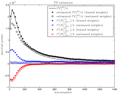
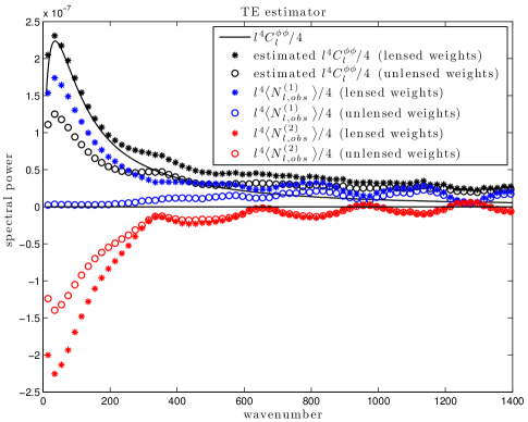
Figure 2: The first order bias term $l^{4}\bigl{\langle}N^{(1)}_{{\bm{l}},\text{\tiny obs}}\bigr{\rangle}/4$ is denoted ‘$\ast$’ for $\tilde{\phi}^{\text{\tiny$X\!Y$}}_{\bm{l}}$ and ‘$\circ$’ for $\hat{\phi}^{\text{\tiny$X\!Y$}}_{\bm{l}}$. The second order bias term $l^{4}\bigl{\langle}N^{(2)}_{{\bm{l}},\text{\tiny obs}}\bigr{\rangle}/4$ is denoted ‘$\ast$’ for $\tilde{\phi}^{\text{\tiny$X\!Y$}}_{\bm{l}}$ and ‘$\circ$’ for $\hat{\phi}^{\text{\tiny$X\!Y$}}_{\bm{l}}$. Finally, the expected value of the spectral density estimates $l^{4}\langle\delta_{0}^{-1}|\hat{\phi}_{\bm{l}}^{\text{\tiny$X\!Y$}}|^{2}-N^{(0)}_{{\bm{l}},\text{\tiny obs}}\rangle/4$ and $l^{4}\langle\delta_{0}^{-1}|\tilde{\phi}_{\bm{l}}^{\text{\tiny$X\!Y$}}|^{2}-N^{(0)}_{{\bm{l}},\text{\tiny obs}}\rangle/4$ are denoted by ‘$\circ$’ and ‘$\ast$’ respectively. See Section VI for details.

III.3 The lensed weights

For the modified quadratic estimator, $\tilde{\phi}^{\text{\tiny$X\!Y$}}_{\bm{l}}$, one can derive the expansion (7) with a few minor adjustments. In particular, the disconnected terms can be written

$$\text{\small\it disconnected terms in $\bigl{\langle}\tilde{\phi}^{\text{\tiny$X\!Y$}}_{\bm{l}}\tilde{\phi}^{\text{\tiny$X\!Y$}^{*}}_{{\bm{l}}^{\prime}}\bigr{\rangle}$}=\delta_{{\bm{l}}-{\bm{l}}^{\prime}}N^{(0)}_{{\bm{l}}}$$

where

$$N^{(0)}_{{\bm{l}}}\equiv[\tilde{A}^{\text{\tiny$X\!Y$}}_{\bm{l}}]^{2}\int\frac{d^{2}{\bm{k}}}{(2\pi)^{2}}\Bigl{(}\tilde{g}^{\text{\tiny$X\!Y$}}_{\bm{l},{\bm{k}}\,}\tilde{g}^{\text{\tiny$X\!Y$}}_{{\bm{l}},-{\bm{k}}-{\bm{l}}\,}\widetilde{C}^{\text{\tiny$X\!Y$}}_{{\bm{k}}+{\bm{l}},\text{\tiny exp}}\widetilde{C}^{\text{\tiny$X\!Y$}}_{{\bm{k}},\text{\tiny exp}}$$

$$+|\tilde{g}^{\text{\tiny$X\!Y$}}_{\bm{l},\bm{k}}|^{2}\widetilde{C}^{\text{\tiny$X\!X$}}_{{\bm{k}}+{\bm{l}},\text{\tiny exp}}\widetilde{C}^{\text{\tiny$Y\!Y$}}_{{\bm{k}},\text{\tiny exp}}\Bigr{)}$$ .

The first connected terms are slightly different due to the intentional bias in the modified quadratic estimate yielding

$$\text{\small\it first connected terms in}\,\bigl{\langle}\tilde{\phi}^{\text{\tiny$X\!Y$}}_{\bm{l}}\tilde{\phi}^{\text{\tiny$X\!Y$}^{*}}_{{\bm{l}}^{\prime}}\bigr{\rangle}=\delta_{{\bm{l}}-{\bm{l}}^{\prime}}[B^{\text{\tiny$X\!Y$}}_{\bm{l}}]^{2}C_{\bm{l}}^{\phi\phi}.$$

After these adjustments are made the remaining terms $N^{(j)}_{\bm{l}}$ are defined exactly the same way as for $\hat{\phi}^{\text{\tiny$X\!Y$}}_{\bm{l}}$: when $j\geq 2$, $N_{\bm{l}}^{(j)}$ is defined as the total contribution of the connected terms in (8) which are order $\phi^{j}$; and $N^{(1)}_{\bm{l}}$ as the total contribution of the connected terms in (8) which are order $\phi^{2}$ minus $C_{\bm{l}}^{\phi\phi}$. This is consistent with the previous definition of $N^{(j)}_{\bm{l}}$ for $\hat{\phi}_{\bm{l}}^{\text{\tiny$X\!Y$}}$ and preserves the natural expansion

$$\bigl{\langle}\tilde{\phi}^{\text{\tiny$X\!Y$}}_{\bm{l}}\tilde{\phi}^{\text{\tiny$X\!Y$}^{*}}_{{\bm{l}}^{\prime}}\bigr{\rangle} =\delta_{{\bm{l}}-{\bm{l}}^{\prime}}[C_{\bm{l}}^{\phi\phi}+N^{(0)}_{{\bm{l}}}+N^{(1)}_{{\bm{l}}}+\cdots].$$ (12)

IV Estimation of $C_{\bm{l}}^{\phi\phi}$

In this section we show how the expansions (7) and (12) are used to derive and analyze estimates of $C_{\bm{l}}^{\phi\phi}$. All the estimates presented in this section can also be additionally radially averaged, with inverse variance weights, to reduce estimation variability. We derive the following results using the estimate $\hat{\phi}_{\bm{l}}^{\text{\tiny$X\!Y$}}$ and simply remark that the results can be similarly derived for the modified quadratic estimate $\tilde{\phi}_{\bm{l}}^{\text{\tiny$X\!Y$}}$.

For current experimental conditions the first term $N^{(0)}_{\bm{l}}$ dominates the sum $\sum_{j=0}^{\infty}N^{(j)}_{{\bm{l}}}$. Therefore a natural bias corrected estimate of $C_{\bm{l}}^{\phi\phi}$ is given by $\delta_{0}^{-1}|\hat{\phi}_{\bm{l}}^{\text{\tiny$X\!Y$}}|^{2}-N^{(0)}_{{\bm{l}}}$. Notice, however, that to compute $N^{(0)}_{{\bm{l}}}$ one needs a model for the lensed spectra with experimental noise: $\widetilde{C}^{\text{\tiny$X\!X$}}_{{\bm{l}},\text{\tiny exp}}$, $\widetilde{C}^{\text{\tiny$Y\!Y$}}_{{\bm{l}},\text{\tiny exp}}$ and $\widetilde{C}^{\text{\tiny$X\!Y$}}_{{\bm{l}},\text{\tiny exp}}$. This normally requires knowledge of the very quantity we are estimating: $C_{\bm{l}}^{\phi\phi}$. One way to circumvent this difficulty is to replace the experimental lensed spectrums with estimates from the observations $\tilde{X}$ and $\tilde{Y}$. This results in the observed $N^{(0)}_{\bm{l}}$ bias and is given by

$$N^{(0)}_{{\bm{l}},\text{\tiny obs}}\equiv\delta_{0}^{-2}[A^{\text{\tiny$X\!Y$}}_{\bm{l}}]^{2}\int\frac{d^{2}{\bm{k}}}{(2\pi)^{2}}\Bigl{(}g^{\text{\tiny$X\!Y$}}_{\bm{l},{\bm{k}}\,} g^{\text{\tiny$X\!Y$}}_{{\bm{l}},-{\bm{k}}-{\bm{l}}\,}\tilde{X}_{{\bm{k}}+{\bm{l}}}\tilde{Y}^{*}_{{\bm{k}}+{\bm{l}}}\tilde{X}_{{\bm{k}}}\tilde{Y}^{*}_{{\bm{k}}}$$

$$+|g^{\text{\tiny$X\!Y$}}_{\bm{l},\bm{k}}|^{2}|\tilde{X}_{{\bm{k}}+{\bm{l}}}|^{2}|\tilde{Y}_{{\bm{k}}}|^{2}\Bigr{)}.$$

Using $N^{(0)}_{{\bm{l}},\text{\tiny obs}}$ in place of $N^{(0)}_{{\bm{l}}}$ yields $\delta_{0}^{-1}|\hat{\phi}_{\bm{l}}^{\text{\tiny$X\!Y$}}|^{2}-N^{(0)}_{{\bm{l}},\text{\tiny obs}}$ as an estimate of $C_{\bm{l}}^{\phi\phi}$ which does require knowledge of $C_{\bm{l}}^{\phi\phi}$ to compute it.

Remark: Up to this point we have been assuming an infinite sky when computing the Fourier transform $\int\frac{d^{2}\bm{x}}{2\pi}e^{-i{\bm{l}}\cdot\bm{x}}$. However, the above Fourier transforms will typically be done on a pixelized periodic finite sky. In this case, $\delta_{0}$ is approximated as $1/\Delta{\bm{l}}$ where $\Delta{\bm{l}}$ is the area element of the grid in Fourier space induced by finite area sky. For the remainder of the paper we do not distinguish the finite versus infinite case and simply equate $\delta_{0}$ with $1/\Delta{\bm{l}}$ leaving it understood that equality holds in the limit as $\Delta{\bm{l}}\rightarrow 0$.

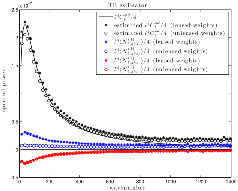
Figure 3: The first order bias term $l^{4}\bigl{\langle}N^{(1)}_{{\bm{l}},\text{\tiny obs}}\bigr{\rangle}/4$ is denoted ‘$\ast$’ for $\tilde{\phi}^{\text{\tiny$X\!Y$}}_{\bm{l}}$ and ‘$\circ$’ for $\hat{\phi}^{\text{\tiny$X\!Y$}}_{\bm{l}}$. The second order bias term $l^{4}\bigl{\langle}N^{(2)}_{{\bm{l}},\text{\tiny obs}}\bigr{\rangle}/4$ is denoted ‘$\ast$’ for $\tilde{\phi}^{\text{\tiny$X\!Y$}}_{\bm{l}}$ and ‘$\circ$’ for $\hat{\phi}^{\text{\tiny$X\!Y$}}_{\bm{l}}$. Finally, the expected value of the spectral density estimates $l^{4}\langle\delta_{0}^{-1}|\hat{\phi}_{\bm{l}}^{\text{\tiny$X\!Y$}}|^{2}-N^{(0)}_{{\bm{l}},\text{\tiny obs}}\rangle/4$ and $l^{4}\langle\delta_{0}^{-1}|\tilde{\phi}_{\bm{l}}^{\text{\tiny$X\!Y$}}|^{2}-N^{(0)}_{{\bm{l}},\text{\tiny obs}}\rangle/4$ are denoted by ‘$\circ$’ and ‘$\ast$’ respectively. See Section VI for details.

IV.1 The bias of $\delta_{0}^{-1}|\hat{\phi}_{\bm{l}}^{\text{\tiny$X\!Y$}}|^{2}-N^{(0)}_{{\bm{l}},\text{\tiny obs}}$

We will derive three main expansions, which decompose the bias: $\bigl{\langle}\delta_{0}^{-1}|\hat{\phi}_{\bm{l}}^{\text{\tiny$X\!Y$}}|^{2}-N^{(0)}_{{\bm{l}},\text{\tiny obs}}\bigr{\rangle}-C_{\bm{l}}^{\phi\phi}$ (and similar definitions for the modified quadratic estimate). These expansions will be denoted as follows

$$\hat{\phi}^{\text{\tiny$X\!Y$}}_{\bm{l}} =\mathscr{L}^{(0)}_{\bm{l}}+\mathscr{L}^{(1)}_{\bm{l}}+\mathscr{L}^{(2)}_{\bm{l}}+\cdots$$ (13)

$$|\hat{\phi}^{\text{\tiny$X\!Y$}}_{\bm{l}}|^{2} =\mathscr{O}^{(0)}_{\bm{l}}\,\,+\mathscr{O}^{(1)}_{\bm{l}}\,\,+\mathscr{O}^{(2)}_{\bm{l}}\,\,+\cdots$$ (14)

$$N^{(0)}_{{\bm{l}},\text{\tiny obs}} =\mathscr{N}^{(0)}_{\bm{l}}+\mathscr{N}^{(1)}_{\bm{l}}+\mathscr{N}^{(2)}_{\bm{l}}+\cdots$$ (15)

where the terms $\mathscr{L}^{(j)}_{\bm{l}}$, $\mathscr{O}^{(j)}_{\bm{l}}$ and $\mathscr{N}^{(j)}_{\bm{l}}$ are each of order $j$ in $\phi$. Expansions (13), (14) and (15) are all obtained by expanding $\tilde{X}_{\bm{k}}$ and $\tilde{Y}_{\bm{k}}$ using (3) then regrouping the terms by the order of $\phi$. This expansion and subsequent re-grouping yields the following analytic expressions for each term:

$$\mathscr{L}^{(j)}_{\bm{l}} \equiv\sum_{p=0}^{j}A^{\text{\tiny$X\!Y$}}_{\bm{l}}\int\frac{d^{2}\bm{k}}{2\pi}g^{\text{\tiny$X\!Y$}}_{\bm{l},\bm{k}\,}\left[\delta^{p}X_{\bm{k}+\bm{l}}\delta^{j-p}Y_{\bm{k}}^{*}\right];$$

$$\mathscr{O}^{(j)}_{\bm{l}} \equiv\sum_{p=0}^{j}\mathscr{L}^{(p)}_{\bm{l}}\mathscr{L}^{(j-p)^{*}}_{\bm{l}};$$

$$\mathscr{N}^{(j)}_{\bm{l}} \equiv\sum_{p=0}^{j}\!\delta_{0}^{\text{\tiny$-2$}}[A^{\text{\tiny$X\!Y$}}_{\bm{l}}]^{2}\!\int\!\!\frac{d^{2}{\bm{k}}}{(2\pi)^{2}}\Bigl{(}g^{\text{\tiny$X\!Y$}}_{\bm{l},{\bm{k}}\,}g^{\text{\tiny$X\!Y$}}_{{\bm{l}},-{\bm{k}}-{\bm{l}}\,}\mathscr{P}^{\text{\tiny$X\!Y$}\!,p}_{{\bm{k}}+{\bm{l}}}\mathscr{P}^{\text{\tiny$X\!Y$}\!,j-p}_{{\bm{k}}}$$

$$\qquad\qquad\qquad\qquad\qquad+|g^{\text{\tiny$X\!Y$}}_{\bm{l},\bm{k}}|^{2}\mathscr{P}^{\text{\tiny$X\!X$},p}_{{\bm{k}}+{\bm{l}}}\mathscr{P}^{\text{\tiny$Y\!Y$},j-p}_{{\bm{k}}}\Bigr{)},$$

where $\mathscr{P}_{\bm{k}}^{\text{\tiny$X\!Y$},j}\equiv\sum_{p=0}^{j}\delta^{p}X_{\bm{k}}\delta^{j-p}Y^{*}_{\bm{k}}$ so that $\tilde{X}_{\bm{k}}\tilde{Y}_{\bm{k}}^{*}=\sum_{p=0}^{\infty}\mathscr{P}^{\text{\tiny$X\!Y$},p}_{\bm{k}}$. Using the fact that $\langle\mathscr{O}^{(2j+1)}_{\bm{l}}\rangle=\langle\mathscr{N}^{(2j+1)}_{\bm{l}}\rangle=0$ one then gets that

$$\bigl{\langle}|\hat{\phi}_{\bm{l}}^{\text{\tiny$X\!Y$}}|^{2}-\delta_{0}N^{(0)}_{{\bm{l}},\text{\tiny obs}}\bigr{\rangle} =\sum_{j=0}^{\infty}\bigl{\langle}\mathscr{O}^{(2j)}_{\bm{l}}-\delta_{0}\mathscr{N}^{(2j)}_{\bm{l}}\bigr{\rangle}.$$ (16)

Now by defining $N_{{\bm{l}},\text{\tiny obs}}^{(j)}$ for $j\geq 1$ as

$$N^{(j)}_{{\bm{l}},\text{\tiny obs}}\equiv\begin{cases}\delta_{0}^{-1}\mathscr{O}^{(2j)}_{\bm{l}}-\mathscr{N}^{(2j)}_{\bm{l}}-C_{\bm{l}}^{\phi\phi}&\text{when $j=1$}\\ \delta_{0}^{-1}\mathscr{O}^{(2j)}_{\bm{l}}-\mathscr{N}^{(2j)}_{\bm{l}}&\text{when $j>1$}\\ \end{cases}$$ (17)

we have that

$$\bigl{\langle}|\hat{\phi}_{\bm{l}}^{\text{\tiny$X\!Y$}}|^{2}\bigr{\rangle} =\delta_{0}\bigl{[}C_{\bm{l}}^{\phi\phi}+\bigl{\langle}N^{(0)}_{{\bm{l}},\text{\tiny obs}}\bigr{\rangle}+\bigl{\langle}N^{(1)}_{{\bm{l}},\text{\tiny obs}}\bigr{\rangle}+\cdots\bigr{]}$$

$$\quad+\bigl{\langle}\mathscr{O}^{(0)}_{\bm{l}}-\delta_{0}\mathscr{N}^{(0)}_{{\bm{l}}}\bigr{\rangle}$$ (18)

where $N^{(j)}_{{\bm{l}},\text{\tiny obs}}$ is of order $\phi^{2j}$. Therefore the order $\phi^{2j}$ term in the bias of $\delta_{0}^{-1}|\hat{\phi}_{\bm{l}}^{\text{\tiny$X\!Y$}}|^{2}-N^{(0)}_{{\bm{l}},\text{\tiny obs}}$ is given by $\bigl{\langle}N^{(j)}_{{\bm{l}},\text{\tiny obs}}\bigr{\rangle}$ for $j\geq 1$.

Remark: Notice that the zero order term can be computed easily

$$\bigl{\langle}\mathscr{O}^{(0)}_{\bm{l}}-\delta_{0}\mathscr{N}^{(0)}_{{\bm{l}}}\bigr{\rangle} =-\frac{[A^{\text{\tiny$X\!Y$}}_{\bm{l}}g^{\text{\tiny$X\!Y$}}_{\bm{l},-{\bm{l}}/2}]^{2}}{(2\pi)^{2}}$$

$$\quad\times\Bigl{[}C^{\text{\tiny$X\!X$}}_{{\bm{l}}/2,\text{\tiny exp}}C^{\text{\tiny$Y\!Y$}}_{{\bm{l}}/2,\text{\tiny exp}}+(C^{\text{\tiny$X\!Y$}}_{{\bm{l}}/2,\text{\tiny exp}})^{2}\Bigr{]}$$

when ${\bm{l}}\neq 0$. Moreover, since this term does not depend on $\phi$ one can simply subtract it out of the estimator when using $\delta_{0}^{-1}|\hat{\phi}_{\bm{l}}^{\text{\tiny$X\!Y$}}|^{2}-N^{(0)}_{{\bm{l}},\text{\tiny obs}}$ for estimation.

IV.2 The difference between $N^{(1)}_{\bm{l}}$ and $\bigl{\langle}N^{(1)}_{{\bm{l}},\text{\tiny obs}}\bigr{\rangle}$

By matching the right hand side of equation (14) with the right hand side of (7) one gets that $\delta_{0}N^{(1)}_{\bm{l}}$ equals $\langle\mathscr{O}^{(2)}_{\bm{l}}\rangle$ minus $\delta_{0}C_{\bm{l}}^{\phi\phi}$ and any disconnected terms. In contrast, $\delta_{0}\bigl{\langle}N^{(1)}_{{\bm{l}},\text{\tiny obs}}\bigr{\rangle}$ equals $\langle\mathscr{O}^{(2)}_{\bm{l}}\rangle$ minus $\delta_{0}C_{\bm{l}}^{\phi\phi}$ and $\langle\delta_{0}\mathscr{N}_{\bm{l}}^{(2)}\rangle$. Therefore the difference between $\delta_{0}N^{(1)}_{\bm{l}}$ and $\delta_{0}\bigl{\langle}N^{(1)}_{{\bm{l}},\text{\tiny obs}}\bigr{\rangle}$ is the difference between $\langle\delta_{0}\mathscr{N}_{\bm{l}}^{(2)}\rangle$ and the disconnected terms in $\langle\mathscr{O}^{(2)}_{\bm{l}}\rangle$. By expanding $\delta_{0}\widetilde{C}^{\text{\tiny$X\!Y$}}_{{\bm{l}},\text{\tiny exp}}=\sum_{p=0}^{\infty}\langle\mathscr{P}^{\text{\tiny$X\!Y$},p}_{\bm{l}}\rangle$ in the definition of $\delta_{0}N^{(0)}_{\bm{l}}$ (which equals all the disconnected terms), and retaining only the order $\phi^{2}$ terms (what remains equals all the disconnected terms in $\langle\mathscr{O}^{(2)}_{\bm{l}}\rangle$) we get

$$\sum_{p=0}^{2}\delta_{0}^{-1}[A^{\text{\tiny$X\!Y$}}_{\bm{l}}]^{2}\int\frac{d^{2}{\bm{k}}}{(2\pi)^{2}}\Bigl{(}g^{\text{\tiny$X\!Y$}}_{\bm{l},{\bm{k}}\,}g^{\text{\tiny$X\!Y$}}_{{\bm{l}},-{\bm{k}}-{\bm{l}}\,}\bigl{\langle}\mathscr{P}^{\text{\tiny$X\!Y$},p}_{{\bm{k}}+{\bm{l}}}\bigr{\rangle}\bigl{\langle}\mathscr{P}^{\text{\tiny$X\!Y$},2-p}_{{\bm{k}}}\bigr{\rangle}$$

$$\qquad\qquad\qquad\qquad+|g^{\text{\tiny$X\!Y$}}_{\bm{l},\bm{k}}|^{2}\bigl{\langle}\mathscr{P}^{\text{\tiny$X\!X$},p}_{{\bm{k}}+{\bm{l}}}\bigr{\rangle}\bigl{\langle}\mathscr{P}^{\text{\tiny$Y\!Y$},2-p}_{{\bm{k}}}\bigr{\rangle}\Bigr{)}.$$ (19)

Therefore the difference between $\delta_{0}N^{(1)}_{\bm{l}}$ and $\delta_{0}\bigl{\langle}N^{(1)}_{{\bm{l}},\text{\tiny obs}}\bigr{\rangle}$ is given by the difference between (19) and $\langle\delta_{0}\mathscr{N}_{\bm{l}}^{(2)}\rangle$ which equals

$$\sum_{p=0}^{2}\delta_{0}^{-1}[A^{\text{\tiny$X\!Y$}}_{\bm{l}}]^{2}\int\frac{d^{2}{\bm{k}}}{(2\pi)^{2}}\Bigl{(}g^{\text{\tiny$X\!Y$}}_{\bm{l},{\bm{k}}\,}g^{\text{\tiny$X\!Y$}}_{{\bm{l}},-{\bm{k}}-{\bm{l}}\,}\left\langle\mathscr{P}^{\text{\tiny$X\!Y$},p}_{{\bm{k}}+{\bm{l}}}\mathscr{P}^{\text{\tiny$X\!Y$},2-p}_{{\bm{k}}}\right\rangle$$

$$\qquad\qquad\qquad\qquad+|g^{\text{\tiny$X\!Y$}}_{\bm{l},\bm{k}}|^{2}\left\langle\mathscr{P}^{\text{\tiny$X\!X$},p}_{{\bm{k}}+{\bm{l}}}\mathscr{P}^{\text{\tiny$Y\!Y$},2-p}_{{\bm{k}}}\right\rangle\Bigr{)}.$$ (20)

For the experimental conditions analyzed in this paper this difference is small.

V Fast Monte Carlo algorithms

In this section we give two simulation based methods for quickly estimating $N_{{\bm{l}}}^{(j)}$ and $\langle N_{{\bm{l}},\text{\tiny obs}}^{(j)}\rangle$ for $j\geq 0$. The first method simply observes that each term $\mathscr{L}^{(j)}_{\bm{l}}$, $\mathscr{O}^{(j)}_{\bm{l}}$ and $\mathscr{N}^{(j)}_{{\bm{l}}}$ have fast Fourier transform characterizations which can be used for simulating $N_{{\bm{l}},\text{\tiny obs}}^{(j)}$ and—by averaging multiple realizations—for estimating $\bigl{\langle}N_{{\bm{l}},\text{\tiny obs}}^{(j)}\bigr{\rangle}$. This algorithm also extends to $N^{(j)}_{{\bm{l}}}$ by replacing the expansion of $N_{{\bm{l}},\text{\tiny obs}}^{(0)}$ in (15) with the corresponding expansion for $N_{{\bm{l}}}^{(0)}$. The second method is exclusive to $N^{(1)}_{{\bm{l}}}$ and uses correlated and uncorrelated CMB fields to mimic the appropriate Wick contractions for the connected terms in (8).

V.1 FFT algorithms for $N^{(j)}_{{\bm{l}},\text{\tiny obs}}$ and $N^{(j)}_{{\bm{l}}}$

The fast simulation techniques presented in this section depend on the fact that the transforms which characterize $\hat{\phi}_{\bm{l}}^{\text{\tiny$X\!Y$}}$ and $\tilde{\phi}_{\bm{l}}^{\text{\tiny$X\!Y$}}$ can be derived as Fourier transforms of point-wise products of gradients in pixel space. This was first utilized in Hu (2001) and Hu and Okamoto (2002) for the flat sky quadratic estimators. In the appendix, we present these transforms along with some additional FFT transforms which allow fast simulation of the fields $\mathscr{L}^{(j)}_{\bm{l}}$, $\mathscr{O}^{(j)}_{\bm{l}}$ and $\mathscr{N}^{(j)}_{{\bm{l}}}$. This is the basis of the algorithm which then uses equation (17) to simulate $N^{(j)}_{{\bm{l}},\text{\tiny obs}}$.

For $\mathscr{L}^{(j)}_{\bm{l}}$ and $\mathscr{O}^{(j)}_{\bm{l}}$ first notice that each term $\delta^{j}X_{\bm{l}}$ can be easily simulated in the pixel domain since $\delta^{j}X(\bm{x})$ is the point-wise product of derivatives of $X(\bm{x})$ and $\phi(\bm{x})$. Moreover the quadratic estimate applied to these terms, resulting in $A^{\text{\tiny$X\!Y$}}_{\bm{l}}\int\frac{d^{2}\bm{k}}{2\pi}g^{\text{\tiny$X\!Y$}}_{\bm{l},\bm{k}\,}\left[\delta^{p}X_{\bm{k}+\bm{l}}\delta^{j-p}Y_{\bm{k}}^{*}\right]$, is also easily computed by direct application of the formulas presented in the Appendix. Now summing over $p\in\{0,\ldots,j\}$ gives fast simulation of $\mathscr{L}^{(j)}_{\bm{l}}$ which, in turn, gives $\mathscr{O}^{(j)}_{\bm{l}}$ by taking quadratic combinations of $\mathscr{L}^{(0)}_{\bm{l}}\!,\ldots,\mathscr{L}^{(j)}_{\bm{l}}$. Finally, to simulate $\mathscr{N}^{(j)}_{\bm{l}}$ start by noticing that each term $\mathscr{P}_{\bm{k}}^{\text{\tiny$X\!Y$},j}\equiv\sum_{p=0}^{j}\delta^{p}X_{\bm{k}}\delta^{j-p}Y^{*}_{\bm{k}}$ simulates easily from $\delta^{p}X_{\bm{k}}$ and $\delta^{j-p}Y_{\bm{k}}^{*}$. Then to recover $\mathscr{N}^{(j)}_{\bm{l}}$ one uses the FFT transformations presented in the appendix for quick simulations of $[A^{\text{\tiny$X\!Y$}}_{\bm{l}}]^{2}\!\int\!\!\frac{d^{2}{\bm{k}}}{(2\pi)^{2}}g^{\text{\tiny$X\!Y$}}_{\bm{l},{\bm{k}}\,}g^{\text{\tiny$X\!Y$}}_{{\bm{l}},-{\bm{k}}-{\bm{l}}\,}\mathscr{P}^{\text{\tiny$X\!Y$}\!,p}_{{\bm{k}}+{\bm{l}}}\mathscr{P}^{\text{\tiny$X\!Y$}\!,j-p}_{{\bm{k}}}$ and $[A^{\text{\tiny$X\!Y$}}_{\bm{l}}]^{2}\!\int\!\!\frac{d^{2}{\bm{k}}}{(2\pi)^{2}}|g^{\text{\tiny$X\!Y$}}_{\bm{l},\bm{k}}|^{2}\mathscr{P}^{\text{\tiny$X\!X$},p}_{{\bm{k}}+{\bm{l}}}\mathscr{P}^{\text{\tiny$Y\!Y$},2-p}_{{\bm{k}}}$.

Monte Carlo averaging $n$ independent simulations of $N_{{\bm{l}},\text{\tiny obs}}^{(j)}$ will yield estimates of $\bigl{\langle}N_{{\bm{l}},\text{\tiny obs}}^{(j)}\bigr{\rangle}$ with error bars that can be approximated by $s_{\bm{l}}/\sqrt{n}$ where $s_{\bm{l}}$ denotes the standard deviation of the samples at each frequency ${\bm{l}}$. In addition, when the noise and beam structure are isotropic one can reduce the error bars by radially averaging each simulation of $N_{{\bm{l}},\text{\tiny obs}}^{(j)}$. These error bars can then be used for re-fitting algorithms where $C_{\bm{l}}^{\phi\phi}$ is iteratively fit to $\delta_{0}^{-1}|\hat{\phi}_{\bm{l}}^{\text{\tiny$X\!Y$}}|^{2}-N^{(0)}_{{\bm{l}},\text{\tiny obs}}-\mu_{\bm{l}}$ where $\mu_{\bm{l}}$ is an approximate bias correction based on the estimates of the higher order bias correction terms $\bigl{\langle}N_{{\bm{l}},\text{\tiny obs}}^{(j)}\bigr{\rangle}$. Notice that for fast re-fitting algorithms, it maybe be advantageous initially to tolerate relatively large the Monte Carlo error bars, then iteratively increase the number of Monte Carlo samples at each re-fit.

We finally mention that the above simulation methods which are used to estimate $\bigl{\langle}N_{{\bm{l}},\text{\tiny obs}}^{(j)}\bigr{\rangle}$ can also be used to estimate $N^{(j)}_{{\bm{l}}}$. The only change is to replace each term $\mathscr{P}^{\text{\tiny$X\!Y$},p}_{{\bm{k}}+{\bm{l}}}$, $\mathscr{P}^{\text{\tiny$X\!Y$},2j-p}_{{\bm{k}}}$, $\mathscr{P}^{\text{\tiny$X\!X$},p}_{{\bm{k}}+{\bm{l}}}$ and $\mathscr{P}^{\text{\tiny$X\!X$},2j-p}_{{\bm{k}}}$ in the definition of $\mathscr{N}^{(2j)}_{\bm{l}}$ with their respective expected values: $\bigl{\langle}\mathscr{P}^{\text{\tiny$X\!Y$},p}_{{\bm{k}}+{\bm{l}}}\bigr{\rangle}$, $\bigl{\langle}\mathscr{P}^{\text{\tiny$X\!Y$},2j-p}_{{\bm{k}}}\bigr{\rangle}$, $\bigl{\langle}\mathscr{P}^{\text{\tiny$X\!X$},p}_{{\bm{k}}+{\bm{l}}}\bigr{\rangle}$ and $\bigl{\langle}\mathscr{P}^{\text{\tiny$X\!X$},2j-p}_{{\bm{k}}}\bigr{\rangle}$.

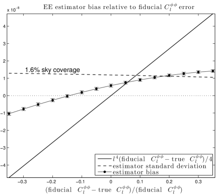
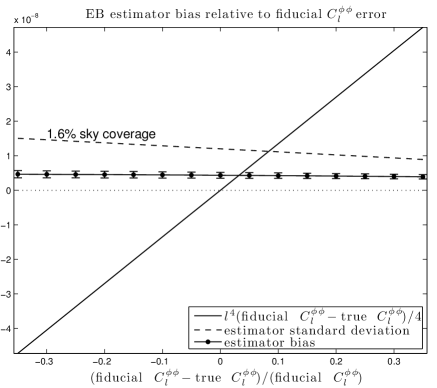
Figure 4: Spectral estimation bias averaged over the multiple bin $l\in[10,200]$ as a function of fiducial uncertainty. See Section VI for details.

V.2 Coupling lensing fields for $N^{(1)}_{{\bm{l}}}$

A second algorithm, for Monte Carlo estimation of $N^{(1)}_{{\bm{l}}}$, is to use correlated and uncorrelated CMB fields to mimic the Wick contraction structure appearing in the definition of $N^{(1)}_{{\bm{l}}}$. The algorithm is easiest to illustrate with the EB quadratic estimator since the definition of $N^{(1)}_{{\bm{l}}}$ only involves a small number of connected terms in (8) (when assuming a zero B mode in the unlensed CMB polarization field). The algorithm is derived by first noticing that the sum of the connected terms of order $\phi^{2}$ in $\langle\hat{\phi}^{\text{\tiny$X\!Y$}}_{\bm{l}}\hat{\phi}^{\text{\tiny$X\!Y$}^{*}}_{{\bm{l}}^{\prime}}\rangle$ is given by

$$\delta_{{\bm{l}}-{\bm{l}}^{\prime}}\bigl{[}N_{\bm{l}}^{(1)}+C_{\bm{l}}^{\phi\phi}\bigr{]}= A^{\text{\tiny$X\!Y$}}_{\bm{l}}A^{\text{\tiny$X\!Y$}}_{{\bm{l}}^{\prime}}\int\frac{d^{2}{\bm{k}}}{2\pi}\int\frac{d^{2}{\bm{k}}^{\prime}}{2\pi}g^{\text{\tiny$X\!Y$}}_{\bm{l},{\bm{k}}\,}g^{\text{\tiny$X\!Y$}}_{\bm{l}^{\prime},{\bm{k}}^{\prime}\,}$$

$$\times\Bigl{[}\bigl{\langle}\mathchoice{\vbox{\hbox to0.0pt{\kern 0.0pt\kern 11.38223pt\hbox{\vrule width=0.50003pt,height=0.0pt,depth=4.30554pt\vrule width=19.61455pt,height=0.0pt,depth=0.50003pt\vrule width=0.50003pt,height=0.0pt,depth=4.30554pt}\hss}\vskip 2.15277pt\vskip 8.74889pt}}{\vbox{\hbox to0.0pt{\kern 0.0pt\kern 11.38223pt\hbox{\vrule width=0.50003pt,height=0.0pt,depth=4.30554pt\vrule width=19.61455pt,height=0.0pt,depth=0.50003pt\vrule width=0.50003pt,height=0.0pt,depth=4.30554pt}\hss}\vskip 2.15277pt\vskip 8.74889pt}}{\vbox{\hbox to0.0pt{\kern 0.0pt\kern 7.80348pt\hbox{\vrule width=0.50003pt,height=0.0pt,depth=4.30554pt\vrule width=13.3561pt,height=0.0pt,depth=0.50003pt\vrule width=0.50003pt,height=0.0pt,depth=4.30554pt}\hss}\vskip 2.15277pt\vskip 6.14998pt}}{\vbox{\hbox to0.0pt{\kern 0.0pt\kern 6.5632pt\hbox{\vrule width=0.50003pt,height=0.0pt,depth=4.30554pt\vrule width=10.86269pt,height=0.0pt,depth=0.50003pt\vrule width=0.50003pt,height=0.0pt,depth=4.30554pt}\hss}\vskip 2.15277pt\vskip 4.7611pt}}\mathchoice{\vbox{\hbox to0.0pt{\kern 39.22911pt\kern 8.16806pt\hbox{\vrule width=0.50003pt,height=0.0pt,depth=4.30554pt\vrule width=16.9862pt,height=0.0pt,depth=0.50003pt\vrule width=0.50003pt,height=0.0pt,depth=4.30554pt}\hss}\vskip 2.15277pt\vskip 8.74889pt}}{\vbox{\hbox to0.0pt{\kern 39.22911pt\kern 8.16806pt\hbox{\vrule width=0.50003pt,height=0.0pt,depth=4.30554pt\vrule width=16.9862pt,height=0.0pt,depth=0.50003pt\vrule width=0.50003pt,height=0.0pt,depth=4.30554pt}\hss}\vskip 2.15277pt\vskip 8.74889pt}}{\vbox{\hbox to0.0pt{\kern 26.71219pt\kern 5.50764pt\hbox{\vrule width=0.50003pt,height=0.0pt,depth=4.30554pt\vrule width=11.60442pt,height=0.0pt,depth=0.50003pt\vrule width=0.50003pt,height=0.0pt,depth=4.30554pt}\hss}\vskip 2.15277pt\vskip 6.14998pt}}{\vbox{\hbox to0.0pt{\kern 21.72539pt\kern 4.26736pt\hbox{\vrule width=0.50003pt,height=0.0pt,depth=4.30554pt\vrule width=9.11101pt,height=0.0pt,depth=0.50003pt\vrule width=0.50003pt,height=0.0pt,depth=4.30554pt}\hss}\vskip 2.15277pt\vskip 4.7611pt}}\mathchoice{\lower 2.15277pt\vbox{\hbox to0.0pt{\kern 22.76448pt\kern 8.23232pt\hbox{\vrule width=0.50003pt,height=0.0pt,depth=4.30554pt\lower 3.80551pt\hbox{\vrule width=33.38658pt,height=0.0pt,depth=0.50003pt}\vrule width=0.50003pt,height=0.0pt,depth=4.30554pt}\hss}}}{\lower 2.15277pt\vbox{\hbox to0.0pt{\kern 22.76448pt\kern 8.23232pt\hbox{\vrule width=0.50003pt,height=0.0pt,depth=4.30554pt\lower 3.80551pt\hbox{\vrule width=33.38658pt,height=0.0pt,depth=0.50003pt}\vrule width=0.50003pt,height=0.0pt,depth=4.30554pt}\hss}}}{\lower 2.15277pt\vbox{\hbox to0.0pt{\kern 15.60696pt\kern 5.55261pt\hbox{\vrule width=0.50003pt,height=0.0pt,depth=4.30554pt\lower 3.80551pt\hbox{\vrule width=22.66467pt,height=0.0pt,depth=0.50003pt}\vrule width=0.50003pt,height=0.0pt,depth=4.30554pt}\hss}}}{\lower 2.15277pt\vbox{\hbox to0.0pt{\kern 13.1264pt\kern 4.29948pt\hbox{\vrule width=0.50003pt,height=0.0pt,depth=4.30554pt\lower 3.80551pt\hbox{\vrule width=17.67787pt,height=0.0pt,depth=0.50003pt}\vrule width=0.50003pt,height=0.0pt,depth=4.30554pt}\hss}}}{\delta^{0}\!E_{{\bm{k}}+{\bm{l}}}}{\delta^{1}\!B^{*}_{{\bm{k}}}}{\delta^{0}\!E^{*}_{{\bm{k}}^{\prime}+{\bm{l}}^{\prime}}}{\delta^{1}\!B_{{\bm{k}}^{\prime}}}\bigr{\rangle}$$

$$\qquad+\bigl{\langle}\mathchoice{\vbox{\hbox to0.0pt{\kern 0.0pt\kern 11.38223pt\hbox{\vrule width=0.50003pt,height=0.0pt,depth=8.61108pt\vrule width=53.00114pt,height=0.0pt,depth=0.50003pt\vrule width=0.50003pt,height=0.0pt,depth=8.61108pt}\hss}\vskip 2.15277pt\vskip 8.74889pt}}{\vbox{\hbox to0.0pt{\kern 0.0pt\kern 11.38223pt\hbox{\vrule width=0.50003pt,height=0.0pt,depth=8.61108pt\vrule width=53.00114pt,height=0.0pt,depth=0.50003pt\vrule width=0.50003pt,height=0.0pt,depth=8.61108pt}\hss}\vskip 2.15277pt\vskip 8.74889pt}}{\vbox{\hbox to0.0pt{\kern 0.0pt\kern 7.80348pt\hbox{\vrule width=0.50003pt,height=0.0pt,depth=8.61108pt\vrule width=36.02077pt,height=0.0pt,depth=0.50003pt\vrule width=0.50003pt,height=0.0pt,depth=8.61108pt}\hss}\vskip 2.15277pt\vskip 6.14998pt}}{\vbox{\hbox to0.0pt{\kern 0.0pt\kern 6.5632pt\hbox{\vrule width=0.50003pt,height=0.0pt,depth=8.61108pt\vrule width=28.54056pt,height=0.0pt,depth=0.50003pt\vrule width=0.50003pt,height=0.0pt,depth=8.61108pt}\hss}\vskip 2.15277pt\vskip 4.7611pt}}\mathchoice{\vbox{\hbox to0.0pt{\kern 22.76448pt\kern 8.23232pt\hbox{\vrule width=0.50003pt,height=0.0pt,depth=4.30554pt\vrule width=16.40038pt,height=0.0pt,depth=0.50003pt\vrule width=0.50003pt,height=0.0pt,depth=4.30554pt}\hss}\vskip 2.15277pt\vskip 8.74889pt}}{\vbox{\hbox to0.0pt{\kern 22.76448pt\kern 8.23232pt\hbox{\vrule width=0.50003pt,height=0.0pt,depth=4.30554pt\vrule width=16.40038pt,height=0.0pt,depth=0.50003pt\vrule width=0.50003pt,height=0.0pt,depth=4.30554pt}\hss}\vskip 2.15277pt\vskip 8.74889pt}}{\vbox{\hbox to0.0pt{\kern 15.60696pt\kern 5.55261pt\hbox{\vrule width=0.50003pt,height=0.0pt,depth=4.30554pt\vrule width=11.06026pt,height=0.0pt,depth=0.50003pt\vrule width=0.50003pt,height=0.0pt,depth=4.30554pt}\hss}\vskip 2.15277pt\vskip 6.14998pt}}{\vbox{\hbox to0.0pt{\kern 13.1264pt\kern 4.29948pt\hbox{\vrule width=0.50003pt,height=0.0pt,depth=4.30554pt\vrule width=8.56685pt,height=0.0pt,depth=0.50003pt\vrule width=0.50003pt,height=0.0pt,depth=4.30554pt}\hss}\vskip 2.15277pt\vskip 4.7611pt}}\mathchoice{\lower 2.15277pt\vbox{\hbox to0.0pt{\kern 22.76448pt\kern 8.23232pt\hbox{\vrule width=0.50003pt,height=0.0pt,depth=4.30554pt\lower 3.80551pt\hbox{\vrule width=33.38658pt,height=0.0pt,depth=0.50003pt}\vrule width=0.50003pt,height=0.0pt,depth=4.30554pt}\hss}}}{\lower 2.15277pt\vbox{\hbox to0.0pt{\kern 22.76448pt\kern 8.23232pt\hbox{\vrule width=0.50003pt,height=0.0pt,depth=4.30554pt\lower 3.80551pt\hbox{\vrule width=33.38658pt,height=0.0pt,depth=0.50003pt}\vrule width=0.50003pt,height=0.0pt,depth=4.30554pt}\hss}}}{\lower 2.15277pt\vbox{\hbox to0.0pt{\kern 15.60696pt\kern 5.55261pt\hbox{\vrule width=0.50003pt,height=0.0pt,depth=4.30554pt\lower 3.80551pt\hbox{\vrule width=22.66467pt,height=0.0pt,depth=0.50003pt}\vrule width=0.50003pt,height=0.0pt,depth=4.30554pt}\hss}}}{\lower 2.15277pt\vbox{\hbox to0.0pt{\kern 13.1264pt\kern 4.29948pt\hbox{\vrule width=0.50003pt,height=0.0pt,depth=4.30554pt\lower 3.80551pt\hbox{\vrule width=17.67787pt,height=0.0pt,depth=0.50003pt}\vrule width=0.50003pt,height=0.0pt,depth=4.30554pt}\hss}}}{\delta^{0}\!E_{{\bm{k}}+{\bm{l}}}}{\delta^{1}\!B^{*}_{{\bm{k}}}}{\delta^{0}\!E^{*}_{{\bm{k}}^{\prime}+{\bm{l}}^{\prime}}}{\delta^{1}\!B_{{\bm{k}}^{\prime}}}\bigr{\rangle}\Bigr{]}$$

These two Wick contraction terms have a Monte Carlo characterization as follows. Let $(Q_{\bm{l}}^{\phantom{\prime}},U_{\bm{l}}^{\phantom{\prime}})$ and $(Q_{\bm{l}}^{\prime},U_{\bm{l}}^{\prime})$ denote two independent realizations of the CMB polarization. Now let $\hat{\phi}^{\text{\tiny$E\!B$}}_{{\bm{l}},1}$ and $\hat{\phi}^{\text{\tiny$E\!B$}}_{{\bm{l}},2}$ denote the EB quadratic estimator applied to the pairs $(E_{\bm{l}}^{\phantom{\prime}},\delta^{1}\!B_{\bm{l}}^{\phantom{\prime}})$ and $(E^{\prime}_{\bm{l}},\delta^{1}\!B_{\bm{l}}^{\prime})$, respectively, where $\delta^{1}\!B^{\phantom{\prime}}$ and $\delta^{1}\!B^{\prime}$ use the same lensing potential $\phi$ so that

$$\delta^{1}\!B_{\bm{l}} \equiv\sin(2\varphi_{\bm{l}})\delta^{1}Q_{\bm{l}}-\cos(2\varphi_{\bm{l}})\delta^{1}U_{\bm{l}}$$

$$\delta^{1}\!B^{\prime}_{\bm{l}} \equiv\sin(2\varphi_{\bm{l}})\delta^{1}Q^{\prime}_{\bm{l}}-\cos(2\varphi_{\bm{l}})\delta^{1}U^{\prime}_{\bm{l}}$$

where $\delta^{1}\!Q^{\phantom{\prime}}(\bm{x})\equiv\nabla^{a}Q(\bm{x})\nabla_{a}\phi(\bm{x})$ and $\delta^{1}\!Q^{\prime}(\bm{x})\equiv\nabla^{a}Q^{\prime}(\bm{x})\nabla_{a}\phi(\bm{x})$ (similar definitions for $\delta^{1}\!U^{\phantom{\prime}}(\bm{x})$ and $\delta^{1}\!U^{\prime}(\bm{x})$). Notice the independence structure of the simulated fields–that $E$ and $B$ are independent of $E^{\prime}$ and $B^{\prime}$—implies

$$\bigl{\langle}\hat{\phi}^{\text{\tiny$E\!B$}}_{{\bm{l}},1}\hat{\phi}^{\text{\tiny$E\!B$}^{*}}_{{\bm{l}}^{\prime},2}\bigr{\rangle}=A^{\text{\tiny$X\!Y$}}_{\bm{l}}A^{\text{\tiny$X\!Y$}}_{{\bm{l}}^{\prime}} \int\frac{d^{2}{\bm{k}}}{2\pi}\int\frac{d^{2}{\bm{k}}^{\prime}}{2\pi}g^{\text{\tiny$X\!Y$}}_{\bm{l},{\bm{k}}\,}g^{\text{\tiny$X\!Y$}}_{\bm{l}^{\prime},{\bm{k}}^{\prime}\,}$$

$$\times\bigl{\langle}\mathchoice{\vbox{\hbox to0.0pt{\kern 0.0pt\kern 11.38223pt\hbox{\vrule width=0.50003pt,height=0.0pt,depth=4.30554pt\vrule width=19.61455pt,height=0.0pt,depth=0.50003pt\vrule width=0.50003pt,height=0.0pt,depth=4.30554pt}\hss}\vskip 2.15277pt\vskip 8.74889pt}}{\vbox{\hbox to0.0pt{\kern 0.0pt\kern 11.38223pt\hbox{\vrule width=0.50003pt,height=0.0pt,depth=4.30554pt\vrule width=19.61455pt,height=0.0pt,depth=0.50003pt\vrule width=0.50003pt,height=0.0pt,depth=4.30554pt}\hss}\vskip 2.15277pt\vskip 8.74889pt}}{\vbox{\hbox to0.0pt{\kern 0.0pt\kern 7.80348pt\hbox{\vrule width=0.50003pt,height=0.0pt,depth=4.30554pt\vrule width=13.3561pt,height=0.0pt,depth=0.50003pt\vrule width=0.50003pt,height=0.0pt,depth=4.30554pt}\hss}\vskip 2.15277pt\vskip 6.14998pt}}{\vbox{\hbox to0.0pt{\kern 0.0pt\kern 6.5632pt\hbox{\vrule width=0.50003pt,height=0.0pt,depth=4.30554pt\vrule width=10.86269pt,height=0.0pt,depth=0.50003pt\vrule width=0.50003pt,height=0.0pt,depth=4.30554pt}\hss}\vskip 2.15277pt\vskip 4.7611pt}}\mathchoice{\vbox{\hbox to0.0pt{\kern 39.22911pt\kern 8.16806pt\hbox{\vrule width=0.50003pt,height=0.0pt,depth=4.30554pt\vrule width=16.9862pt,height=0.0pt,depth=0.50003pt\vrule width=0.50003pt,height=0.0pt,depth=4.30554pt}\hss}\vskip 2.15277pt\vskip 8.74889pt}}{\vbox{\hbox to0.0pt{\kern 39.22911pt\kern 8.16806pt\hbox{\vrule width=0.50003pt,height=0.0pt,depth=4.30554pt\vrule width=16.9862pt,height=0.0pt,depth=0.50003pt\vrule width=0.50003pt,height=0.0pt,depth=4.30554pt}\hss}\vskip 2.15277pt\vskip 8.74889pt}}{\vbox{\hbox to0.0pt{\kern 26.71219pt\kern 5.50764pt\hbox{\vrule width=0.50003pt,height=0.0pt,depth=4.30554pt\vrule width=11.60442pt,height=0.0pt,depth=0.50003pt\vrule width=0.50003pt,height=0.0pt,depth=4.30554pt}\hss}\vskip 2.15277pt\vskip 6.14998pt}}{\vbox{\hbox to0.0pt{\kern 21.72539pt\kern 4.26736pt\hbox{\vrule width=0.50003pt,height=0.0pt,depth=4.30554pt\vrule width=9.11101pt,height=0.0pt,depth=0.50003pt\vrule width=0.50003pt,height=0.0pt,depth=4.30554pt}\hss}\vskip 2.15277pt\vskip 4.7611pt}}\mathchoice{\lower 2.15277pt\vbox{\hbox to0.0pt{\kern 22.76448pt\kern 8.23232pt\hbox{\vrule width=0.50003pt,height=0.0pt,depth=4.30554pt\lower 3.80551pt\hbox{\vrule width=33.38658pt,height=0.0pt,depth=0.50003pt}\vrule width=0.50003pt,height=0.0pt,depth=4.30554pt}\hss}}}{\lower 2.15277pt\vbox{\hbox to0.0pt{\kern 22.76448pt\kern 8.23232pt\hbox{\vrule width=0.50003pt,height=0.0pt,depth=4.30554pt\lower 3.80551pt\hbox{\vrule width=33.38658pt,height=0.0pt,depth=0.50003pt}\vrule width=0.50003pt,height=0.0pt,depth=4.30554pt}\hss}}}{\lower 2.15277pt\vbox{\hbox to0.0pt{\kern 15.60696pt\kern 5.55261pt\hbox{\vrule width=0.50003pt,height=0.0pt,depth=4.30554pt\lower 3.80551pt\hbox{\vrule width=22.66467pt,height=0.0pt,depth=0.50003pt}\vrule width=0.50003pt,height=0.0pt,depth=4.30554pt}\hss}}}{\lower 2.15277pt\vbox{\hbox to0.0pt{\kern 13.1264pt\kern 4.29948pt\hbox{\vrule width=0.50003pt,height=0.0pt,depth=4.30554pt\lower 3.80551pt\hbox{\vrule width=17.67787pt,height=0.0pt,depth=0.50003pt}\vrule width=0.50003pt,height=0.0pt,depth=4.30554pt}\hss}}}{\delta^{0}\!E_{{\bm{k}}+{\bm{l}}}}{\delta^{1}\!B^{*}_{{\bm{k}}}}{\delta^{0}\!E^{*}_{{\bm{k}}^{\prime}+{\bm{l}}^{\prime}}}{\delta^{1}\!B_{{\bm{k}}^{\prime}}}\bigr{\rangle}.$$

Similarly let $\hat{\phi}^{\text{\tiny$E\!B$}}_{{\bm{l}},3}$ and $\hat{\phi}^{\text{\tiny$E\!B$}}_{{\bm{l}},4}$ denote the EB quadratic estimator applied to the pairs $(E_{\bm{l}}^{\prime},\delta^{1}\!B_{\bm{l}}^{\phantom{\prime}})$ and $(E_{\bm{l}}^{\phantom{\prime}},\delta^{1}\!B_{\bm{l}}^{\prime})$ respectively (again using the same lensing potential $\phi$). Then

$$\bigl{\langle}\hat{\phi}^{\text{\tiny$E\!B$}}_{{\bm{l}},3}\hat{\phi}^{\text{\tiny$E\!B$}^{*}}_{{\bm{l}}^{\prime},4}\bigr{\rangle}=A^{\text{\tiny$X\!Y$}}_{\bm{l}}A^{\text{\tiny$X\!Y$}}_{{\bm{l}}^{\prime}} \int\frac{d^{2}{\bm{k}}}{2\pi}\int\frac{d^{2}{\bm{k}}^{\prime}}{2\pi}g^{\text{\tiny$X\!Y$}}_{\bm{l},{\bm{k}}\,}g^{\text{\tiny$X\!Y$}}_{\bm{l}^{\prime},{\bm{k}}^{\prime}\,}$$

$$\times\bigl{\langle}\mathchoice{\vbox{\hbox to0.0pt{\kern 0.0pt\kern 11.38223pt\hbox{\vrule width=0.50003pt,height=0.0pt,depth=8.61108pt\vrule width=53.00114pt,height=0.0pt,depth=0.50003pt\vrule width=0.50003pt,height=0.0pt,depth=8.61108pt}\hss}\vskip 2.15277pt\vskip 8.74889pt}}{\vbox{\hbox to0.0pt{\kern 0.0pt\kern 11.38223pt\hbox{\vrule width=0.50003pt,height=0.0pt,depth=8.61108pt\vrule width=53.00114pt,height=0.0pt,depth=0.50003pt\vrule width=0.50003pt,height=0.0pt,depth=8.61108pt}\hss}\vskip 2.15277pt\vskip 8.74889pt}}{\vbox{\hbox to0.0pt{\kern 0.0pt\kern 7.80348pt\hbox{\vrule width=0.50003pt,height=0.0pt,depth=8.61108pt\vrule width=36.02077pt,height=0.0pt,depth=0.50003pt\vrule width=0.50003pt,height=0.0pt,depth=8.61108pt}\hss}\vskip 2.15277pt\vskip 6.14998pt}}{\vbox{\hbox to0.0pt{\kern 0.0pt\kern 6.5632pt\hbox{\vrule width=0.50003pt,height=0.0pt,depth=8.61108pt\vrule width=28.54056pt,height=0.0pt,depth=0.50003pt\vrule width=0.50003pt,height=0.0pt,depth=8.61108pt}\hss}\vskip 2.15277pt\vskip 4.7611pt}}\mathchoice{\vbox{\hbox to0.0pt{\kern 22.76448pt\kern 8.23232pt\hbox{\vrule width=0.50003pt,height=0.0pt,depth=4.30554pt\vrule width=16.40038pt,height=0.0pt,depth=0.50003pt\vrule width=0.50003pt,height=0.0pt,depth=4.30554pt}\hss}\vskip 2.15277pt\vskip 8.74889pt}}{\vbox{\hbox to0.0pt{\kern 22.76448pt\kern 8.23232pt\hbox{\vrule width=0.50003pt,height=0.0pt,depth=4.30554pt\vrule width=16.40038pt,height=0.0pt,depth=0.50003pt\vrule width=0.50003pt,height=0.0pt,depth=4.30554pt}\hss}\vskip 2.15277pt\vskip 8.74889pt}}{\vbox{\hbox to0.0pt{\kern 15.60696pt\kern 5.55261pt\hbox{\vrule width=0.50003pt,height=0.0pt,depth=4.30554pt\vrule width=11.06026pt,height=0.0pt,depth=0.50003pt\vrule width=0.50003pt,height=0.0pt,depth=4.30554pt}\hss}\vskip 2.15277pt\vskip 6.14998pt}}{\vbox{\hbox to0.0pt{\kern 13.1264pt\kern 4.29948pt\hbox{\vrule width=0.50003pt,height=0.0pt,depth=4.30554pt\vrule width=8.56685pt,height=0.0pt,depth=0.50003pt\vrule width=0.50003pt,height=0.0pt,depth=4.30554pt}\hss}\vskip 2.15277pt\vskip 4.7611pt}}\mathchoice{\lower 2.15277pt\vbox{\hbox to0.0pt{\kern 22.76448pt\kern 8.23232pt\hbox{\vrule width=0.50003pt,height=0.0pt,depth=4.30554pt\lower 3.80551pt\hbox{\vrule width=33.38658pt,height=0.0pt,depth=0.50003pt}\vrule width=0.50003pt,height=0.0pt,depth=4.30554pt}\hss}}}{\lower 2.15277pt\vbox{\hbox to0.0pt{\kern 22.76448pt\kern 8.23232pt\hbox{\vrule width=0.50003pt,height=0.0pt,depth=4.30554pt\lower 3.80551pt\hbox{\vrule width=33.38658pt,height=0.0pt,depth=0.50003pt}\vrule width=0.50003pt,height=0.0pt,depth=4.30554pt}\hss}}}{\lower 2.15277pt\vbox{\hbox to0.0pt{\kern 15.60696pt\kern 5.55261pt\hbox{\vrule width=0.50003pt,height=0.0pt,depth=4.30554pt\lower 3.80551pt\hbox{\vrule width=22.66467pt,height=0.0pt,depth=0.50003pt}\vrule width=0.50003pt,height=0.0pt,depth=4.30554pt}\hss}}}{\lower 2.15277pt\vbox{\hbox to0.0pt{\kern 13.1264pt\kern 4.29948pt\hbox{\vrule width=0.50003pt,height=0.0pt,depth=4.30554pt\lower 3.80551pt\hbox{\vrule width=17.67787pt,height=0.0pt,depth=0.50003pt}\vrule width=0.50003pt,height=0.0pt,depth=4.30554pt}\hss}}}{\delta^{0}\!E_{{\bm{k}}+{\bm{l}}}}{\delta^{1}\!B^{*}_{{\bm{k}}}}{\delta^{0}\!E^{*}_{{\bm{k}}^{\prime}+{\bm{l}}^{\prime}}}{\delta^{1}\!B_{{\bm{k}}^{\prime}}}\bigr{\rangle}.$$

This leads to the following Monte Carlo averaging characterization of $N^{(1)}_{\bm{l}}$

$$N_{\bm{l}}^{(1)}=\delta_{0}^{-1}\bigl{\langle}\hat{\phi}^{\text{\tiny$E\!B$}}_{{\bm{l}},1}\hat{\phi}^{\text{\tiny$E\!B$}^{*}}_{{\bm{l}},2}+\hat{\phi}^{\text{\tiny$E\!B$}}_{{\bm{l}},3}\hat{\phi}^{\text{\tiny$E\!B$}^{*}}_{{\bm{l}},4}\bigr{\rangle}-C_{\bm{l}}^{\phi\phi}.$$ (21)

The above formula also holds for the lensed quadratic estimator $\tilde{\phi}^{\text{\tiny$E\!B$}}_{{\bm{l}}}$ as well. It is easy to see that this method can be extended to all other polarization quadratic estimators, but with decidedly more connected terms.

Notice that there is an additional simplification when using the quadratic estimator, $\hat{\phi}^{\text{\tiny$E\!B$}}_{\bm{l}}$, without lensed weights. In particular, $\delta_{0}^{-1}\bigl{\langle}\hat{\phi}^{\text{\tiny$E\!B$}}_{{\bm{l}},3}\hat{\phi}^{\text{\tiny$E\!B$}^{*}}_{{\bm{l}},4}\bigr{\rangle}=C_{\bm{l}}^{\phi\phi}$ so that equation (21) simplifies to $N_{\bm{l}}^{(1)}=\delta_{0}^{-1}\bigl{\langle}\hat{\phi}^{\text{\tiny$E\!B$}}_{{\bm{l}},1}\hat{\phi}^{\text{\tiny$E\!B$}^{*}}_{{\bm{l}},2}\bigr{\rangle}$. However, this simplification does not hold for $\tilde{\phi}^{\text{\tiny$E\!B$}}_{\bm{l}}$ since the bias factor $B_{\bm{l}}^{\text{\tiny$E\!B$}}$, defined in Section II.1, implies $\delta_{0}^{-1}\bigl{\langle}\tilde{\phi}^{\text{\tiny$E\!B$}}_{{\bm{l}},3}\tilde{\phi}^{\text{\tiny$E\!B$}^{*}}_{{\bm{l}},4}\bigr{\rangle}=[B_{\bm{l}}^{\text{\tiny$E\!B$}}]^{2}C_{\bm{l}}^{\phi\phi}\neq C_{\bm{l}}^{\phi\phi}$.

One advantage of using this coupling technique is that the simulation of the $\delta^{0}X$ and $\delta^{0}Y$ can be done without including the additive experimental noise. To see why, notice that any CMB Wick contraction connecting $\delta^{0}X$ and $\delta^{0}Y$ (which depends on the additive experimental noise) must have bottom contraction symbols connect $\delta^{1}X$ and $\delta^{1}Y$. This must yield a disconnected term which does not contribute to $N^{(1)}_{\bm{l}}$.

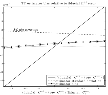
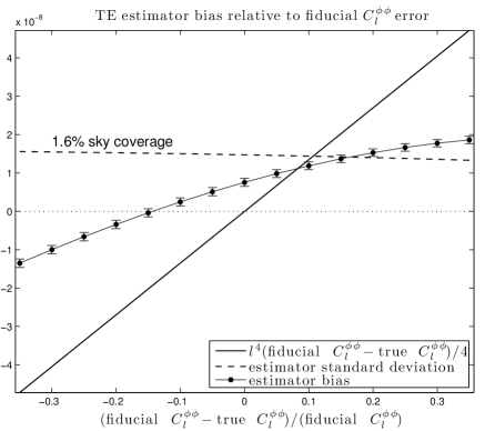
Figure 5: Spectral estimation bias averaged over the multiple bin $l\in[10,200]$ as a function of fiducial uncertainty. See Section VI for details.

VI Simulation

We perform two simulation experiments under experimental conditions similar to those found in future ACTpol/SPTpol experiments. The first simulation explores the bias terms $N^{(j)}_{{\bm{l}}}$ and $\bigl{\langle}N^{(j)}_{{\bm{l}},\text{\tiny obs}}\bigr{\rangle}$ for the two quadratic estimators $\hat{\phi}^{\text{\tiny$X\!Y$}}_{\bm{l}}$ and $\tilde{\phi}^{\text{\tiny$X\!Y$}}_{\bm{l}}$. The results are summarized in figures 1, 2 and 3. For these simulations, to compute the lensed weights in $\tilde{\phi}^{\text{\tiny$X\!Y$}}_{\bm{l}}$, we use the same fiducial model for $C_{\bm{l}}^{\phi\phi}$ as the simulation model for $C_{\bm{l}}^{\phi\phi}$. In contrast, for the second set of simulations we explore the effect of uncertainty in the fiducial model for $C_{\bm{l}}^{\phi\phi}$ when computing $\tilde{\phi}^{\text{\tiny$X\!Y$}}_{\bm{l}}$. The results are summarized in figures 4, 5 and 6. The main conclusion of the first set of simulations is that although $\tilde{\phi}^{\text{\tiny$X\!Y$}}_{\bm{l}}$ does reduce low $l$ estimation bias, this is accomplished by increasing $N^{(1)}_{{\bm{l}}}$ (or $\bigl{\langle}N^{(1)}_{{\bm{l}},\text{\tiny obs}}\bigr{\rangle}$ in the case that one uses $N^{(0)}_{{\bm{l}},\text{\tiny obs}}$ instead of $N^{(0)}_{{\bm{l}}}$) to the point of canceling with $N^{(2)}_{{\bm{l}}}$ (or $\bigl{\langle}N^{(2)}_{{\bm{l}},\text{\tiny obs}}\bigr{\rangle}$ as the case may be) when the correct model for $C_{\bm{l}}^{\phi\phi}$ is used to generate the lensed weights. The second set of simulations show that this cancelation can be sensitive to the fiducial model for $C_{\bm{l}}^{\phi\phi}$ depending on which estimator one uses: TE and EE are most sensitive, EB is least sensitive. At the end of this section we discuss the inferential implications for future experiments.

The cosmology used in our simulations are based on a flat, power law $\Lambda$CDM cosmological model, with baryon density $\Omega_{b}=0.044$; cold dark matter density $\Omega_{\text{cdm}}=0.21$; cosmological constant density $\Omega_{\Lambda}=0.74$; Hubble parameter $h=0.71$ in units of 100 km s${}^{-1}\,$Mpc^-1; primordial scalar fluctuation amplitude $A_{s}(k=0.002\,$Mpc${}^{-1})=2.45\times 10^{-9}$; scalar spectral index $n_{s}(k=0.002\,$Mpc${}^{-1})=0.96$; primordial helium abundance $Y_{P}=0.24$; and reionization optical depth $\tau_{r}=0.088$. The CAMB code is used to generate the theoretical power spectra Lewis et al. (2000).

To construct the lensed CMB simulation we first generate a high resolution simulation of $\Theta(\bm{x})$ and the gravitational potential $\phi(\bm{x})$ on a periodic $25.6^{\text{o}}\times 25.6^{\text{o}}$ patch of the flat sky. The lensing operation is performed by taking the numerical gradient of $\phi$, then using linear interpolation to obtain the lensed field $\Theta(\bm{x}+\nabla\phi(\bm{x}))$. We down-sample the lensed field to obtain the desired 1.5 arcmin pixel resolution for the simulation output. Finally, the observational noise (with a standard deviation of $5\mu$K-arcmin on $T$ and $\sqrt{2}\times 5\mu$K-arcmin on $E$, $B$ and Gaussian beam FWHM=1.5 arcmin deconvolution) is added in Fourier space. For all of the simulations we assume a zero $B$ mode and a lensing potential $\phi$ which is uncorrelated with the CMB. In contrast to the full lensing simulation, the pertabive expansions given in Section V.1 only require simulation of unlensed CMB fields at the low resolution 1.5 arcmin pixels.

Figures 1, 2 and 3

Each plot in figures 1, 2 and 3 correspond to a different quadratic pairing $X,Y\in\{T,E,B\}$ and shows the Monte Carlo approximations to $l^{4}\bigl{\langle}N^{(1)}_{{\bm{l}},\text{\tiny obs}}\bigr{\rangle}/4$ and $l^{4}\bigl{\langle}N^{(2)}_{{\bm{l}},\text{\tiny obs}}\bigr{\rangle}/4$ along with the expected value of the spectral density estimates $l^{4}(\delta_{0}^{-1}|\hat{\phi}_{\bm{l}}^{\text{\tiny$X\!Y$}}|^{2}-N^{(0)}_{{\bm{l}},\text{\tiny obs}})/4$ and $l^{4}(\delta_{0}^{-1}|\tilde{\phi}_{\bm{l}}^{\text{\tiny$X\!Y$}}|^{2}-N^{(0)}_{{\bm{l}},\text{\tiny obs}})/4$ over different realizations of $\phi$, the CMB and the observational noise. Although not shown, the bias terms $l^{4}N^{(1)}_{{\bm{l}}}/4$ were also computed, using the coupling technique given in Section V.2, and resulted in very similar plots (mostly indistinguishable above the Monte Carlo error). The spectral density estimates are computed from the all-order lensed simulations whereas the bias terms are computed using perturbative expansions discussed in Section V.1. The Monte Carlo approximations are based on 2000 independent realizations for the $TT$, $EE$ and $EB$ estimators and 18000 independent realizations for the $TE$ and $TB$ estimators. These estimates are then radially averaged on sliding concentric annuli with wavenumber bins of width $20$ to yield the plots shown in figures 1, 2 and 3.

The main feature in these simulations is the large increase in $\bigl{\langle}N^{(1)}_{{\bm{l}},\text{\tiny obs}}\bigr{\rangle}$ bias at low $l$ for $\tilde{\phi}^{\text{\tiny$X\!Y$}}_{\bm{l}}$ as compared to the corresponding quantity for $\hat{\phi}^{\text{\tiny$X\!Y$}}_{\bm{l}}$, especially for the EE, TE and TT estimators. In contrast, $\bigl{\langle}N^{(2)}_{{\bm{l}},\text{\tiny obs}}\bigr{\rangle}$ also increases in magnitude but to a lesser extent, enabling the cancelation with $\bigl{\langle}N^{(1)}_{{\bm{l}},\text{\tiny obs}}\bigr{\rangle}$. Since the terms $\bigl{\langle}N^{(1)}_{{\bm{l}},\text{\tiny obs}}\bigr{\rangle}$ and $\bigl{\langle}N^{(2)}_{{\bm{l}},\text{\tiny obs}}\bigr{\rangle}$ are not individually small but instead cancel, there is the potential for this cancelation to be offset when there is uncertainty in the fiducial model for $C_{\bm{l}}^{\phi\phi}$ used to compute the lensing weights for the estimate $\tilde{\phi}^{\text{\tiny$X\!Y$}}_{\bm{l}}$. In the next section we explore this sensitivity by analyzing the resulting estimation bias as a function of fiducial sensitivity.

Figures 4, 5 and 6

To explore the effect of fiducial uncertainty when computing the lensed weights in $\tilde{\phi}^{\text{\tiny$X\!Y$}}_{\bm{l}}$ we fixed a fiducial model $C_{\bm{l}}^{\phi\phi}$ used to compute the lensed weights, then analyzed simulations under perturbations of $C_{\bm{l}}^{\phi\phi}$. In particular, we considered simulation models which differ from the fiducial model by a maximum of $35$% only in the multipole range $[10,200]$. The simulation models are of the form $T_{\bm{l}}C_{\bm{l}}^{\phi\phi}$ where $T_{\bm{l}}=1$ when $l\notin[10,200]$ and $T_{\bm{l}}=c$ when $l\in[10,200]$ where $c$ ranges from $1.35$ to $0.65$. For each scalar $c$ we simulated 200 different CMB, lensing and noise fields. At each simulation we recorded the estimation error, namely $l^{4}\bigl{(}\delta_{0}^{-1}|\tilde{\phi}_{\bm{l}}^{\text{\tiny$X\!Y$}}|^{2}-N^{(0)}_{{\bm{l}},\text{\tiny obs}}-T_{\bm{l}}C_{\bm{l}}^{\phi\phi}\bigr{)}/4$, averaged over all frequencies in the $l$ bin $[10,200]$. This error is then averaged all $200$ simulations to estimate the bias. This bias is then plotted for each quadratic pairing $X,Y\in\{T,E,B\}$ in figures 4, 5 and 6. The estimation bias is shown as ‘$-\!\!\bullet\!\!-$’ with $1\sigma$ monte carlo error bars attached as a function of the fiducial uncertainty $1-c$ in the bin $l\in[10,200]$. The dashed line shows the standard deviation of $l^{4}(\delta_{0}^{-1}|\tilde{\phi}_{\bm{l}}^{\text{\tiny$X\!Y$}}|^{2}-N^{(0)}_{{\bm{l}},\text{\tiny obs}})/4$ and the solid black line plots the fiducial error $(1-T_{\bm{l}})l^{4}C_{\bm{l}}^{\phi\phi}/4$ averaged over $l\in[10,200]$.

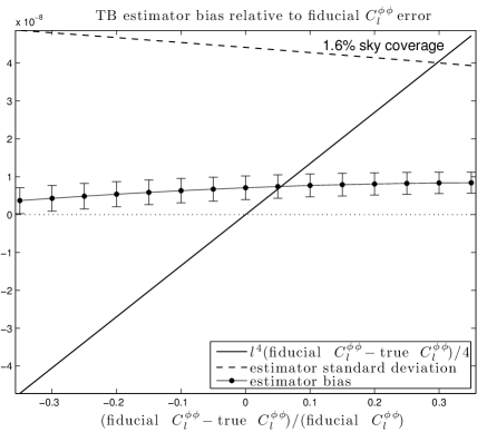
Figure 6: Spectral estimation bias averaged over the multiple bin $l\in[10,200]$ as a function of fiducial uncertainty. See Section VI for details.

Does this effect future inference?

Table 1 summarizes fiducial uncertainty (at 15%), estimation standard deviation, and bias range when using $\tilde{\phi}_{\bm{l}}^{\text{\tiny$X\!Y$}}$ to estimate the average power in $l^{4}C_{\bm{l}}^{\phi\phi}/4$ over $l\in[10,200]$. Each row corresponds to a different quadratic pairing $X,Y\in\{T,E,B\}$. The second column shows the bias range corresponding to $15$% fiducial uncertainty taken from figures 4, 5 and 6. We list bias range, versus absolute bias, since any baseline bias can be estimated with simulation and subsequently subtracted from any estimate. The third column shows $4\sigma$ full sky error bars where the estimation standard deviation is extrapolated from figures 4, 5 and 6 to full sky $\sigma$ by multiplying $\sqrt{f_{\text{sky}}}=0.126$. Notice that, ignoring the bias, the $EE$ and $EB$ estimator have the power to constrain the fiducial uncertainty by a factor of $3$. However, accounting for bias this constraining power is mitigated, especially for estimators $EE$ and $TE$. In contrast, the $EB$ estimator bias can nearly ignored completely.

$\tilde{\phi}_{\bm{l}}^{\text{\tiny$X\!Y$}}$	$\sim$ bias range	$\sim$ full sky $4\sigma$	fiducial error ($15\%$)
TE	$\pm 0.70$	$\pm 0.76$	$\pm 2.02$
EE	$\pm 0.53$	$\pm 0.62$	$\pm 2.02$
TT	$\pm 0.16$	$\pm 0.86$	$\pm 2.02$
TB	$\pm 0.10$	$\pm 2.33$	$\pm 2.02$
EB	$\pm 0.01$	$\pm 0.67$	$\pm 2.02$

Table 1: In units of spectral power, per $10^{-8}$, the above table shows bias range, approximate full sky standard deviation and fiducial error (at 15%) for each quadratic estimate $\tilde{\phi}_{\bm{l}}^{\text{\tiny$T\!E$}}$, $\tilde{\phi}_{\bm{l}}^{\text{\tiny$E\!E$}}$, $\tilde{\phi}_{\bm{l}}^{\text{\tiny$T\!T$}}$, $\tilde{\phi}_{\bm{l}}^{\text{\tiny$T\!B$}}$ and $\tilde{\phi}_{\bm{l}}^{\text{\tiny$E\!B$}}$.

VII Discussion

The state-of-the-art estimator of weak lensing, the quadratic estimator developed by Hu and Okomoto Hu (2001); Hu and Okamoto (2002), works in part through a delicate cancelation of terms in a Taylor expansion of the lensing effect on the CMB. In this paper we present two simulation based approaches for exploring the nature of this cancelation for both the CMB intensity and the polarization fields. In particular, we use these two simulation algorithms to analyze the so called $N^{(1)}_{\bm{l}}$ and $N^{(2)}_{\bm{l}}$ bias for two modifications of the full set of quadratic temperature/polarization lensing estimators: one which incorporates lensed rather than unlensed spectra into the estimator weights to mitigate the effect of higher order terms; and one which uses the observed lensed CMB fields to correct for the, so called, $N^{(0)}_{\bm{l}}$ bias. Our simulation algorithms, which can simulate all higher order bias terms $N^{(j)}_{\bm{l}}$ for $j\geq 0$, utilize an extension of the FFT techniques developed in Hu (2001). These FFT characterizations are key to making estimates of the $N^{(j)}_{\bm{l}}$ fast and additionally provide fast (non-stochastic) algorithms for approximating the $N^{(0)}_{\bm{l}}$ bias using the observed lensed CMB fields.

In Section VI we use our algorithm to analyze the modified quadratic temperature/polarization lensing estimators for future ACTpol/SPTpol experiments. We find that the modified estimates do reduce low $l$ estimation bias. However this is accomplished by effectively increasing the magnitude of $N^{(1)}_{{\bm{l}}}$ and $N^{(2)}_{{\bm{l}}}$ to the point of cancelation when the correct model for $C_{\bm{l}}^{\phi\phi}$ is used to generate the lensed weights. We also demonstrate, through an analysis of estimator bias versus fiducial uncertainty, that this cancelation can be sensitive to the fiducial model for $C_{\bm{l}}^{\phi\phi}$ depending on which estimator one uses: TE and EE are most sensitive, EB is least sensitive. For low $l$ estimation in future ACTpol/SPTpol experiments we conclude that the bias in the EB estimator can be effectively ignored. For the TE and the EE estimators, however, the bias does contribute significantly to projected error bars and may need to be corrected to give the estimator inferential power beyond a nominal fiducial uncertainty.

Appendix A FFT algorithms

In this section we derive the FFT algorithms which allow fast simulation of the fields $\mathscr{L}^{(j)}_{\bm{l}}$, $\mathscr{O}^{(j)}_{\bm{l}}$ and $\mathscr{N}^{(j)}_{{\bm{l}}}$ as described in Section V.1. We begin with some notational conventions which greatly simplify the subsequent formulas. First let $\varphi_{\bm{k}}$ denote the phase angle of frequency ${\bm{k}}$ and $\Delta\varphi\equiv\varphi_{{\bm{k}}+{\bm{l}}}-\varphi_{{\bm{k}}}$. Also let $l_{a}$ denote the $a^{\text{th}}$ coordinate of ${\bm{l}}$. For any field $X\in\{T,E,B\}$ we let

$$\hat{X}_{\bm{k}}\equiv e^{i2\varphi_{\bm{k}}}X_{\bm{k}},\qquad\check{X}_{\bm{k}}\equiv e^{i4\varphi_{\bm{k}}}X_{\bm{k}}.$$

Furthermore, we will utilize a super-script/sub-script notation to denote multiplication/division by particular power spectra. An example serves to illustrate the notation:

$$\bigl{(}\check{X}_{\text{\tiny$T\!T$}}\bigr{)}_{\bm{k}} \equiv\check{X}_{\bm{k}}\frac{1}{\widetilde{C}_{{\bm{k}},\text{\tiny exp}}^{\text{\tiny$T\!T$}}},\qquad\bigl{(}\check{X}_{\text{\tiny$T\!T$},\text{\tiny$E\!E$}}^{\text{\tiny$T\!E$}}\bigr{)}_{\bm{k}}\equiv\check{X}_{\bm{k}}\frac{C_{\bm{k}}^{\text{\tiny$T\!E$}}}{\widetilde{C}_{{\bm{k}},\text{\tiny exp}}^{\text{\tiny$T\!T$}}\widetilde{C}_{{\bm{k}},\text{\tiny exp}}^{\text{\tiny$E\!E$}}}$$

$$\bigl{(}\check{X}_{\text{\tiny$T\!T$}}^{\text{\tiny$T\!E$}}\bigr{)}_{\bm{k}} \equiv\check{X}_{\bm{k}}\frac{C_{\bm{k}}^{\text{\tiny$T\!E$}}}{\widetilde{C}_{{\bm{k}},\text{\tiny exp}}^{\text{\tiny$T\!T$}}},\qquad\bigl{(}\check{X}_{\text{\tiny$T\!T$},\text{\tiny$E\!E$}}^{\text{\tiny$T\!E$},\text{\tiny$T\!T$}}\bigr{)}_{\bm{k}}\equiv\check{X}_{\bm{k}}\frac{C_{\bm{k}}^{\text{\tiny$T\!E$}}C_{\bm{k}}^{\text{\tiny$T\!T$}}}{\widetilde{C}_{{\bm{k}},\text{\tiny exp}}^{\text{\tiny$T\!T$}}\widetilde{C}_{{\bm{k}},\text{\tiny exp}}^{\text{\tiny$E\!E$}}}.$$

Notice that the above denominators always use lensed spectra with experimental noise, whereas the numerators always use unlensed spectra. In doing so, the formulas found in claims 1 through 5 below can be used for fast algorithms for the quadratic estimate $\hat{\phi}_{\bm{l}}^{\text{\tiny$X\!Y$}}$. To obtain the corresponding formulas for the modified quadratic estimate $\tilde{\phi}^{\text{\tiny$X\!Y$}}_{\bm{l}}$ one simply needs to replace the unlensed spectra in the numerator of the above notation, with the lensed spectra (but without experimental noise).

Claim 1 (TT estimator)

If $X_{\bm{k}}$ and $Y_{\bm{k}}$ are complex functions such that $X_{-{\bm{k}}}=X^{*}_{\bm{k}}$ and $Y_{-{\bm{k}}}=Y^{*}_{\bm{k}}$ then

$$\int\frac{d^{2}\bm{k}}{2\pi}g^{\text{\tiny$T\!T$}}_{\bm{l},\bm{k}\,}X_{\bm{k}+\bm{l}}Y^{*}_{\bm{k}} =-il_{a}\int\frac{d^{2}{\bm{x}}}{2\pi}e^{-i{\bm{l}}\cdot{\bm{x}}}$$

$$\times\Bigl{(}[\nabla^{a}X_{\text{\tiny$T\!T$}}^{\text{\tiny$T\!T$}}({\bm{x}})][Y_{\text{\tiny$T\!T$}}({\bm{x}})]$$

$$\quad+[\nabla^{a}Y_{\text{\tiny$T\!T$}}^{\text{\tiny$T\!T$}}({\bm{x}})][X_{\text{\tiny$T\!T$}}({\bm{x}})]\Bigr{)};$$

$$\int\frac{d^{2}{\bm{k}}}{(2\pi)^{2}}|g^{\text{\tiny T\!T}}_{{\bm{l}},{\bm{k}}\,}|^{2}X_{{\bm{k}}+{\bm{l}}}Y^{*}_{{\bm{k}}} =-\frac{l_{a}l_{b}}{2\pi}\int\frac{d^{2}{\bm{x}}}{2\pi}e^{-i{\bm{l}}\cdot{\bm{x}}}$$

$$\times\Bigl{(}2[\nabla^{a}X^{\text{\tiny$T\!T$}}_{\text{\tiny$T\!T$},\text{\tiny$T\!T$}}({\bm{x}})][\nabla^{b}Y^{\text{\tiny$T\!T$}}_{\text{\tiny$T\!T$},\text{\tiny$T\!T$}}({\bm{x}})]$$

$$\quad+[X_{\text{\tiny$T\!T$},\text{\tiny$T\!T$}}({\bm{x}})][\nabla^{a}\nabla^{b}Y^{\text{\tiny$T\!T$},\text{\tiny$T\!T$}}_{\text{\tiny$T\!T$},\text{\tiny$T\!T$}}({\bm{x}})]$$

$$\quad+[Y_{\text{\tiny$T\!T$},\text{\tiny$T\!T$}}({\bm{x}})][\nabla^{a}\nabla^{b}X^{\text{\tiny$T\!T$},\text{\tiny$T\!T$}}_{\text{\tiny$T\!T$},\text{\tiny$T\!T$}}({\bm{x}})]\Bigr{)};$$

$$\int\frac{d^{2}{\bm{k}}}{(2\pi)^{2}}g^{\text{\tiny$T\!T$}}_{{\bm{l}},{\bm{k}}\,}g^{\text{\tiny$T\!T$}}_{{\bm{l}},-{\bm{k}}-{\bm{l}}\,}X_{{\bm{k}}+{\bm{l}}}Y^{*}_{{\bm{k}}}=\int\frac{d^{2}{\bm{k}}}{(2\pi)^{2}}|g^{\text{\tiny T\!T}}_{{\bm{l}},{\bm{k}}\,}|^{2}X_{{\bm{k}}+{\bm{l}}}Y^{*}_{{\bm{k}}},$$

where $g^{\text{\tiny$T\!T$}}_{{\bm{l}},{\bm{k}}\,}\equiv 2\pi{f^{\text{\tiny$T\!T$}}_{{\bm{l}},{\bm{k}}}}[\widetilde{C}^{\text{\tiny$T\!T$}}_{{\bm{k}}+{\bm{l}},\text{\tiny exp}}\widetilde{C}^{\text{\tiny$T\!T$}}_{{\bm{k}},\text{\tiny exp}}]^{-1}$ and $f^{\text{\tiny$TT$}}_{{\bm{l}},{\bm{k}}}\equiv\frac{1}{2\pi}[{\bm{l}}\cdot({\bm{k}}+{\bm{l}})C^{\text{\tiny$TT$}}_{{\bm{k}}+{\bm{l}}}-{\bm{l}}\cdot{\bm{k}}C^{\text{\tiny$TT$}}_{{\bm{k}}}]$.

Claim 2 (TE estimator)

If $X_{\bm{k}}$ and $Y_{\bm{k}}$ are complex functions such that $X_{-{\bm{k}}}=X^{*}_{\bm{k}}$ and $Y_{-{\bm{k}}}=Y^{*}_{\bm{k}}$ then

$$\int\frac{d^{2}\bm{k}}{2\pi}g^{\text{\tiny$T\!E$}}_{\bm{l},\bm{k}\,}X_{\bm{k}+\bm{l}}Y^{*}_{\bm{k}} =-il_{a}\int\frac{d^{2}{\bm{x}}}{2\pi}e^{-i{\bm{l}}\cdot{\bm{x}}}$$

$$\times\Bigl{(}Re\{[\nabla^{a}\hat{X}^{\text{\tiny$T\!E$}}_{\text{\tiny$T\!T$}}({\bm{x}})][\hat{Y}_{\text{\tiny$E\!E$}}({\bm{x}})]^{*}\}$$

$$\quad+[\nabla^{a}Y^{\text{\tiny$T\!E$}}_{\text{\tiny$E\!E$}}({\bm{x}})][X_{\text{\tiny$T\!T$}}({\bm{x}})]\Bigr{)};$$

$$\int\frac{d^{2}{\bm{k}}}{(2\pi)^{2}} |g^{\text{\text{\tiny$T\!E$} }}_{{\bm{l}},{\bm{k}}\,}|^{2}X_{{\bm{k}}+{\bm{l}}}Y^{*}_{{\bm{k}}}=-\frac{l_{a}l_{b}}{4\pi}\int\frac{d^{2}{\bm{x}}}{2\pi}e^{-i{\bm{l}}\cdot{\bm{x}}}$$

$$\times\Bigl{(}[Y_{\text{\tiny$E\!E$},\text{\tiny$E\!E$}}({\bm{x}})][\nabla^{a}\nabla^{b}X^{\text{\tiny$T\!E$},\text{\tiny$T\!E$}}_{\text{\tiny$T\!T$},\text{\tiny$T\!T$}}({\bm{x}})]$$

$$\quad+Re\{[\check{Y}_{\text{\tiny$E\!E$},\text{\tiny$E\!E$}}({\bm{x}})][\nabla^{a}\nabla^{b}\check{X}^{\text{\tiny$T\!E$},\text{\tiny$T\!E$}}_{\text{\tiny$T\!T$},\text{\tiny$T\!T$}}({\bm{x}})]^{*}\}$$

$$\quad+2[X_{\text{\tiny$T\!T$},\text{\tiny$T\!T$}}({\bm{x}})][\nabla^{a}\nabla^{b}Y^{\text{\tiny$T\!E$},\text{\tiny$T\!E$}}_{\text{\tiny$E\!E$},\text{\tiny$E\!E$}}({\bm{x}})]$$

$$\quad+Re\{4[\nabla^{a}\hat{X}^{\text{\tiny$T\!E$}}_{\text{\tiny$T\!T$},\text{\tiny$T\!T$}}({\bm{x}})][\nabla^{b}\hat{Y}^{\text{\tiny$T\!E$}}_{\text{\tiny$E\!E$},\text{\tiny$E\!E$}}({\bm{x}})]^{*}\}\Bigr{)};$$

$$\int\frac{d^{2}{\bm{k}}}{(2\pi)^{2}}g^{\text{\tiny$T\!E$}}_{{\bm{l}},{\bm{k}}\,} g^{\text{\tiny$T\!E$}}_{{\bm{l}},-{\bm{k}}-{\bm{l}}\,}X_{{\bm{k}}+{\bm{l}}}Y^{*}_{{\bm{k}}}=-\frac{l_{a}l_{b}}{4\pi}\int\frac{d^{2}{\bm{x}}}{2\pi}e^{-i{\bm{l}}\cdot{\bm{x}}}$$

$$\times\Bigl{(}Re\{2[\nabla^{a}\nabla^{b}\hat{X}^{\text{\tiny$T\!E$},\text{\tiny$T\!E$}}_{\text{\tiny$T\!T$},\text{\tiny$E\!E$}}({\bm{x}})][\hat{Y}_{\text{\tiny$T\!T$},\text{\tiny$E\!E$}}({\bm{x}})]^{*}\}$$

$$\quad+Re\{2[\nabla^{a}\nabla^{b}\hat{Y}^{\text{\tiny$T\!E$},\text{\tiny$T\!E$}}_{\text{\tiny$T\!T$},\text{\tiny$E\!E$}}({\bm{x}})][\hat{X}_{\text{\tiny$T\!T$},\text{\tiny$E\!E$}}({\bm{x}})]^{*}\}$$

$$\quad+3[\nabla^{a}X^{\text{\tiny$T\!E$}}_{\text{\tiny$T\!T$},\text{\tiny$E\!E$}}({\bm{x}})][\nabla^{b}Y^{\text{\tiny$T\!E$}}_{\text{\tiny$T\!T$},\text{\tiny$E\!E$}}({\bm{x}})]$$

$$\quad+Re\{[\nabla^{b}\check{Y}^{\text{\tiny$T\!E$}}_{\text{\tiny$T\!T$},\text{\tiny$E\!E$}}({\bm{x}})][\nabla^{a}\check{X}^{\text{\tiny$T\!E$}}_{\text{\tiny$T\!T$},\text{\tiny$E\!E$}}({\bm{x}})]^{*}\}\Bigr{)},$$

where $g^{\text{\tiny$T\!E$}}_{{\bm{l}},{\bm{k}}\,}\equiv 2\pi{f^{\text{\tiny$T\!E$}}_{{\bm{l}},{\bm{k}}}}[\widetilde{C}^{\text{\tiny$T\!T$}}_{{\bm{k}}+{\bm{l}},\text{\tiny exp}}\widetilde{C}^{\text{\tiny$E\!E$}}_{{\bm{k}},\text{\tiny exp}}]^{-1}$ and $f^{\text{\tiny$T\!E$}}_{{\bm{l}},{\bm{k}}}\equiv\frac{1}{2\pi}[{\bm{l}}\cdot({\bm{k}}+{\bm{l}})\cos(2\Delta\varphi)C^{\text{\tiny$T\!E$}}_{{\bm{k}}+{\bm{l}}}-{\bm{l}}\cdot{\bm{k}}C^{\text{\tiny$T\!E$}}_{{\bm{k}}}]$.

Claim 3 (TB estimator)

If $X_{\bm{k}}$ and $Y_{\bm{k}}$ are complex functions such that $X_{-{\bm{k}}}=X^{*}_{\bm{k}}$ and $Y_{-{\bm{k}}}=Y^{*}_{\bm{k}}$ then

$$\int\frac{d^{2}\bm{k}}{2\pi}g^{\text{\tiny$T\!B$}}_{\bm{l},\bm{k}\,}X_{\bm{k}+\bm{l}}Y^{*}_{\bm{k}} =-il_{a}\int\frac{d^{2}{\bm{x}}}{2\pi}e^{-i{\bm{l}}\cdot{\bm{x}}}$$

$$\quad\times Im\{[\nabla^{a}\hat{X}^{\text{\tiny$T\!E$}}_{\text{\tiny$T\!T$}}({\bm{x}})][\hat{Y}_{\text{\tiny$B\!B$}}({\bm{x}})]^{*}\};$$

$$\int\frac{d^{2}{\bm{k}}}{(2\pi)^{2}} |g^{\text{\tiny$T\!B$}}_{{\bm{l}},{\bm{k}}\,}|^{2}X_{{\bm{k}}+{\bm{l}}}Y^{*}_{{\bm{k}}}=-\frac{l_{a}l_{b}}{4\pi}\int\frac{d^{2}{\bm{x}}}{2\pi}e^{-i{\bm{l}}\cdot{\bm{x}}}$$

$$\times\Bigl{(}[Y_{\text{\tiny$B\!B$},\text{\tiny$B\!B$}}({\bm{x}})][\nabla^{a}\nabla^{b}X^{\text{\tiny$T\!E$},\text{\tiny$T\!E$}}_{\text{\tiny$T\!T$},\text{\tiny$T\!T$}}({\bm{x}})]$$

$$\quad-Re\{[\check{Y}_{\text{\tiny$B\!B$},\text{\tiny$B\!B$}}({\bm{x}})][\nabla^{a}\nabla^{b}\check{X}^{\text{\tiny$T\!E$},\text{\tiny$T\!E$}}_{\text{\tiny$T\!T$},\text{\tiny$T\!T$}}({\bm{x}})]^{*}\}\Bigr{)};$$

$$\int\frac{d^{2}{\bm{k}}}{(2\pi)^{2}}g^{\text{\tiny$T\!B$}}_{{\bm{l}},{\bm{k}}\,} g^{\text{\tiny$T\!B$}}_{{\bm{l}},-{\bm{k}}-{\bm{l}}\,}X_{{\bm{k}}+{\bm{l}}}Y^{*}_{{\bm{k}}}=-\frac{l_{a}l_{b}}{4\pi}\int\frac{d^{2}{\bm{x}}}{2\pi}e^{-i{\bm{l}}\cdot{\bm{x}}}$$

$$\times\Bigl{(}[\nabla^{a}X^{\text{\tiny$T\!E$}}_{\text{\tiny$T\!T$},\text{\tiny$B\!B$}}({\bm{x}})][\nabla^{b}Y^{\text{\tiny$T\!E$}}_{\text{\tiny$T\!T$},\text{\tiny$B\!B$}}({\bm{x}})]$$

$$\quad-Re\{[\nabla^{a}\check{X}^{\text{\tiny$T\!E$}}_{\text{\tiny$T\!T$},\text{\tiny$B\!B$}}({\bm{x}})][\nabla^{b}\check{Y}^{\text{\tiny$T\!E$}}_{\text{\tiny$T\!T$},\text{\tiny$B\!B$}}({\bm{x}})]^{*}\}\Bigr{)},$$

where $g^{\text{\tiny$T\!B$}}_{{\bm{l}},{\bm{k}}\,}\equiv 2\pi{f^{\text{\tiny$T\!B$}}_{{\bm{l}},{\bm{k}}}}[\widetilde{C}^{\text{\tiny$T\!T$}}_{{\bm{k}}+{\bm{l}},\text{\tiny exp}}\widetilde{C}^{\text{\tiny$B\!B$}}_{{\bm{k}},\text{\tiny exp}}]^{-1}$ and $f^{\text{\tiny$T\!B$}}_{{\bm{l}},{\bm{k}}}\equiv\frac{1}{2\pi}[{\bm{l}}\cdot({\bm{k}}+{\bm{l}})C^{\text{\tiny$T\!E$}}_{{\bm{k}}+{\bm{l}}}]\sin(2\Delta\varphi)$.

Claim 4 (EB estimator)

If $X_{\bm{k}}$ and $Y_{\bm{k}}$ are complex functions such that $X_{-{\bm{k}}}=X^{*}_{\bm{k}}$ and $Y_{-{\bm{k}}}=Y^{*}_{\bm{k}}$ then

$$\int\frac{d^{2}\bm{k}}{2\pi}g^{\text{\tiny$E\!B$}}_{\bm{l},\bm{k}\,}X_{\bm{k}+\bm{l}}Y^{*}_{\bm{k}} =-il_{a}\int\frac{d^{2}{\bm{x}}}{2\pi}e^{-i{\bm{l}}\cdot{\bm{x}}}$$

$$\quad\times Im\{[\nabla^{a}\hat{X}^{\text{\tiny$E\!E$}}_{\text{\tiny$E\!E$}}({\bm{x}})][\hat{Y}_{\text{\tiny$B\!B$}}({\bm{x}})]^{*}\};$$

$$\int\frac{d^{2}{\bm{k}}}{(2\pi)^{2}}|g^{\text{\tiny$E\!B$}}_{{\bm{l}},{\bm{k}}\,}|^{2} X_{{\bm{k}}+{\bm{l}}}Y^{*}_{{\bm{k}}}=-\frac{l_{a}l_{b}}{4\pi}\int\frac{d^{2}{\bm{x}}}{2\pi}e^{-i{\bm{l}}\cdot{\bm{x}}}$$

$$\times\Bigl{(}[Y_{\text{\tiny$B\!B$},\text{\tiny$B\!B$}}({\bm{x}})][\nabla^{a}\nabla^{b}X^{\text{\tiny$E\!E$},\text{\tiny$E\!E$}}_{\text{\tiny$E\!E$},\text{\tiny$E\!E$}}({\bm{x}})]$$

$$\quad-Re\{[\check{Y}_{\text{\tiny$B\!B$},\text{\tiny$B\!B$}}({\bm{x}})][\nabla^{a}\nabla^{b}\check{X}^{\text{\tiny$E\!E$},\text{\tiny$E\!E$}}_{\text{\tiny$E\!E$},\text{\tiny$E\!E$}}({\bm{x}})]^{*}\}\Bigr{)};$$

$$\int\frac{d^{2}{\bm{k}}}{(2\pi)^{2}}g^{\text{\tiny$E\!B$}}_{{\bm{l}},{\bm{k}}\,} g^{\text{\tiny$E\!B$}}_{{\bm{l}},-{\bm{k}}-{\bm{l}}\,}X_{{\bm{k}}+{\bm{l}}}Y^{*}_{{\bm{k}}}=-\frac{l_{a}l_{b}}{4\pi}\int\frac{d^{2}{\bm{x}}}{2\pi}e^{-i{\bm{l}}\cdot{\bm{x}}}$$

$$\times\Bigl{(}[\nabla^{a}X^{\text{\tiny$E\!E$}}_{\text{\tiny$E\!E$},\text{\tiny$B\!B$}}({\bm{x}})][\nabla^{b}Y^{\text{\tiny$E\!E$}}_{\text{\tiny$E\!E$},\text{\tiny$B\!B$}}({\bm{x}})]$$

$$\quad-Re\{[\nabla^{a}\check{X}^{\text{\tiny$E\!E$}}_{\text{\tiny$E\!E$},\text{\tiny$B\!B$}}({\bm{x}})][\nabla^{b}\check{Y}^{\text{\tiny$E\!E$}}_{\text{\tiny$E\!E$},\text{\tiny$B\!B$}}({\bm{x}})]^{*}\}\Bigr{)},$$

where $g^{\text{\tiny$E\!B$}}_{{\bm{l}},{\bm{k}}\,}\equiv 2\pi{f^{\text{\tiny$E\!B$}}_{{\bm{l}},{\bm{k}}}}[\widetilde{C}^{\text{\tiny$E\!E$}}_{{\bm{k}}+{\bm{l}},\text{\tiny exp}}\widetilde{C}^{\text{\tiny$B\!B$}}_{{\bm{k}},\text{\tiny exp}}]^{-1}$ and $f^{\text{\tiny$E\!B$}}_{{\bm{l}},{\bm{k}}}\equiv\frac{1}{2\pi}[{\bm{l}}\cdot({\bm{k}}+{\bm{l}})C^{\text{\tiny$E\!E$}}_{{\bm{k}}+{\bm{l}}}]\sin(2\Delta\varphi)$.

Claim 5 (EE estimator)

If $X_{\bm{k}}$ and $Y_{\bm{k}}$ are complex functions such that $X_{-{\bm{k}}}=X^{*}_{\bm{k}}$ and $Y_{-{\bm{k}}}=Y^{*}_{\bm{k}}$ then

$$\int\frac{d^{2}\bm{k}}{2\pi}g^{\text{\tiny$E\!E$}}_{\bm{l},\bm{k}\,}X_{\bm{k}+\bm{l}}Y^{*}_{\bm{k}} =-il_{a}\int\frac{d^{2}{\bm{x}}}{2\pi}e^{-i{\bm{l}}\cdot{\bm{x}}}$$

$$\times\Bigl{(}Re\{[\nabla^{a}\hat{X}^{\text{\tiny$E\!E$}}_{\text{\tiny$E\!E$}}({\bm{x}})][\hat{Y}_{\text{\tiny$E\!E$}}({\bm{x}})]^{*}\}$$

$$\quad+Re\{[\nabla^{a}\hat{Y}^{\text{\tiny$E\!E$}}_{\text{\tiny$E\!E$}}({\bm{x}})][\hat{X}_{\text{\tiny$E\!E$}}({\bm{x}})]^{*}\}\Bigr{)};$$

$$\int\frac{d^{2}{\bm{k}}}{(2\pi)^{2}}|g^{\text{\tiny$E\!E$}}_{{\bm{l}},{\bm{k}}\,}|^{2} X_{{\bm{k}}+{\bm{l}}}Y^{*}_{{\bm{k}}}=-\frac{l_{a}l_{b}}{4\pi}\int\frac{d^{2}{\bm{x}}}{2\pi}e^{-i{\bm{l}}\cdot{\bm{x}}}$$

$$\times\Bigl{(}[\nabla^{a}\nabla^{b}X^{\text{\tiny$E\!E$},\text{\tiny$E\!E$}}_{\text{\tiny$E\!E$},\text{\tiny$E\!E$}}({\bm{x}})][Y_{\text{\tiny$E\!E$},\text{\tiny$E\!E$}}({\bm{x}})]$$

$$\quad+Re\{[\nabla^{a}\nabla^{b}\check{X}^{\text{\tiny$E\!E$},\text{\tiny$E\!E$}}_{\text{\tiny$E\!E$},\text{\tiny$E\!E$}}({\bm{x}})][\check{Y}_{\text{\tiny$E\!E$},\text{\tiny$E\!E$}}({\bm{x}})]^{*}\}$$

$$\quad+[X_{\text{\tiny$E\!E$},\text{\tiny$E\!E$}}({\bm{x}})][\nabla^{a}\nabla^{b}Y^{\text{\tiny$E\!E$},\text{\tiny$E\!E$}}_{\text{\tiny$E\!E$},\text{\tiny$E\!E$}}({\bm{x}})]$$

$$\quad+Re\{[\check{X}_{\text{\tiny$E\!E$},\text{\tiny$E\!E$}}({\bm{x}})][\nabla^{a}\nabla^{b}\check{Y}^{\text{\tiny$E\!E$},\text{\tiny$E\!E$}}_{\text{\tiny$E\!E$},\text{\tiny$E\!E$}}({\bm{x}})]^{*}\}$$

$$\quad+2[\nabla^{a}X^{\text{\tiny$E\!E$}}_{\text{\tiny$E\!E$},\text{\tiny$E\!E$}}({\bm{x}})][\nabla^{b}Y^{\text{\tiny$E\!E$}}_{\text{\tiny$E\!E$},\text{\tiny$E\!E$}}({\bm{x}})]$$

$$\quad+Re\{2[\nabla^{a}\check{X}^{\text{\tiny$E\!E$}}_{\text{\tiny$E\!E$},\text{\tiny$E\!E$}}({\bm{x}})][\nabla^{b}\check{Y}^{\text{\tiny$E\!E$}}_{\text{\tiny$E\!E$},\text{\tiny$E\!E$}}({\bm{x}})]^{*}\}\Bigr{)};$$

$$\int\frac{d^{2}{\bm{k}}}{(2\pi)^{2}}g^{\text{\tiny$E\!E$}}_{{\bm{l}},{\bm{k}}\,}g^{\text{\tiny$E\!E$}}_{{\bm{l}},-{\bm{k}}-{\bm{l}}\,}X_{{\bm{k}}+{\bm{l}}}Y^{*}_{{\bm{k}}}=\int\frac{d^{2}{\bm{k}}}{(2\pi)^{2}}|g^{\text{\tiny$E\!E$}}_{{\bm{l}},{\bm{k}}\,}|^{2}X_{{\bm{k}}+{\bm{l}}}Y^{*}_{{\bm{k}}},$$

where $g^{\text{\tiny$E\!E$}}_{{\bm{l}},{\bm{k}}\,}\equiv 2\pi{f^{\text{\tiny$E\!E$}}_{{\bm{l}},{\bm{k}}}}[\widetilde{C}^{\text{\tiny$E\!E$}}_{{\bm{k}}+{\bm{l}},\text{\tiny exp}}\widetilde{C}^{\text{\tiny$E\!E$}}_{{\bm{k}},\text{\tiny exp}}]^{-1}$ and $f^{\text{\tiny$E\!E$}}_{{\bm{l}},{\bm{k}}}\equiv\frac{1}{2\pi}[{\bm{l}}\cdot({\bm{k}}+{\bm{l}})C^{\text{\tiny$EE$}}_{{\bm{k}}+{\bm{l}}}-{\bm{l}}\cdot{\bm{k}}C^{\text{\tiny$EE$}}_{{\bm{k}}}]\cos(2\Delta\varphi)$.

References

• Das et al. (2011) S. Das et al., Physical Review Letters, 107 (2011), doi:10.1103/PhysRevLett.107.021301.
• van Engelen et al. (2012) A. van Engelen et al.The Astrophysical Journal, 756, 142 (2012).
• Hu (2001) W. Hu, Astrophysics Journal, 557, L79 (2001), arXiv:astro-ph/0105424 .
• Hu and Okamoto (2002) W. Hu and T. Okamoto, Astrophysics Journal, 574, 566 (2002), arXiv:astro-ph/0111606 .
• Kesden et al. (2003) M. Kesden, A. Cooray,  and M. Kamionkowski, Physical Review D, 67 (2003), doi:10.1103/PhysRevD.67.123507.
• Hanson et al. (2011) D. Hanson, A. Challinor, G. Efstathiou,  and P. Bielewicz, Physical Review D, 83 (2011), doi:10.1103/PhysRevD.83.043005.
• Dodelson (2003) S. Dodelson, Modern cosmology (Academic Press, 2003).
• Lewis et al. (2000) A. Lewis, A. Challinor,  and A. Lasenby, The Astrophysical Journal, 538, 473 (2000).