Theoretical Modeling of the RR Lyrae Variables in NGC 1851

Abstract

The RR Lyrae instability strip (IS) in NGC 1851 is investigated, and a model is presented which reproduces the pulsational properties of the RR Lyrae population. In our model, a stellar component within the IS that displays minor helium variations ($Y$$\sim$0.248-0.270) is able to reproduce the observed periods and amplitudes of the RR Lyrae variables, as well as the frequency of fundamental and first-overtone RR Lyrae variables. The RR Lyrae variables therefore may belong to an He-enriched second generation of stars. The RR Lyrae variables with a slightly enhanced helium ($Y$$\sim$0.270-0.280) have longer periods at a given amplitude, as is seen with Oosterhoff II (OoII) RR Lyrae variables, whereas the RR Lyrae variables with $Y$$\sim$0.248-0.270 have shorter periods, exhibiting properties of Oosterhoff I (OoI) variables.

1 Introduction

The globular cluster (GC) NGC 1851 hosts two distinct subgiant branches (SGBs) (Milone et al., 2008), prompting much discussion as to the formation history of this cluster. The split between the bright SGB (SGBb) and faint SGB (SGBf) can be explained by two subpopulations that differ in age by about 1 Gyr (e.g., Milone et al., 2008; Gratton et al., 2012), or by two SGBs that are nearly coeval but have different C+N+O contents (e.g., Cassisi et al., 2008; Ventura et al., 2009). The horizontal branch (HB) of NGC 1851 also hosts two distinct populations, namely a prominent red HB clump and a blue tail. Finally, different populations have also been revealed in the red giant branch (RGB) (e.g., Grundahl et al., 1999; Han et al., 2009).

The HB of globular clusters (GCs) is a valuable stellar component which can be used to investigate the formation and evolution of GCs (e.g. Gratton et al., 2010; Dotter et al., 2010). Indeed, there have been previous studies to model the HB of the NGC 1851 to obtain scenarios of the formation this cluster’s bimodal horizontal branch (Salaris et al., 2008; Gratton et al., 2012). Our study concentrates on the portion of the HB inside the instability strip (IS), by discussing the case of the RR Lyrae properties in NGC 1851.

2 RR Lyrae Observations

Because of the compact nature NGC 1851, it is likely that the RR Lyrae star sample in the crowded core in incomplete (e.g. Sumerel et al., 2004; Downes et al., 2004). Fortunately at distances greater than 40” from the cluster center, individual stars can be relatively easily resolved, and there is no indication that the RR Lyrae sample is incomplete in this region. Therefore we limit our sample of RR Lyrae stars with which to compare our HB models to this outer region.

The outer RR Lyrae variables were studied by Walker (1998) using the $BVI$ passbands, and robust mean magnitudes, periods and amplitudes are available. The periods and $V$-amplitudes of our sample of fundamental mode RR Lyrae (RR0) variables are shown in Figure 1, and the period-amplitude relation of typical OoI and OoII-type systems is over-plotted. We note that although many of the RR Lyrae stars in NGC 1851 have periods and amplitudes that cause them to fall near the OoI PA relation, there are a number of stars following the OoII PA relation.

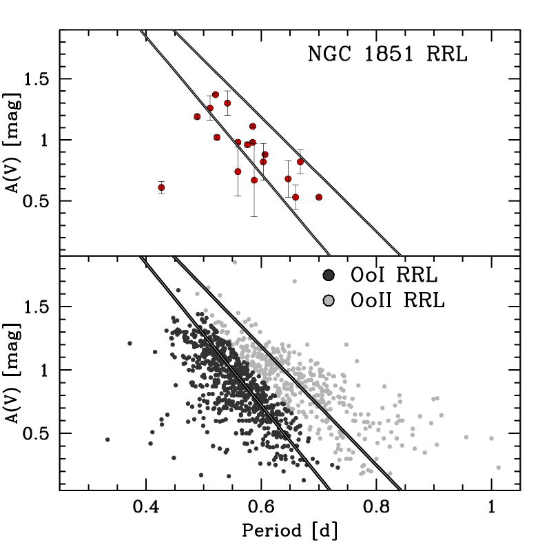
Figure 1: Top: Period-amplitude diagram for our sample of RR0 Lyrae variables in NGC 1851. Bottom: Period-amplitude relation for 1097 RR0 Lyrae variables in 40 Galactic GCs. Our division of OoI and OoII-type RR Lyrae variables are shown by dark and light circles, respectively. The lines derived by Clement & Shelton (1999) for OoI and OoII RR0 are overplotted.

In comparison, Figure 1 shows the periods and $V$-amplitudes of 1097 RR0 Lyrae variables in 40 Galactic globular clusters (Kunder et al., 2013). This sample of RR0 Lyrae variables is divided by their position in the period-amplitude plane following the lines that Clement & Shelton (1999) derived for Oosterhoff I and Oosterhoff II RR0 stars (see Figure 1). Those RR Lyrae variable falling closest to the OoI line are designated as OoI-type RR Lyrae stars, and those falling closest to the OoII line are the OoII-type variables.

We define an Oosterhoff ratio for each GC, which is simply the number of OoI-type RR0 Lyrae stars compared to the total number of RR0 Lyrae stars in the GC, $\rm OoI_{RR0}/Tot_{RR0}$. Figure 2 shows the histogram of the Oosterhoff ratio of the GCs in our sample. Our defined Oosterhoff ratio splits the Milky Way GCs into two groups; the OoI-type clusters have RR Lyrae variables with shorter periods for a given amplitude and hence have larger Oosterhoff ratios (with respect to the OoII-type clusters). Further, there is an absence of clusters falling in the “gap”. We therefore believe that our Oosterhoff ratio is useful to distinguish between OoI- and OoII-type GCs.

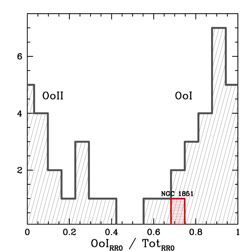
Figure 2: A histogram of the ratio of OoI stars in the Milky Way GCs. The Oosterhoff ratio of the NGC 1851 RR0 Lyrae stars is highlighted.

3 Synthetic HB Modeling

Our synthetic HB calculations are carried out to provide a simple and attractive explanation for the cluster HB and IS morphology, keeping the number of free parameters to a minimum, yet still reproducing the RR Lyrae properties that make this cluster stand out as having an unusual Oosterhoff type. The HB evolutionary tracks used are from the BaSTI stellar library (Pietrinferni et al., 2004, 2006, 2009). The horizontal part of the HB, which includes the RR Lyrae instability strip, makes up $\sim$10% of the cluster stellar sample brighter than $V$ = 21 mag; this is the component our study focuses on modelling. To be considered a match to the observations, the synthetic HB model must agree with four specific observational constraints. The first is that the number ratio of the progeny of the SGBb to the progeny of the SGBf subpopulations has to satisfy the 70:30 ratio observed along the SGB (Milone et al., 2009). The second is that the $\rm(B\thinspace{:}V\thinspace{:}R)$ (blue :variable :red HB) ratio agrees with the observed $\rm(B\thinspace{:}V\thinspace{:}R)$ = $\rm(33\pm 8\thinspace{:}10\pm 5\thinspace{:}56\pm 11)$ (in line with the results by Catelan et al., 1998; Saviane et al., 1998). The third requirement is that the theoretical periods and amplitudes agree with those observed, and the fourth that the frequency of first-overtone RR Lyrae stars (RR1) to RR0 variables is approximately $N_{\rm 1}/N_{\rm tot}$ $\sim$ 0.35 (Walker, 1998; Downes et al., 2004).

The four HB components described by Gratton et al. (2012) are used as a starting points for our calculations. As in Gratton et al. (2012), The only parameter we vary is the initial He abundance of the HB progenitors, keeping the same total RGB mass loss for all components. That the mass loss is the same for all components is not something we can prove, and we stress that this is our working assumption, and our results follow from that.

Objects from our synthetic HB that fall within the observed IS from Walker (1998) are considered RR Lyrae variables. Gratton et al. (2012) model the horizontal part of the HB component with a constant He abundance $Y$=0.265. We find a much better fit to the RR Lyrae properties, however, by assuming a continuous He distribution between $Y$=0.248 and 0.280 (see Figure 3). In our simulation, the mean He abundance in the IS is $<Y>$=0.271, close to the constant abundance $Y$=0.265 employed by Gratton et al. (2012) for this component, and the mean mass is ${\rm<M>}$ = $\rm 0.634~{}M_{\sun}$.

Figure 3 shows the periods of the RR Lyrae variables in our simulation as compared to the observed periods, where the theoretical periods are calculated for all HB stars falling within the observed IS using the Di Criscienzo et al. (2004) RR Lyrae pulsation models. The RR1 variables are fundamentalized via log $\rm P_{0}\sim logP+0.127$, where $\rm P_{0}$ is the fundamental mode period. A Kolmogorov-Smirnov (KS) test between the observed periods and the synthetic RR Lyrae periods returns a probability P=0.86, well above the default threshold ${\rm P_{th}}$=0.05 below which one rejects the null hypothesis. On this basis, we find that the synthetic periods from our simulated HB and the observed periods agree well with each other.

The ratio of first overtone to total RR Lyrae variables in our simulation is $N_{\rm 1}/N_{\rm tot}$ $\sim$0.30, in agreement with that observed. In contrast, simulations using a constant helium for the portion of the HB containing the IS (as in Gratton et al., 2012) do not fit the constraints given by the NGC 1851 RR Lyrae variables as well. For example, adopting $Y$=0.265 results in an $\rm N_{1}/N_{tot}$ = 0.11 (versus the observed $\rm N_{1}/N_{tot}$ = 0.28).

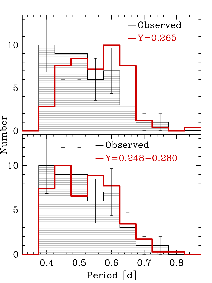
Figure 3: Top: A comparison between the observed NGC 1851 RR Lyrae periods versus the theoretical periods with a constant Y=0.265 (Gratton et al. 2012). Bottom: The results when using a He abundance with minor helium variations ($Y$$\sim$0.248-0.280) versus the observed periods.

4 Conclusions

Modern theoretical synthetic HB models are used to investigate the RR Lyrae properties of NGC 1851. Both the RR Lyrae period distribution and the number ratio of first overtone RR Lyrae to total RR Lyrae stars, $\rm N_{1}/N_{tot}$, provide constraints pertaining to the component of the HB containing the IS. It is straightforward to reproduce the observed distribution of RR Lyrae stars inside the instability strip with minor He variations ($Y$$\sim$0.248-0.280).

In general, the RR Lyrae variables with $Y$ $<$ 0.27 fall in the OoI area of the PA diagram, whereas the RR Lyrae variables with $Y$ $>$ 0.27 fall close to the OoII line. Assuming that the period-amplitude diagram can be effectively used to classify RR Lyrae stars into an Oosterhoff type, this means that He and Oosterhoff type are correlated in this cluster. This is not completely unexpected, as an increase in He makes RR Lyrae variables brighter and, as a consequence, higher helium abundance makes their pulsational period longer at fixed temperature/color (Bono et al., 1997).

References

- Bono et al. (1997) Bono, G., Caputo, V., Castellani, V., & Marconi, M. 1997, A&AS, 121, 327
- Cassisi et al. (2008) Cassisi, S., Salaris, M., Pietrinferni, A., Piotto, G., Milone, A. P., Bedin, L. R., & Anderson, J. 2008, ApJ, 672, L115
- Catelan et al. (1998) Catelan, M., Borissova, J., Sweigart, A. V., & Spassova, N. 1998, ApJ, 494, 265
- Clement & Shelton (1999) Clement, C.M. & Shelton, I. 1999, ApJ, 515, 88
- Di Criscienzo et al. (2004) Di Criscienzo, M., Marconi, M., & Caputo, F. 2004, ApJ, 612, 1092
- Dotter et al. (2010) Dotter, A., Sarajedini, A., Anderson, J. et al. ApJ, 708, 698
- Downes et al. (2004) Downes, R.A., Margon, B., Homer, L. & Anderson, S.F. 2004, AJ, 128, 2288
- Gratton et al. (2010) Gratton, R.G., Carretta, E., Bragaglia, A., Lucatello, S., D Orazi, V. 2010, A&A, 517, 81
- Gratton et al. (2012) Gratton, R.G. et al. 2012, A&A, 539, 19
- Grundahl et al. (1999) Grundahl, F., Catelan, M., Landsman, W. B., Stetson, P. B., & Andersen, M. I. 1999, ApJ, 524, 242
- Han et al. (2009) Han, S.-I., Lee, Y.-W., & Joo, S.-J. et al. 2009, ApJ, 707, L190
- Kunder et al. (2013) Kunder, A.M., Salaris, M., Cassisi, S. et al. 2013, AJ, 145, 25
- Milone et al. (2008) Milone, A. P., et al. 2008, ApJ, 673, 241
- Milone et al. (2009) Milone, A. P., et al. 2009, A&A 503, 755
- Pietrinferni et al. (2004) Pietrinferni, A., Cassisi, S., Salaris, M., & Castelli, F. 2004, ApJ, 612, 168
- Pietrinferni et al. (2006) Pietrinferni, A., Cassisi, S., Salaris, M., & Castelli, F. 2006, ApJ, 642, 797
- Pietrinferni et al. (2009) Pietrinferni , A., Cassisi, S., Salaris, M., Percival, S. & Ferguson, J. W. 2009 ApJ, 697, 275
- Salaris et al. (2008) Salaris, M., Cassisi, S., & Pietrinferni, A. 2008, ApJL, 678, L25
- Saviane et al. (1998) Saviane, I., Piotto, G., Fagotto, F., Zaggia, S., Capaccioli, M., & Aparicio, A. 1998, A&A, 333, 479
- Sumerel et al. (2004) Sumerel, A.N., Corwin, T. M., Catelan, M., Borissova, J., Smith, H. A. 2004, IBVS 5533
- Ventura et al. (2009) Ventura, P., Caloi, V., D’Antona, F., Ferguson, J., Milone, A., & Piotto, G.P. 2009, MNRAS, 399, 934
- Walker (1998) Walker, A.R. 1998, AJ, 116, 220