Asymptotic behavior of a scalar field with an arbitrary potential trapped on a Randall-Sundrum’s braneworld: the effect of a negative dark radiation term on a Bianchi I brane

Abstract

In this work we present a phase space analysis of a quintessence field and a perfect fluid trapped in a Randall- Sundrum’s Braneworld of type 2. We consider a homogeneous but anisotropic Bianchi I brane geometry. Moreover, we consider the effect of the projection of the fivedimensional Weyl tensor onto the three-brane in the form of a negative Dark Radiation term. For the treatment of the potential we use the “Method of $f$-devisers” that allows investigating arbitrary potentials in a phase space. We present general conditions on the potential in order to obtain the stability of standard 4D and non-standard 5D de Sitter solutions, and we provide the stability conditions for both scalar field-matter scaling solutions, scalar field-dark radiation solutions and scalar field-dominated solutions. We find that the shear-dominated solutions are unstable (particularly, contracting shear-dominated solutions are of saddle type). As a main difference with our previous work, the traditionally ever-expanding models could potentially re-collapse due to the negativity of the dark radiation. Additionally, our system admits a large class of static solutions that are of saddle type. These kinds of solutions are important at intermediate stages in the evolution of the universe, since they allow the transition from contracting to expanding models and viceversa. New features of our scenario are the existence of a bounce and a turnaround, which lead to cyclic behavior, that are not allowed in Bianchi I branes with positive dark radiation term. Finally, as specific examples we consider the potentials $V\propto\sinh^{-\alpha}(\beta\phi)$ and $V\propto\left[\cosh\left(\xi\phi\right)-1\right]$ which have simple $f$-devisers.

I Introduction

The idea that our Universe is a brane embedded in a 5–dimensional space, on which the particles of the standard model are confined, while gravity is allowed to propagate not only on the brane but also in the bulk of the higher-dimensional manifold, was proposed by Randall and Sundrum (1999a); Randall and Sundrum (1999b). These braneworld models were baptized as Randall-Sundrum type $1$ (RS1) and type $2$ (RS2). The original motivation of Randall and Sundrum (1999a) to propose the RS1 scenario was to look for an explanation to the hierarchy problem, whereas the motivation of the RS2 scenario was to propose an alternative mechanism to the Kaluza-Klein compactifications (Randall and Sundrum, 1999b).

It is well-known that the cosmological field equations on the RS2 brane are essentially different from the standard 4–dimensional cosmology (Binetruy et al., 2000a, b; Bowcock et al., 2000; Apostolopoulos et al., 2005). In fact, in the case of a flat Friedmann-Robertson-Walker metric (FRW) the Friedmann equation is modified by:

$$H^{2}=\frac{1}{3}\kappa^{2}\rho\left(1+\frac{\rho}{2\lambda}\right),$$ (1)

where $\lambda>0$ is the brane tension. These models also have an appreciable cosmological impact in the inflationary scenario (Hawkins and Lidsey, 2001; Huey and Lidsey, 2001, 2002). However, is not the study of brane inflation the purpose of the present paper, but the investigation of the bouncing behavior, the study of the asymptotic structure of the model and, also, the investigation of the role of static solutions in the cosmic evolution.

The dynamics of RS2 branes has been widely investigated using the dynamical systems approach (Szydlowski et al., 2002; van den Hoogen et al., 2003; van den Hoogen and Ibanez, 2003; Toporensky et al., 2003; Savchenko and Toporensky, 2003; Solomons et al., 2006; Haghani et al., 2012). In (Campos and Sopuerta, 2001a) was studied the asymptotic behavior of FRW, Bianchi I and V brane in the presence of perfect fluid. The same authors analyzed the contribution of the non-vanishing (positive and negative) dark radiation term, $\cal U$, in the dynamics of FRW and Bianchi I branes in (Campos and Sopuerta, 2001b). Goheer and Dunsby (2002, 2003) extended the previous study by the inclusion of a scalar field with an exponential potential in FRW and Bianchi I branes. In the first case the authors discussed the changes of the phase space compared with the general relativistic case (Goheer and Dunsby, 2002) while for the Bianchi I brane, the effects of considering a non vanishing projection of the Weyl tensor on the brane were studied taking into account four different scenarios: a) ${\cal U}\geq 0$, ${}^{3}R\leq 0$; b) ${\cal U}\geq 0$, ${}^{3}R\geq 0$; c) ${\cal U}\leq 0$, ${}^{3}R\leq 0$; d) ${\cal U}\leq 0$, ${}^{3}R\geq 0$ (Goheer and Dunsby, 2003). These studies were extended to the case of a scalar field with an arbitrary potential trapped in FRW branes by Leyva et al. (2009); Escobar et al. (2012a), while the impact of a positive dark radiation term (${\cal U}\geq 0$) on the dynamics of a Bianchi I brane, supported by a scalar field with an arbitrary potential, was investigated by Escobar et al. (2012b).

The term $\cal U$ represents the scalar component of the electric (Coulomb) part of the 5-dimensional Weyl tensor of the bulk (Shiromizu et al., 2000; Sasaki et al., 2000). $\cal U$ scales just like radiation with a constant $\mu$, i.e., ${\cal U}=\mu a^{-4}$, for that reason it is called the dark radiation. The coefficient $\mu$ is a constant of integration obtained by integrating the 5-dimensional Einstein equations (Binetruy et al., 2000a, b; Langlois et al., 2001; Barrow and Maartens, 2002; Kraus, 1999; Hebecker and March-Russell, 2001; Ida, 2000; Vollick, 2001). In FRW brane model, $\mu$ is related with the mass of the black hole in the bulk therefore $\cal U$ is positive defined (Mukohyama et al., 2000; Maartens and Koyama, 2010; Clifton et al., 2012). For anisotropic models (for instance, Bianchi I models) both positive and negative $\mu$ are possible (Campos and Sopuerta, 2001b; Goheer and Dunsby, 2003; Santos et al., 2001). Its magnitude and sign can depend on the choice of initial conditions when solving the 5-dimensional Einstein equation. Hence, even the sign of $\mu$ remains an open question (Sasaki et al., 2000; Mukohyama et al., 2000).

Dark radiation should strongly affect both big-bang nucleosynthesis (BBN) and the cosmic microwave background (CMB). Such observations can be used to constrain both the magnitude and sign of the dark radiation as well as other radiation sources (see the works by Malaney and Mathews (1993); Olive et al. (2000), and by Ichiki et al. (2002); Apostolopoulos and Tetradis (2006); Dutta et al. (2009); Diamanti et al. (2012); Gonzalez-Garcia et al. (2013)). The dark radiation restrictions for FRW brane were found in (Ichiki et al., 2002; Bratt et al., 2002). In (Ichiki et al., 2002), the constraints on BBN alone allow for $-1.23\leq\rho_{DR}/\rho_{\gamma}\leq 0.11$ in a dark radiation component, where $\rho_{\gamma}$ is the total energy density in background photons just before the BBN epoch at $T=1MeV,$ $\rho_{DR}={6{\cal U}}/{\lambda},$ and $\lambda$ is the tension of the brane. In order to compute the theoretical prediction of CMB anisotropies exactly, one must eventually solve the perturbations including the contribution from the bulk. However, in (Ichiki et al., 2002) the CMB power spectrum was used to constrain the dominant expansion-rate effect of the dark-radiation term in the generalized Friedmann equation. If the constraint from effects of dark radiation on the expansion rate are included, the allowed concordance range of dark radiation content reduces to $-0.41\leq\rho_{DR}/\rho_{\gamma}\leq 0.105$ at the 95% confidence level. Similar result was derived by Bratt et al. (2002), for high values of the 5-dimensional Planck mass, as $-1<\rho_{DR}/\rho_{\nu}<0.5$, where $\rho_{\nu}$ is the energy density contributed by a single, two-component massless neutrino.

The presence of dark radiation is associated with new degrees of freedom in the relativistic components of our Universe. Indeed, any process able to produce extra (dark) radiation produces the same effects on the background expansion of additional neutrinos, therefore, a larger value for effective number of relativistic degrees of freedom ($N_{eff}$) is obtained (Archidiacono et al., 2011). These bounds has been improved in the latest analysis by the Wilkinson Microwave Anisotropy Probe (WMAP) (Bennett et al., 2012), the South Pole Telescope (SPT) (Hou et al., 2012), the Atacama Cosmology Telescope (ACT) (Sievers et al., 2013) and Planck (Ade et al., 2013a). The main results on the effective number of neutrino species are the following:

• $N_{eff}=2.79\pm 0.56$ joint result of WMAP 7 $+$ ACT (Sievers et al., 2013),

• $N_{eff}=3.50\pm 0.42$ joint result of WMAP 7 $+$ ACT $+$ BAO $+$ HST,

• $N_{eff}=2.85^{+0.95}_{-0.91}$ joint result of WMAP 9 $+$ ACT (Di Valentino et al., 2013a), (Sievers et al., 2013),

• $N_{eff}=3.23^{+0.77}_{-0.76}$ joint result of WMAP 9 $+$ ACT $+$ BAO $+$ HST (Di Valentino et al., 2013a),

• $N_{eff}=3.71\pm 0.35$ joint result of WMAP 7 $+$ South Pole Telescope (SPT)$+$ BAO $+$HST (Hou et al., 2012),

• $N_{eff}=3.84\pm 0.40$ joint result of WMAP 9$+$ eCMB $+$ BAO $+$ HST (Hinshaw et al., 2012),

and more recently

• $N_{eff}=3.83\pm 0.54$ at $95\%$ confidence level from joint result of Planck satellite $+$ HST (Ade et al., 2013a) and

• $N_{eff}=3.62^{+0.50}_{-0.48}$ at $95\%$ confidence level from joint result of Planck satellite $+$ HST $+$ ACT $+$ SPT $+$WMAP 9 (Ade et al., 2013a).

These latter bounds indicate the presence of an extra dark radiation component at the $\approx 2\sigma$ confidence level (Di Valentino et al., 2013b) and the existence of a tension between the latest ACT and SPT results. So the presence of a dark radiation source, like sterile neutrinos from the ($3+2$) or ($3+3$) models (Di Valentino et al., 2013b), or a (negative) source of dark radiation with an geometrical origin like in our case are not ruled out by observations.

In the other hand, observation of the CMB tell us that our Universe is isotropic a great accuracy, to within a part in $10^{5}$ (Hinshaw et al., 2007; Komatsu et al., 2011). The natural framework to approach this highly isotropic Universe we observe today, is to assume that the Universe started in a highly initial anisotropic state and then, a dynamical mechanism get rid of almost all its anisotropy. Several candidates have been proposed to explaining this behavior, among them, inflation mechanisms (Guth, 1981; Linde, 1982) is the most popular. In these line, the simplest generalization of a FRW cosmologies are Bianchi cosmologies, the latter provide anisotropic but homogeneous cosmologies (Misner et al., 1974), where the central point of discussion is if the Universe can isotropize without fine-tuning the parameters of the model. The isotropization of Bianchi I braneworld cosmologies has been investigated, from several points of view, in the literature (Maartens et al., 2001; Niz et al., 2008; Goheer and Dunsby, 2003; Toporensky and Tretyakov, 2005). In (Maartens et al., 2001), is shown that large anisotropy does not negatively affect inflation in a Bianchi I braneworld; also it is shown that the initial expansion of the universe is quasi-isotropic if the scalar field possesses a large kinetic term. While considering negative values of dark radiation (${\cal U}<0$) in Bianchi I models lead to very interesting solutions for which the universe can both collapse or isotropize (Campos and Sopuerta, 2001b, a; Goheer and Dunsby, 2002, 2003; Toporensky and Tretyakov, 2005). More recently, the Planck results (Ade et al., 2013a, b) are rekindled a renewed interest in these Bianchi cosmologies since some anisotropic anomalies seem to appear. At the same time, is required that this isotropization is accompanied with a phase of accelerated expansion in order to be a good candidate to explain the strong results that indicates the current speeding up of the observable universe (Riess et al., 1998; Perlmutter et al., 1999). This latter observational fact is approached from two directions: modifying the gravitational sector (Clifton et al., 2012) or introducing an hypothetical form of energy baptized as Dark Energy (Copeland et al., 2006). From this viewpoint, a model in which a dark energy component lives in a Bianchi braneworld combines both approaches. All the above reasons motivate the investigation of a homogeneous but anisotropic brane model with ${\cal U}<0.$

In this paper, we study the dynamics of a scalar field with an arbitrary potential trapped in a RS-2 brane-world model. We consider a homogeneous but aniso–tropic Bianchi I (BI) brane filled also with a perfect fluid. Furthermore, we consider the effect of the projection of the five-dimensional Weyl tensor onto the three-brane in the form of a negative dark radiation term. The results presented here complement our previous investigation (Escobar et al., 2012b) where we considered the effect of a positive dark radiation term on the brane.

For the treatment of the potential we use a modification of the method introduced for the investigation of scalar fields in isotropic (FRW) scenarios (Fang et al., 2009; Matos et al., 2009; Leyva et al., 2009; Urena-Lopez, 2012; Copeland et al., 2009; Dutta et al., 2009), and that has been generalized to several cosmological contexts in (Escobar et al., 2012a, b; Farajollahi et al., 2011; Xiao and Zhu, 2011). The modified method, that we call “Method of $f$-devisers”, allows us to perform a phase-space analysis of a cosmological model, without the need for specifying the potential. This is a significant advantage, since one can first perform the analysis for arbitrary potentials and then just substitute the desired forms, instead of repeating the whole procedure for every distinct potential. This investigation represents a further step in a series of works devoted to the use of the general procedure of $f$-devisers for investigating both FRW and Bianchi I branes, initiated in our previous works (Escobar et al., 2012a, b).

A main difference with our results in (Escobar et al., 2012b), is that the traditionally ever-expanding models could potentially recollapse due to the negativity of the dark radiation (${\cal U}<0$). New features of our scenario are the possibility of a bounce and a turnaround, which leads to cyclic behavior. This behavior is not allowed in Bianchi I branes with positive dark radiation term (Escobar et al., 2012b). Observe that in the usual Randall-Sundrum scenario the tension of the brane is positive. In this case, $H=0$ if and only if the total matter density satisfy $\rho=0.$ For this reason the bounce is not possible for the usual braneworld scenario (flat geometry, positive brane tension). However, it is possible to have a bounce provided the existence of a negative correction (in our context, the negative “dark radiation” component) to the Friedman equation (1) compensating the new positive contribution $\frac{\kappa^{2}\rho^{2}}{6\lambda}$ (due to presence of the brane on the higher dimensional bulk space), still having a total non-negative r.h.s.

Also, our system admits a large class of static solutions that are of saddle type. This kind of solutions are important at intermediate stages in the evolution of the universe since they allow the transition from expanding to contracting models, and viceversa. The interest in static solutions in the cosmological setting goes back to the discovering of Einstein static (ES) model. This model was proposed by Einstein (1917) as an attempt to incorporate Mach’s principle into the general relativity (GR) and also to overcome the boundary conditions of the theory. Several issues of this model have been intensively investigated. Eddington (1930); Harrison (1967); Gibbons (1987), considered inhomogeneous and anisotropic perturbations to ES model; the stability issue for ghost massless scalar field cosmologies was studied by Barrow and Tsagas (2009); the case for $f(R)$ theories was studied by Goswami et al. (2008); Goheer et al. (2009), where ES solutions can provide the link between decelerating/accelerating phases in these theories in the same way as in GR (Barrow et al., 2003). The stability analysis of the ES universe, and other kinds of static solutions in the context of brane cosmology with dust matter and anisotropic geometry was presented by Campos and Sopuerta (2001b, a). Here we present several classes of static solutions for a Bianchi I brane containing a scalar field with an arbitrary potential. This class of solutions are more general than the presented by Campos and Sopuerta (2001b, a); Goheer and Dunsby (2003).

The main objectives of our investigation are:

• To analyze the bouncing and cyclic behavior of some cosmological solutions in our set up.

• To obtain qualitative information about the past and future asymptotic structure of our model, without the need to repeat the whole procedure each time the scalar field potential is chosen. Especially, we want to obtain general conditions for late-time isotropization. The method of $f$-devisers is the key for this point.

• To investigate the viability of static solutions as the link between contracting and expanding solutions in our set up.

• To generalized previous results obtained by us and by other authors that were discussed in the literature.

The paper is organized as follows. In section II we present our general approach for the investigation of arbitrary potentials. In section III are presented the cosmological equations of our model. In section V we proceed to the dynamical system analysis of the cosmological model under consideration. For this purpose we use the method of $f$- devisers discussed in section II, and we introduce local charts adapted to each of the more interesting singular points. In this way, we analyze the stability of the shear-dominated solutions, the stability of the de Sitter solutions and the stability of the solutions with 5D corrections. In section VI we summarize our analytical results and proceed to the physical discussion specially to the comparison with previous results. Particular emphasis is made on static solutions. In section VII we illustrate our analytical results for two examples: the cosh-like potential $V(\phi)=V_{0}\left[\cosh\left(\xi\phi\right)-1\right]$ (Ratra and Peebles, 1988; Wetterich, 1988; Matos and Urena-Lopez, 2000; Sahni and Wang, 2000; Sahni and Starobinsky, 2000; Lidsey et al., 2002; Pavluchenko, 2003; Matos et al., 2009; Copeland et al., 2009; Leyva et al., 2009) and the inverted sinh-like potential $V(\phi)=V_{0}\sinh^{-\alpha}(\beta\phi)$ studied by Ratra and Peebles (1988); Wetterich (1988); Urena-Lopez and Matos (2000); Sahni and Starobinsky (2000); Pavluchenko (2003); Copeland et al. (2009); Leyva et al. (2009) which have simple $f$-devisers. Is worthy to mention that this procedure is general and applies to other potentials different from the cosh-like, the inverted sinh-like and the exponential one. Finally, in section VIII are drawn our general conclusions.

II “Method of $f$-devisers”

Table 1: Explicit form of the $f(s)$-function for some quintessence potentials.

Potential	$f(s)$
$V(\phi)=V_{0}\left[\cosh\left(\xi\phi\right)-1\right]$	$-\frac{1}{2}(s^{2}-\xi^{2})$
$V(\phi)=V_{0}\sinh^{-\alpha}(\beta\phi)$	$\frac{s^{2}}{\alpha}-\alpha\beta^{2}$
$V(\phi)=V_{0}e^{-\lambda\phi}+\Lambda$	$-s(s-\lambda)$
$V(\phi)=V_{0}\left[e^{\alpha\phi}+e^{\beta\phi}\right]$	$-(s+\alpha)(s+\beta)$

In this section we present a general method, called “Method of $f$-devisers”, that allows us to perform a phase-space analysis of a cosmological model, without the need for specifying the potential. This procedure consist of a modification of a method used in isotropic (FRW) scalar field cosmologies for the treatment of the potential of the scalar field (Fang et al., 2009; Matos et al., 2009; Leyva et al., 2009; Urena-Lopez, 2012; Copeland et al., 2009), that has been generalized to several cosmological contexts by Farajollahi et al. (2011); Xiao and Zhu (2011); Escobar et al. (2012a, b). An earlier attempt to introduce the “Method of $f$-devisers” as in the present form was by Matos et al. (2009) in the context of FRW cosmologies. However, there the authors restricted their attention to a scalar field dark-matter model with a cosh-like potential, and there was revealed that the late-time attractor is always the de Sitter solution. In section VII we will take this potential as an example of the application of the present method in the context of brane cosmology.

The procedure for deriving the “Method of $f$-devisers” is as follows. Let us define the two dynamical variables

$$s = -\frac{V^{\prime}(\phi)}{V(\phi)}\,,$$ (2)

$$f = \frac{V^{\prime\prime}(\phi)}{V(\phi)}-\frac{V^{\prime}(\phi)^{2}}{V(\phi)^{2}},$$ (3)

while keeping the potential still arbitrary.

In the formulas (2) and (3), the primes denote differentiation with respect to $\phi$.

Now, for the usual ansatzes of the cosmological literature, it results that $f$ can be expressed as an explicit one-valued function of $s$, that is $f=f(s)$ (as can be seen in table 1), and therefore we obtain a closed dynamical system for $s$ and a set of normalized-variables. So, instead to consider a fixed potential $V,$ from the beginning, we examine the asymptotic properties of our cosmological model, by considering suitable (general) conditions on an arbitrary input function

$$f:\mathbb{R}\rightarrow\mathbb{R},\;\;s\rightarrow f(s).$$

Now, once we have considered a function $f$ as an input, we can solve the equation

$$\frac{V^{\prime\prime}(\phi)}{V(\phi)}-\frac{V^{\prime}(\phi)^{2}}{V(\phi)^{2}}=f\left(-\frac{V^{\prime}(\phi)}{V(\phi)}\right),$$ (4)

that gives the solution $V(\phi)$ up to two arbitrary constants, provided $f$ is smooth enough such that the Initial Value Problem associated to (4) is well-posed. In other words, it is possible to reconstruct the corresponding potential from a given $f(s)$.

The ODE (4) is equivalent to the system

$$\frac{ds}{d\phi}=-f(s),$$ (5)

$$\frac{dV}{d\phi}=-sV.$$ (6)

From this system are deduced the quadratures

$$\phi(s) = \phi_{0}-\int_{s_{0}}^{s}\frac{1}{f(K)}\,dK,$$ (7)

$$V(s) = e^{\int_{s_{0}}^{s}\frac{K}{f(K)}\,dK}\bar{V}_{0},$$ (8)

where the integration constants satisfies $V(s_{0})=\bar{V}_{0}$, $\phi(s_{0})=\phi_{0}$. The relations (7) and (8) are always valid and they provide the potential in an implicit form. The integrability conditions for (7) and (8) impose additional constraints to $f$. For the usual cosmological cases of table 1 the potential can be written explicitly, that is $V=V(\phi)$, after elimination of $s$ between (7) and (8).

The direct derivation of the function $f(s)$ from a given $V(\phi)$, as well as the reconstruction procedure for obtaining $V(\phi)$ from a given $f$-function is what we call “Method of $f$-devisers”. In the section V we use this method for investigating the phase portrait of quintessence fields trapped in a Randall-Sundrum Braneworld in the case of an anisotropic Bianchi I brane with a negative dark radiation term.

The method, as introduced here, has the significant advantage that one can first perform the analysis for arbitrary potentials, by considering general mathematical conditions about $f(s),$ and then just substituting the desired forms, instead of repeating the whole procedure for every given potential. More importantly is that the method does not depend on the cosmological scenario, since it is constructed on the scalar field and its self-interacting potential, and can be generalized to several scalar fields (for example to quintom models (Leon et al., 2012)). The disadvantages are that such a generalization is only possible if in the model do not appear functions that contains mixed terms of several scalar fields. For example, cosmological models containing an interaction term given by $V(\phi,\varphi)$ discussed by Lazkoz and Leon (2006) and by Lazkoz et al. (2007), where $\phi,\varphi$ are the scalar fields, cannot be investigated using the method of $f$-devisers. On the other hand, in the single field case the method cannot be applied if the model contains more than one “arbitrary” function depending on the scalar field, as for example a cosmological model containing a potential $V(\phi)$ and coupling function $\chi(\phi)$, studied in the context of non-minimally coupled scalar field cosmologies by Leon (2009); Leon et al. (2010); Leon and Fadragas (2012). In such a case the more convenient approach is to consider the scalar field itself as a dynamical variable.

III The model

In this paper we follow (Campos and Sopuerta, 2001b; Goheer and Dunsby, 2003) where is given a brief outline of the considerations that lead to the effective Einstein equations for Bianchi I models. The metric in the brane is given by $ds^{2}=-a_{0}^{2}(t)dt^{2}+\sum a_{i}(t)(dx^{i})^{2}.$

The set up is as follows. Using the Gauss-Codacci equations, relating the four and five-dimensional spacetimes, we obtain the modified Einstein equations on the brane (Shiromizu et al., 2000; Sasaki et al., 2000):

$$G_{ab}=-\Lambda_{4}g_{ab}+\kappa^{2}T_{ab}+\kappa_{(5)}^{4}S_{ab}-{\cal E}_{ab},$$ (9)

where $g_{ab}$ is the four-dimensional metric on the brane and $G_{ab}$ is the Einstein tensor, $\kappa$ is the four-dimensional gravitational constant, and $\Lambda_{4}$ is the cosmological constant induced in the brane. $S_{ab}$ are quadratic corrections in the matter variables. Finally, the tensor ${\cal E}_{ab}$ is a correction to the field equations on the brane coming from the extra dimension. This tensor is responsible for the so-called Dark Radiation, this fact will be more evident in the following developments.

More precisely, ${\cal E}_{ab}$ are the components of the electric part of the 5D Weyl tensor of the bulk projected on the brane (see (Shiromizu et al., 2000) and the review by Maartens and Koyama (2010) for more details). Following (Goheer and Dunsby, 2003; Campos and Sopuerta, 2001b; Maartens, 2000), from the energy-momentum tensor conservation equations ($\nabla_{a}T^{a}_{b}=0$) and equations (9) we get a constraint on $S_{ab}$ and ${\cal E}_{ab}$:

$$\nabla^{a}\left({\cal E}_{ab}-\kappa_{(5)}^{4}S_{ab}\right)=0.$$ (10)

In general we can decompose ${\cal E}_{ab}$ with respect to a chosen 4-velocity field $u^{a}$(Maartens, 2000) as:

$${\cal E}_{ab}=-\left(\frac{\kappa_{(5)}}{\kappa}\right)^{4}\left[{\cal U}\left(u_{a}u_{b}+\frac{1}{3}h_{ab}\right)+{\cal P}_{ab}+2u_{(a}{\cal Q}_{b)}\right],$$ (11)

where

$${\cal P}_{(ab)}={\cal P}_{ab},\;\;\;{\cal P}^{a}_{a}=0,\;\;\;{\cal P}_{ab}u^{b}=0,\;\;\;{\cal Q}_{a}u^{a}=0,$$ (12)

and here the scalar component ${\cal U}$ is referred as the “dark radiation” energy density due to it has the same form as the energy-momentum tensor of a radiation perfect fluid. ${\cal Q}_{a}$ is an spatial vector that corresponds to an effective nonlocal energy flux on the brane and ${\cal P}_{ab}$ is an spatial, symmetry and trace-free tensor which is an effective non local anisotropic stress. Another important point is that the $9$ independent component in the trace-free ${\cal E}_{ab}$ are reduced to $5$ degrees of freedom by equation (10) (Maartens and Koyama, 2010), i.e., the constraint equation (10) provides evolution equations for ${\cal U}$ and ${\cal Q}_{a}$, but not for ${\cal P}_{ab}$.

Taking into account the effective Einstein’s equations (9), the consequence of having a Bianchi I model on the brane is (Maartens et al., 2001)

$${\cal Q}_{a}=0.$$ (13)

Since we have no information about the dynamics of the tensor ${\cal P}_{ab}$ we assume (Campos and Sopuerta, 2001b; Goheer and Dunsby, 2003):

$${\cal P}_{ab}=0,$$ (14)

this condition, together with (13) and (10), implies:

$$D_{a}{\cal U}=0\Leftrightarrow{\cal U}={\cal U}(t).$$ (15)

Using the above conditions over ${\cal Q}_{a}$ and ${\cal P}_{ab}$ (13)-(14), setting the effective cosmological constant in the brane to zero, i.e., $\Lambda_{4}=0$ , the effective Einstein equations (9) for Bianchi I models (which have zero 3-curvature, i.e., $R^{(3)}=0$) become:

$$H^{2}=\frac{1}{3}\rho_{T}\left(1+\frac{\rho_{T}}{2\lambda}\right)+\frac{1}{3}\sigma^{2}+\frac{2{\cal U}}{\lambda},$$ (16)

$$\dot{H}=-\frac{1}{2}\left(1+\frac{\rho_{T}}{\lambda}\right)\left(\dot{\phi}^{2}+\gamma\rho_{m}\right)-\frac{4{\cal U}}{\lambda}-\sigma^{2},$$ (17)

$$\dot{\sigma}=-3H\sigma,$$ (18)

$$\dot{\rho}_{m}+3H(\rho_{m}+p_{m})=0,$$ (19)

$$\ddot{\phi}+3H\dot{\phi}+\partial_{\phi}V=0,$$ (20)

where $H$ is the Hubble factor, $\rho_{m}$ is the matter energy density, $\phi$ is an scalar field with self-interacting positive potential $V(\phi)$. It is convenient to relate the pressure of the background matter $p_{m}$ and its energy density $\rho_{m}$ by

$$p_{m}=(\gamma-1)\rho_{m}.$$ (21)

The parameter $\gamma$ is a constant parameter which is just the barotropic index of the background matter density $\rho_{m}.$ $\sigma$ is a measure of the brane anisotropies and $\cal{U}$ denotes the dark radiation term. Finally, $\rho_{T}$ in the equation (16) denotes the total energy density on the brane (with tension $\lambda>0$), and is given by ${\rho_{T}}=\frac{1}{2}\dot{\phi}^{2}+V(\phi)+\rho_{m},$ and it is positive definite. That is, we considered an scalar field density and a background matter density as our Universe (brane) content, and we have neglected the radiation in the total matter (that we recall is confined to the brane). We have used units in which $\kappa^{2}=8\pi G=1.$

The dark radiation term in (16)-(17) evolves as ${\cal U}(t)=\frac{\mu}{a(t)^{4}},$ where $\mu$ is a constant parameter (Maartens, 2000). From the brane base formalism, $\mu$ is just an integration constant that can take any sign (which actually could be negative, zero or positive, as we will discuss next). However it was shown, from the bulk based formalism, that for all possible homogeneous and isotropic solutions on the brane, the bulk spacetime should be Schwarzschild-AdS. In this case, it is possible to identify $\mu$ with the mass of a black hole in the bulk ($m=\frac{2\mu}{\lambda}$). From this fact, $\mu$ should be positive (Mukohyama et al., 2000; Maartens and Koyama, 2010; Clifton et al., 2012). However, for anisotropic models such identification of $\mu$ with a mass-term is not possible, i.e., $\mu$, and therefore ${\cal U}$, can take any sign (Campos and Sopuerta, 2001b; Santos et al., 2001; Goheer and Dunsby, 2003). As shown in Eq. (16), dark radiation is strictly a correction to the Friedmann equation that scale as radiation, but its origin is geometric and it has no interaction (e.g., Compton scattering) with other matter fluids. The total radiation (including photons and neutrinos) that is confined to the brane (which represents the universe) should be positive. However, it is possible to obtain relevant cosmological results if we allows for the existence of, even a very tiny, negative dark radiation component. Interesting, for ${\cal U}<0$ the expanding phase could experience the cosmological turnaround triggered by the negativity of this dark radiation, and similarly the contracting phase can leads to a cosmological bounce and then to expansion.

IV The bounce and the turnaround

Before proceeding to the detailed investigation of the model (16)-(20) using dynamical systems tools, let us discuss the above system using a heuristic reasoning. Integrating equation (18) and (19) we obtain that $\sigma=\sigma_{0}a^{-3}$ and $\rho_{m}=\rho_{m0}a^{-3\gamma},$ while as discussed in the introduction ${\cal U}=\mu a^{-4}.$ Let us examine the case of $\frac{\dot{\phi}^{2}}{2}\gg V(\phi),$ thus, $\rho_{\phi}\approx\rho_{\phi 0}a^{-6},$ which implies $\rho_{T}=\rho_{\phi 0}a^{-6}+\rho_{m0}a^{-3\gamma}.$ Then equation (16) reduces to

$$3H^{2}=\frac{\rho_{m0}^{2}a^{-6\gamma}}{2\lambda}+\frac{\rho_{m0}\rho_{\phi 0}a^{-3\gamma-6}}{\lambda}+\frac{\rho_{\phi 0}^{2}}{2\lambda}a^{-12}+$$

$$\ \ \ \ \ \ \ \ \ \ \ \ +\left(\rho_{\phi 0}+\sigma_{0}^{2}\right)a^{-6}+\rho_{m0}a^{-3\gamma}-\frac{6|\mu|}{\lambda}a^{-4}.$$ (22)

There are several cases depending of the values of $\gamma$. Suppose that the universe lies currently in the usual expanding phase, i.e. $H(a=a_{0})>0,$ where $a_{0}$ denotes the scale of the universe at the present time. We take as a reference universe’s state the present expanding one. Thus a future zero of $H$ will correspond to a turnaround, while a past one corresponds to a bounce.

• For $\gamma>4/3$ the dark radiation term in equation (IV) falls less rapidly than the matter terms, making the future turnaround inevitable for any initial negative $\cal U$.

• For $\gamma=4/3,$ the last two terms in the r.h.s. of (IV) are equally important in a low-energy regime, and the condition for the future turnaround is

  $$\rho_{m0}<6|\mu|/\lambda.$$

• For $1<\gamma<\frac{4}{3},$ the leading terms in the r.h.s. of (IV) that are equally important are the last two terms (since the terms scaling as $a^{-6}$ goes very fast to zero). As a result, we obtain that the condition $H=0$ leads to the equation:

  $$\rho_{m0}a^{4-3\gamma}-\frac{6|\mu|}{\lambda}=0.$$

  This equation has the positive root given by

  $$a_{+}=\left[\frac{6|\mu|}{\lambda\rho_{m0}}\right]^{\frac{1}{4-3\gamma}}.$$

  If $a_{+}>a_{0}$ (the scale factor today) it corresponds to the future of the Universe under consideration and indicates the point of turnaround. If $a_{+}<a_{0}$, will describe the past and corresponds to a bounce.

• For $\gamma=1,$ the leading terms in the r.h.s. of (IV) that are equally important are the first and the last three terms. As a result, we obtain that the condition $H=0$ leads to the cubic equation for the scale factor:
  

  $$a^{3}-\frac{6|\mu|}{\lambda\rho_{m0}}a^{2}+\left[\frac{\rho_{m0}}{2\lambda}+\frac{\rho_{\phi 0}}{\rho_{m0}}+\frac{\sigma_{0}^{2}}{\rho_{m0}}\right]=0.$$

  Applying Descartes’s rule, this equation has always one negative root and two real positive or either complex conjugated roots. The condition for the existence of two positive roots is:

  $$\rho_{m0}^{4}+2\lambda\rho_{m0}^{3}(\rho_{\phi 0}+\sigma_{0}^{2})<\frac{64|\mu|^{3}}{\lambda^{2}}.$$

  This expression reduces to the analogous expression in (Toporensky and Tretyakov, 2005) for the case of a perfect fluid under the assumption $\rho_{\phi 0}=\sigma_{0}=0.$ A root which is bigger than $a_{0}$ (the scale factor today) corresponds to the future of the Universe under consideration and indicates the point of turnaround. A root which is less than $a_{0}$, will describe the past and corresponds to a bounce.

• For $\frac{2}{3}<\gamma<1,$ the leading terms in the r.h.s. of (IV) that are equally important are the first and the last two terms. As a result, we obtain that the condition $H=0$ leads to the equation:

  $$-\frac{6\mu a^{6\gamma-4}}{\lambda}+\rho_{m0}a^{3\gamma}+\frac{\rho_{m0}^{2}}{2\lambda}=0.$$

  This equation must be solved numerically looking for real positive roots. A root which is bigger than $a_{0}$ (the scale factor today) corresponds to the future of the Universe under consideration and indicates the point of turnaround. A root which is less than $a_{0}$, will describe the past and corresponds to a bounce.

• For $\gamma=\frac{2}{3},$ the leading terms in the r.h.s. of (IV) that are equally important are the first and the last two terms. As a result, we obtain that the condition $H=0$ leads to the quadratic equation for the scale factor:

  $$a^{2}+\left(\frac{\rho_{m0}}{2\lambda}-\frac{6|\mu|}{\lambda\rho_{m0}}\right)=0.$$

  The condition for the existence of a positive root,

  $$a_{+}=\sqrt{\left(\frac{\rho_{m0}}{2\lambda}-\frac{6|\mu|}{\lambda\rho_{m0}}\right)},$$

  is $\rho_{m0}^{2}<12|\mu|.$ If $a_{+}>a_{0}$ (the scale factor today) corresponds to the future of the Universe under consideration and indicates the point of turnaround. If $a_{+}<a_{0}$, it describes the past and corresponds to a bounce.

• For $\gamma<2/3$, even the term $\propto a^{-6\gamma},$ falls less rapidly than ${\cal U}$, and the turnaround in the future becomes impossible.

Let us examine the case of $\frac{\dot{\phi}^{2}}{2}\ll V(\phi),$ thus, $\rho_{\phi}\approx V(\phi(a)).$ Then, $\rho_{T}=V(\phi(a))+\rho_{m0}a^{-3\gamma}.$ Then equation (16) reduces to

$$3H^{2}=V\left[1+\frac{V}{2\lambda}\right]+\frac{\rho_{m0}^{2}a^{-6\gamma}}{2\lambda}+\frac{\sigma_{0}^{2}}{a^{6}}+$$

$$\ \ \ \ \ \ \ \ \ \ \ \ \ \ \ \ \ \ \ \ \ \ \ \ \ \ \ \ +\rho_{m0}\left[1+\frac{V}{\lambda}\right]a^{-3\gamma}-\frac{6|\mu|}{a^{4}\lambda}.$$ (23)

Let consider the simpler case of a potential that tends asymptotically to a positive constant $V=V_{0}>0.$

• For $\gamma>\frac{4}{3},$ the leading terms in the r.h.s. of (IV) are the first and the last one. The condition $H=0$ leads to the quartic equation for the scale factor:

  $$V_{0}\left[1+\frac{V_{0}}{2\lambda}\right]a^{4}-\frac{6|\mu|}{\lambda}=0.$$

  This equation has one negative solution, two purely imaginary solutions, and a positive one given by:

  $$a_{+}=\frac{\sqrt{2}\sqrt[4]{3}\sqrt[4]{\mu}}{\sqrt[4]{V_{0}(2\lambda+V_{0})}}.$$

  If $a_{+}>a_{0}$ (the scale factor today), it corresponds to the future of the Universe under consideration and indicates the point of turnaround. If $a_{+}<a_{0}$, it describes the past and corresponds to a bounce.

• For $\gamma=\frac{4}{3},$ the leading terms in the r.h.s. of (IV) are the first and the last two terms. The condition $H=0$ leads to the quartic equation for the scale factor:

  $$V_{0}\left[1+\frac{V_{0}}{2\lambda}\right]a^{4}+\rho_{m0}\left[1+\frac{V_{0}}{\lambda}\right]-\frac{6|\mu|}{\lambda}=0.$$

  The condition for the future collapse is:

  $$\rho_{m0}\left[1+\frac{V_{0}}{\lambda}\right]<\frac{6|\mu|}{\lambda}.$$

• For $1<\gamma<\frac{4}{3},$ the leading terms in the r.h.s. of (IV) are the first and the last two terms. The condition $H=0$ leads to the equation for the scale factor:

  $$V_{0}\left[1+\frac{V_{0}}{2\lambda}\right]a^{4}+\rho_{m0}\left[1+\frac{V_{0}}{\lambda}\right]a^{4-3\gamma}-\frac{6|\mu|}{\lambda}=0.$$

  This equation must be solved numerically, looking for real positive roots. A root which is bigger than $a_{0}$ (the scale factor today) corresponds to the future of the Universe under consideration and indicates the point of turnaround. A root which is less than $a_{0}$, will describe the past and corresponds to a bounce.

• For $\gamma=1,$ the leading terms in the r.h.s. of (IV) are the first and the last two terms. The condition $H=0$ leads to the quartic equation for the scale factor:

  $$V_{0}\left[1+\frac{V_{0}}{2\lambda}\right]a^{4}+\rho_{m0}\left[1+\frac{V_{0}}{\lambda}\right]a-\frac{6|\mu|}{\lambda}=0.$$

  Applying Descartes’s rule this equation has one positive root, one negative root and two complex conjugated roots. If the positive root is bigger than $a_{0}$ (the scale factor today), it corresponds to the future of the Universe under consideration and indicates the point of turnaround. If it is less than $a_{0}$, it describes the past and corresponds to a bounce.

• For $\frac{2}{3}<\gamma<1,$ all the terms in the r.h.s. of (IV) but the third, are relevant. The condition $H=0$ leads to the equation for the scale factor:

  $$-\frac{6\mu a^{6\gamma-4}}{\lambda}+\frac{\rho_{m0}a^{3\gamma}(\lambda+V_{0})}{\lambda}+$$

  $$\ \ \ \ \ \ \ \ \ \ \ \ \ \ \ \ \ \ \ \ \ \ \ \ \ \ \ \ +\frac{V_{0}a^{6\gamma}(2\lambda+V_{0})}{2\lambda}+\frac{\rho_{m0}^{2}}{2\lambda}=0.$$

  This equation must be solved numerically looking for real positive roots. A root which is bigger than $a_{0}$ (the scale factor today) corresponds to the future of the Universe under consideration and indicates the point of turnaround. A root which is less than $a_{0}$, will describe the past and corresponds to a bounce.

• For $\gamma=\frac{2}{3},$ all the terms in the r.h.s. of (IV) but the third, are relevant. The condition $H=0$ leads to the quartic equation for the scale factor:

  $$V_{0}\left[1+\frac{V_{0}}{2\lambda}\right]a^{4}+\rho_{m0}\left[1+\frac{V_{0}}{\lambda}\right]a^{2}+\frac{\rho_{m0}^{2}}{2\lambda}-\frac{6|\mu|}{\lambda}=0.$$

  For $\mu>\frac{\rho_{m0}^{2}}{12}$ there is one positive solution given by:

  $$a_{+}=\sqrt{\frac{\sqrt{\lambda^{2}\rho_{m0}^{2}+12\mu V_{0}(2\lambda+V_{0})}-\rho_{m0}(\lambda+V_{0})}{V_{0}(2\lambda+V_{0})}},$$

  one negative solution given by:

  $$a_{-}=-\sqrt{\frac{\sqrt{\lambda^{2}\rho_{m0}^{2}+12\mu V_{0}(2\lambda+V_{0})}-\rho_{m0}(\lambda+V_{0})}{V_{0}(2\lambda+V_{0})}},$$

  and two complex conjugated ones. Otherwise the four are complex conjugated. Thus, the condition for the bounce or the collapse is $\mu>\frac{\rho_{m0}^{2}}{12}.$ If the positive root is bigger than $a_{0}$ (the scale factor today), it corresponds to the future of the Universe under consideration and indicates the point of turnaround. If it is less than $a_{0}$, it describes the past and corresponds to a bounce.

• For $\gamma<2/3$, even the term $\propto a^{-6\gamma},$ falls less rapidly than ${\cal U}$, and the turnaround in the future becomes impossible.

Summarizing, using a heuristic reasoning we have obtained several conditions for the existence of bounces and turnaround of cosmological solutions for a massless scalar field and a scalar field with an asymptotically constant potential. For the analysis of more general potentials we submit the reader to the reference (Toporensky et al., 2003) where the authors discuss conditions for bounces and they provide details of chaotic behavior in the isotropic brane model containing an scalar field for a negative dark radiation ${\cal U}<0$.

V Asymptotic behavior

In this section we recast the equations (16)-(20) as an autonomous system (Copeland et al., 1998; Coley, 2003; Tavakol1997; Leon et al., 2010; Leon and Fadragas, 2012). To avoid ambiguities with the non-compactness at infinity we can define the compact variables allowing to describe both expanding and collapsing models (Campos and Sopuerta, 2001b; Dunsby et al., 2004; Goheer et al., 2004; Leach et al., 2006; Solomons et al., 2006; Goheer et al., 2007, 2008; Leon and Saridakis, 2011):

$$Q=\frac{H}{D},\,x=\frac{\dot{\phi}}{\sqrt{6}D},y=\frac{V}{3H^{2}},\Omega_{\lambda}=\frac{\rho_{T}^{2}}{6\lambda D^{2}},$$

$$\Omega_{m}=\frac{\rho_{m}}{3D^{2}},\Sigma=\frac{\sigma}{\sqrt{3}D},\Omega_{U}=-\frac{2{\cal U}}{\lambda D^{2}},$$ (24)

where $D=\sqrt{H^{2}-\frac{2{\cal U}}{\lambda}}.$

For the scalar potential treatment, we proceed following the method introduced in section II.

Using the Friedmann equation (17) we obtain the following relation between the variables (24)

$$x^{2}+y+\Omega_{m}+\Omega_{\lambda}+\Sigma^{2}=1.$$ (25)

The restriction (25) allows to forget about one of the dynamical variables, e.g., $y,$ to obtaining a reduced dynamical system. From the condition $0\leq y\leq 1$ we have the following inequality

$$0\leq x^{2}+\Omega_{m}+\Omega_{\lambda}+\Sigma^{2}\leq 1.$$ (26)

The definition of $D$ leads to the additional restriction

$$Q^{2}+\Omega_{U}=1.$$ (27)

Thus, restriction (27) allows to eliminate another degree of freedom, namely the variable $\Omega_{U}.$

Using the variables (24), the field equations (16)-(20) and the new time variable $d\tau=Ddt,$ we obtain the following autonomous system of ordinary differential equations (ODE):

$$Q^{\prime}=\frac{1}{2}\left(Q^{2}-1\right)\left(3\gamma\Omega_{m}+6\Sigma^{2}+6x^{2}-4+3\Xi\right),$$ (28)

$$x^{\prime}=\frac{3}{2}Qx\left(\gamma\Omega_{m}+2\Sigma^{2}+2x^{2}-2+\Xi\right)+$$

$$+\sqrt{6}s\left(1-x^{2}-\Omega_{m}-\Omega_{\lambda}-\Sigma^{2}\right),$$ (29)

$$\Omega_{m}^{\prime}=3Q\Omega_{m}\left(\gamma(\Omega_{m}-1)+2\Sigma^{2}+2x^{2}+\Xi\right),$$ (30)

$$\Omega_{\lambda}^{\prime}=3Q\Omega_{\lambda}\left(\gamma\Omega_{m}+2\Sigma^{2}+2x^{2}\right)+3\Xi Q(\Omega_{\lambda}-1),$$ (31)

$$\Sigma^{\prime}=\frac{3}{2}Q\Sigma\left(\gamma\Omega_{m}+2\Sigma^{2}+2x^{2}-2+\Xi\right),$$ (32)

$$s^{\prime}=-\sqrt{6}xf(s).$$ (33)

Where the comma denotes derivatives with respect to $\tau$, and

$$\Xi\equiv\frac{\rho_{T}}{\lambda}\left(\gamma\Omega_{m}+2x^{2}\right),$$ (34)

From (25) follows the useful relationship

$$\frac{\rho_{T}}{\lambda}=\frac{2\Omega_{\lambda}}{x^{2}+y+\Omega_{m}}=\frac{2\Omega_{\lambda}}{1-\Omega_{\lambda}-\Sigma^{2}}.$$ (35)

It is easy to see from (35) and the definition (34) that

$$\Xi=\frac{2\Omega_{\lambda}\left(\gamma\Omega_{m}+2x^{2}\right)}{1-\Omega_{\lambda}-\Sigma^{2}}.$$ (36)

From (35) follows that the region:

$$1-\Omega_{\lambda}-\Sigma^{2}\equiv\Omega_{m}+x^{2}+y=0$$

corresponds to cosmological solutions where $\rho_{T}\gg\lambda$ (corresponding to the formal limit $\lambda\rightarrow 0$). Therefore, they are associate to high energy regions, i.e., to cosmological solutions in a neighborhood of the initial singularity. We submit the reader to the references (Foster, 1998; Leon, 2009) for a classical treatment of cosmological solutions near the initial singularity in FRW cosmologies. Due to its classic nature, our model is not appropriate to describing the dynamics near the initial singularity, where quantum effects appear. However, from the mathematical viewpoint, this region ($\Omega_{\lambda}+\Sigma^{2}=1$) is reached asymptotically. In fact, as some numerical integrations corroborate, there exists an open set of orbits in the interior of the phase space that tends to the boundary $\Omega_{\lambda}+\Sigma^{2}=1$ as $\tau\rightarrow-\infty$. Therefore, for mathematical motivations it is common to attach the boundary $\Omega_{\lambda}+\Sigma^{2}=1$ to the phase space. On the other hand the points with ($\Omega_{\lambda}=0$) are associated to the standard 4D behavior ($\rho_{T}\ll\lambda$ or $\lambda\rightarrow\infty$) and corresponds to the low energy regime.

From definition (24) and from the restriction (25), and taking into account the previous statements, it is enough to investigate to the flow of (29)-(33) defined in the phase space

$$\Psi=\{(Q,x,\Omega_{m},\Omega_{\lambda},\Sigma):0\leq x^{2}+\Omega_{m}+\Omega_{\lambda}+\Sigma^{2}\leq 1,$$

$$-1\leq Q\leq 1,-1\leq x\leq 1,0\leq\Omega_{m}\leq 1,0\leq\Omega_{\lambda}\leq 1,$$

$$-1\leq\Sigma\leq 1\}\times\left\{s\in\mathbb{R}\right\}.$$ (37)

The system (29)-(33) admits eighteen classes of
(curves of) fixed points corresponding to static solutions ($H=Q=0$). They are displayed in table 2 where we have defined:

$$f_{1}(\gamma,\Omega_{\lambda},\Sigma)=\frac{2\left(3\Sigma^{2}-2\right)\left(\Omega_{\lambda}+\Sigma^{2}-1\right)}{3\gamma\left(\Omega_{\lambda}-\Sigma^{2}+1\right)},$$ (38)

$$f_{2}(\Omega_{\lambda},\Sigma)=\frac{4-6\Sigma^{2}}{-3\Sigma^{2}+3\Omega_{\lambda}+3},$$ (39)

$$f_{3}(\gamma,\Sigma)=2\left(1-\Sigma^{2}\right)-\frac{\frac{4}{3}-2\Sigma^{2}}{\gamma},$$ (40)

$$f_{4}(\gamma,\Sigma)=\frac{\frac{4}{3}-2\Sigma^{2}}{\gamma}+\Sigma^{2}-1,$$ (41)

$$f_{5}(\Sigma)=\frac{3\Sigma^{2}-2}{3\Sigma^{2}-3},$$ (42)

$$f_{6}(\gamma,x,\Sigma)=\frac{-6\Sigma^{2}+6x^{2}-\sqrt{4\left(3(\gamma-1)\Sigma^{2}-3\gamma+2\right)^{2}+9(\gamma-2)^{2}x^{4}+12(\gamma-2)x^{2}\left(3(\gamma+1)\Sigma^{2}-3\gamma-2\right)}+4}{6\gamma},$$ (43)

$$f_{7}(\gamma,x)=\frac{6x^{2}+\sqrt{4(2-3\gamma)^{2}+9(\gamma-2)^{2}x^{4}+12((4-3\gamma)\gamma+4)x^{2}}+4}{6\gamma}.$$ (44)

The eigenvalues of the linear perturbation matrix evaluated at each of these critical points are displayed in the table 5. In the appendix A are discussed the stability conditions and physical interpretation for these static solutions. These kind of solutions are important as intermediate stages in the evolution of the universe allowing the transition from expanding to contracting models.

Table 2: Critical points of the system (28)-(33) representing static solutions and their existence conditions. We have defined $s^{*}$ for an $s$-value such that $f(s^{*})=0$. The definitions for the $f_{i}$’s are given in (38)-(44).

Label	$Q$	${x}$	${\Omega}_{m}$	${\Omega}_{\lambda}$	${\Sigma}$	$s$	Existence
$E_{1}^{\pm}$	$0$	$0$	$0$	$\Omega_{\lambda c}\in\left[0,\frac{1}{3}\right]$	$\pm\sqrt{\frac{2}{3}}$	$0$	$0<\gamma\leq 2.$
$E_{2}$	$0$	$0$	$0$	$\cos^{2}u$	$\sin u$	$0$	$\Omega_{\lambda c}\notin\left\{\pm 1,\pm\sqrt{\frac{2}{3}}\right\},$
							$0<\gamma\leq 2,0\leq u\leq 2\pi.$
$E_{3}$	$0$	$0$	$f_{1}(\gamma,\Omega_{\lambda_{c}},\Sigma_{c})$	$\Omega_{\lambda c}\in\left[0,1-\Sigma_{c}^{2}\right)$	$\Sigma_{c}\in\left(-\sqrt{\frac{2}{3}},\sqrt{\frac{2}{3}}\right)$	$0$	$f_{2}(\Omega_{\lambda_{c}},\Sigma_{c})\leq\gamma\leq 2.$
$E_{4}$	$0$	$0$	$f_{3}(\gamma,\Sigma_{c})$	$f_{4}(\gamma,\Sigma_{c})$	$\Sigma_{c}$	$s^{*}$	$-1\leq\Sigma_{c}\leq-\sqrt{\frac{2}{3}},$
							$0<\gamma\leq 2$ or
							$-\sqrt{\frac{2}{3}}<\Sigma_{c}<\sqrt{\frac{2}{3}},$
							$f_{5}(\Sigma_{c})\leq\gamma\leq 2$ or
							$\sqrt{\frac{2}{3}}\leq\Sigma_{c}\leq 1,0<\gamma\leq 2.$
$E_{5}$	$0$	$x_{c}$	$1-\Sigma_{c}^{2}-{x_{c}^{2}}-\Omega_{\lambda c}$	$-\frac{x_{c}^{2}}{2}+f_{6}(\gamma,x_{c},\Sigma_{c})$	$\Sigma_{c}$	$s^{*}$	$x_{c}^{2}+\Sigma_{c}^{2}<\frac{2}{3},$
							$0<\gamma\leq 2-\frac{2}{3\left(1-\Sigma_{c}^{2}-x_{c}^{2}\right)}.$
$E_{6}^{\pm}$	$0$	$\pm\sqrt{\frac{2}{3}-\Sigma_{c}^{2}}$	$0$	$0$	$\Sigma_{c}$	$0$	$-\sqrt{\frac{2}{3}}<\Sigma_{c}<\sqrt{\frac{2}{3}},$
							$0\leq\gamma\leq 2.$
$E_{7}^{\pm}$	$0$	$\pm\frac{\Sigma_{c}}{\sqrt{3}}$	$0$	$1-2\Sigma_{c}^{2}$	$\Sigma_{c}$	$0$	$\Sigma_{c}^{2}<\frac{1}{2},\Sigma_{c}\neq 0,$
							$0\leq\gamma\leq 2.$
$E_{8}$	$0$	$x_{c}$	$1-x_{c}^{2}-\Omega_{\lambda c}$	$-\frac{x_{c}^{2}}{2}+f_{7}(\gamma,x_{c})$	$0$	$s^{*}$	$x_{c}^{2}<{\frac{2}{3}},$
							$0<\gamma\leq\frac{4-6x_{c}^{2}}{3-3x_{c}^{2}}.$
$E_{9}$	$0$	$0$	$\frac{4(1-\Omega_{\lambda c})}{3\gamma(\Omega_{\lambda c}+1)}$	$\Omega_{\lambda c}$	$0$	$0$	$0<\gamma\leq\frac{2}{3},\Omega_{\lambda c}=1$ or
							$\frac{2}{3}<\gamma\leq\frac{4}{3},$
							$\frac{4}{3\gamma}-1\leq\Omega_{\lambda c}\leq 1,$
							or $\frac{4}{3}<\gamma\leq 2,$
							$0\leq\Omega_{\lambda c}\leq 1.$
$E_{10}^{\pm}$	$0$	$\pm\sqrt{\frac{2-3\gamma}{3(2-\gamma)}}\Sigma_{c}$	$\frac{4\Sigma_{c}^{2}}{3(2-\gamma)}$	$1-2\Sigma_{c}^{2}$	$\Sigma_{c}$	$s^{*}$	$\gamma\neq\frac{2}{3},\Sigma_{c}=0$
							or$0\leq\gamma<\frac{2}{3},$
							$0<\Sigma_{c}^{2}\leq\frac{1}{2}.$
$E_{11}$	$0$	$0$	$\frac{2\Sigma_{c}^{2}}{3\gamma}$	$1-2\Sigma_{c}^{2}$	$\Sigma_{c}$	$0$	$0<\gamma<\frac{2}{3},$
							$\Sigma_{c}=0$ or
							$\frac{2}{3}\leq\gamma\leq 2,$
							$\Sigma_{c}^{2}\leq\frac{1}{2}.$
$E_{12}$	$0$	$0$	$\frac{2(2-3\Sigma_{c}^{2})}{3\gamma}$	$0$	$\Sigma_{c}$	$0$	$0<\gamma<\frac{4}{3},$
							$1-\frac{2}{3(2-\gamma)}\leq\Sigma_{c}^{2}\leq\frac{2}{3}$
							or $\frac{4}{3}\leq\gamma\leq 2,$
							$\Sigma_{c}^{2}\leq\frac{2}{3}.$
$E_{13}^{\pm}$	$0$	$\pm\sqrt{\frac{4-3\gamma}{3(2-\gamma)}}$	$\frac{2}{3(2-\gamma)}$	$0$	$0$	$s^{*}$	$0<\gamma\leq\frac{4}{3}.$

Additionally, the system (29)-(33) admits twenty four classes of (curves of) fixed points associated to expanding (contracting solutions). Its coordinates in the phase space are given in table 3. Note that for $U=0$, the models studied in (Escobar et al., 2012a) are recovered. In the Appendix B are discussed the stability conditions for the expanding (contracting) solutions.

As we commented previously, our model is not applicable near the initial singularity (that is at the singular surface $1-{\Omega}_{\lambda}-\Sigma^{2}=0$). However, in principle we can apply a similar approach as in (Escobar et al., 2012b) to investigate the dynamics on the singular surface. We submit the reader to the Appendix C for further details.

Summarizing the system (29)-(33) admits forty two classes of fixed points. For that reason this scenario has a rich cosmological behavior, including the transition from contracting to expanding solutions and viceversa. Also is possible the existence of bouncing solutions and a turnaround, and even cyclic behavior.

The possible late-time (stable) attractors are:

• $Q_{4}^{+}(s^{*})$ for $0<\gamma<\frac{4}{3},s^{*}<-\sqrt{3\gamma},f^{\prime}\left(s^{*}\right)<0$ or $0<\gamma<\frac{4}{3},s^{*}>\sqrt{3\gamma},f^{\prime}\left(s^{*}\right)>0;$

• $Q_{5}^{+}(s^{*})$ for $0<\gamma\leq\frac{4}{3},-\sqrt{3\gamma}<s^{*}<0,f^{\prime}\left(s^{*}\right)<0$ or $\frac{4}{3}<\gamma\leq 2,-2<s^{*}<0,f^{\prime}\left(s^{*}\right)<0$ or $0<\gamma\leq\frac{4}{3},0<s^{*}<\sqrt{3\gamma},f^{\prime}\left(s^{*}\right)>0$ or $\frac{4}{3}<\gamma\leq 2,0<s^{*}<2,f^{\prime}\left(s^{*}\right)>0;$

• $Q_{9}^{+}$ and the line $Q_{10}^{+}$ for $f(0)\geq 0;$

• $Q_{11}^{-}$ for $\gamma>1.$

• $Q_{12}^{+}(s^{*})$ for $\frac{4}{3}<\gamma\leq 2,s^{*}>2,f^{\prime}\left(s^{*}\right)>0;$

whereas, the possible past (unstable) attractors are:

• $Q_{4}^{-}(s^{*})$, a source for $0<\gamma<\frac{4}{3},s^{*}<-\sqrt{3\gamma},f^{\prime}\left(s^{*}\right)<0$ or $0<\gamma<\frac{4}{3},s^{*}>\sqrt{3\gamma},f^{\prime}\left(s^{*}\right)>0;$

• $Q_{5}^{-}(s^{*})$, a source for $0<\gamma\leq\frac{4}{3},-\sqrt{3\gamma}<s^{*}<0,f^{\prime}\left(s^{*}\right)<0$ or $\frac{4}{3}<\gamma\leq 2,-2<s^{*}<0,f^{\prime}\left(s^{*}\right)<0$ or $0<\gamma\leq\frac{4}{3},0<s^{*}<\sqrt{3\gamma},f^{\prime}\left(s^{*}\right)>0$ or $\frac{4}{3}<\gamma\leq 2,0<s^{*}<2,f^{\prime}\left(s^{*}\right)>0;$

• $Q_{9}^{-}$ and the line $Q_{10}^{-}$ for $f(0)\geq 0.$

• $Q_{11}^{+}$ for $\gamma>1.$

• $Q_{12}^{-}(s^{*})$, a source for $\frac{4}{3}<\gamma\leq 2,s^{*}>2,f^{\prime}\left(s^{*}\right)>0.$

Table 3: Critical points of the system (28)-(33) associated to expanding (contracting) solutions and their existence conditions. We use the notation $s^{*}$ for an $s$-value such that $f(s^{*})=0$ and $s_{c}$ for an arbitrary $s$-value.

Label	$Q$	${x}$	${\Omega}_{m}$	${\Omega}_{\lambda}$	${\Sigma}$	$s$	Existence
$Q_{1}^{\pm}$	$\pm 1$	$0$	$1$	$0$	$0$	$s_{c}\in\mathbb{R}$	always
$Q_{2}^{\pm}(s^{*})$	$\pm 1$	$1$	$0$	$0$	$0$	$s^{*}$	always
$Q_{3}^{\pm}(s^{*})$	$\pm 1$	$-1$	$0$	$0$	$0$	$s^{*}$	always
$Q_{4}^{\pm}(s^{*})$	$\pm 1$	$\pm\sqrt{\frac{3}{2}}\frac{\gamma}{s^{*}}$	$1-\frac{3\gamma}{s^{*2}}$	$0$	$0$	$s^{*}$	$s^{*2}\geq 3\gamma$
$Q_{5}^{\pm}(s^{*})$	$\pm 1$	$\pm\frac{s^{*}}{\sqrt{6}}$	$0$	$0$	$0$	$s^{*}$	$s^{*2}\leq 6$
$Q_{6}^{\pm}$	$\pm 1$	$0$	$0$	$0$	$-1$	$s_{c}\in\mathbb{R}$	always
$Q_{7}^{\pm}$	$\pm 1$	$0$	$0$	$0$	$1$	$s_{c}\in\mathbb{R}$	always
$Q_{8}^{\pm}(s^{*})$	$\pm 1$	$\cos u$	$0$	$0$	$\sin u$	$s^{*}$	always
$Q_{9}^{\pm}$	$\pm 1$	$0$	$0$	$0$	$0$	$0$	always
$Q_{10}^{\pm}$	$\pm 1$	$0$	$0$	$\Omega_{\lambda c}\in(0,1)$	$0$	$0$	always
$Q_{11}^{\pm}$	$\pm 1$	$0$	$0$	$1$	$0$	$s_{c}\in\mathbb{R}$	always
$Q_{12}^{\pm}(s^{*})$	$\pm\frac{s^{*}}{2}$	$\pm\sqrt{\frac{2}{3}}$	$0$	$0$	$0$	$s^{*}$	$s^{*2}\leq 4$

Table 4: Values of the observable parameters $\Omega_{\phi},$ $\omega_{\phi}$, $\omega_{\text{eff}}$, and $q$ evaluated at the critical points of the system (28)-(33) associated to expanding (contracting) solutions. We use the notations $s^{*}$ for an $s$-value such that $f(s^{*})=0.$

$P_{i}$	$\Omega_{\phi}$	$\omega_{\phi}$	$\omega_{\text{eff}}$	$q$
$Q_{1}^{\pm}$	0	arbitrary	$\gamma$	$\frac{3\gamma-2}{2}$
$Q_{2}^{\pm}(s^{*}),Q_{3}^{\pm}(s^{*})$	$1$	$1$	$1$	$2$
$Q_{4}^{\pm}(s^{*})$	$\frac{3\gamma}{{s^{*}}^{2}}$	$\gamma-1$	$\gamma-\frac{3\gamma}{{s^{*}}^{2}}$	$\frac{3\gamma}{2}-1$
$Q_{5}^{\pm}(s^{*})$	$1$	$\frac{1}{3}\left({s^{*}}^{2}-3\right)$	$\frac{1}{3}\left({s^{*}}^{2}-3\right)$	$\frac{1}{2}\left({s^{*}}^{2}-2\right)$
$Q_{6}^{\pm}$	$0$	arbitrary	arbitrary	$2$
$Q_{7}^{\pm}$	$0$	arbitrary	arbitrary	$2$
$Q_{8}^{\pm}(s^{*})$	$\cos^{2}(u)$	$1$	$1$	$2$
$Q_{9}^{\pm}$	$1$	$-1$	$-1$	$-1$
$Q_{10}^{\pm}$	$1-\Omega_{\lambda}$	$-1$	$-1$	$-1$
$Q_{11}^{\pm}$	$0$	arbitrary	arbitrary	$-1$
$Q_{12}^{\pm}(s^{*})$	$\frac{4}{{s^{*}}^{2}}$	$\frac{1}{3}$	$\frac{1}{3}$	$1$

VI Physical discussion

In order to characterize the cosmological solutions associated to the singular points it will be helpful to define some observational parameters in terms of the state variables, namely: the dimensionless dark energy energy density parameter $\Omega_{\phi}$ (which is just the scalar field one):

$$\Omega_{\phi}\equiv\frac{\rho_{\phi}}{3H^{2}}=\frac{1-{\Omega}_{\lambda}-{\Omega}_{m}-\Sigma^{2}}{Q^{2}},$$ (45)

the dark energy equation of state (EoS) parameter:

$$\omega_{\phi}\equiv\frac{p_{\phi}}{\rho_{\phi}}=-1+\frac{2{x}^{2}}{1-{\Omega}_{\lambda}-{\Omega}_{m}-\Sigma^{2}},$$ (46)

the total equation state parameter

$$\omega_{\text{eff}}\equiv\frac{p_{T}}{\rho_{T}}=\frac{2x^{2}+(\gamma+1)\Omega_{m}+\Omega_{\lambda}+\Sigma^{2}-1}{1-\Omega_{\lambda}-\Sigma^{2}},$$ (47)

and the deceleration parameter

$$q\equiv-\frac{a\ddot{a}}{\dot{a}^{2}}=-1+\frac{3}{Q^{2}}\left(\frac{1+{\Omega}_{\lambda}+\Sigma^{2}}{1-{\Omega}_{\lambda}+\Sigma^{2}}\right)\left({x}^{2}+\frac{\gamma{\Omega}_{m}}{2}\right)+$$

$$+2\left(1-\frac{1}{Q^{2}}\right)+\frac{3\Sigma^{2}}{Q^{2}}.$$ (48)

Observe that these parameters, but $\Omega_{\phi},$ blow up as the singular surfaces ${\Omega}_{\lambda}+{\Omega}_{m}+\Sigma^{2}=1$ and ${\Omega}_{\lambda}+\Sigma^{2}=1$ are approached. Thus, we need to take the appropriate limits for evaluating at the singular points $Q_{6}^{\pm},Q_{7}^{\pm}$ and $Q_{11}^{\pm}.$ In table (4) we present the values of the observable parameters $\Omega_{\phi},$ $\omega_{\phi}$, $\omega_{\text{eff}}$, and $q$, evaluated at the critical points of the system (28)-(33) that are associated to expanding (contracting) solutions.

Observe that, since the variable $Q$ defined in (24) is the Hubble scalar divided by a positive constant, $Q>0$ corresponds to an expanding universe, while $Q<0$ to a contracting one. Furthermore, as usual, for an expanding universe, $q<0$ corresponds to accelerating expansion, and $q>0$ to decelerating expansion. While for a contracting universe, $q<0$ corresponds to decelerating contraction, and $q>0$ to accelerating contraction. Lastly, critical points with $\Sigma=0$ correspond to isotropic universes.

Now, let us comment on the physical interpretation of the critical points $Q_{i}$ that are associated to expanding (contracting) solutions.

The line of singular points $Q_{1}^{\pm}$ represents a matter-dominated solution ($\Omega_{m}=1$). As expected, they are transient stages in the evolution of the universe.

The singular points $Q_{2}^{\pm}(s^{*})$ and $Q_{3}^{\pm}(s^{*})$ are solutions dominated by the kinetic energy of the scalar field. For these solutions the scalar field mimics stiff matter and $\rho_{\phi}\propto a^{-6}$ where $a$ denotes the scale factor and they are transient states in the evolution of the universe.

The singular point $Q_{4}^{+}(s^{*})$ represents matter-scalar field scaling solutions that are relevant attractors for $0<\gamma<\frac{4}{3},s^{*}<-\sqrt{3\gamma},f^{\prime}\left(s^{*}\right)<0$ or $0<\gamma<\frac{4}{3},s^{*}>\sqrt{3\gamma},f^{\prime}\left(s^{*}\right)>0.$ They satisfy $\Omega_{\phi}\sim\Omega_{m}$ thus they are important for solving or alleviating the coincidence problem. The corresponding solutions are accelerating only for $\gamma<\frac{2}{3}.$ Thus, for standard matter ($\gamma>1$), that is satisfying the usual energy conditions, they cannot represent accurately the present universe, since they are decelerating solutions. However, the most interesting feature is that the singular point $Q_{4}^{-}(s^{*})$, which corresponds to a contracting universe (since $\text{sgn}(Q)=\text{sgn}(H)=-1$), is a local source under the same conditions for which $Q_{4}^{+}(s^{*})$, which corresponds to an expanding universe, is stable. Therefore, in the scenario at hand the transition from contracting to expanding universes is possible, since for the same values of the parameters we have a contracting local source and an expanding local attractor. Such a behavior has very important physical implications.

The singular point $Q_{5}^{+}(s^{*})$ is the analogous to $P_{5}$ in (Escobar et al., 2012b). It represents a scalar-field dominated solution ($\Omega_{\phi}=1$) that is a relevant attractor for $0<\gamma\leq\frac{4}{3},-\sqrt{3\gamma}<s^{*}<0,f^{\prime}\left(s^{*}\right)<0$ or $\frac{4}{3}<\gamma\leq 2,-2<s^{*}<0,f^{\prime}\left(s^{*}\right)<0$ or $0<\gamma\leq\frac{4}{3},0<s^{*}<\sqrt{3\gamma},f^{\prime}\left(s^{*}\right)>0$ or $\frac{4}{3}<\gamma\leq 2,0<s^{*}<2,f^{\prime}\left(s^{*}\right)>0.$ These solutions can represent accurately the late-time accelerating universe if additionally $s^{*2}<2.$ As before, the singular point $Q_{5}^{-}(s^{*})$ is a local source under the same conditions for which $Q_{5}^{+}(s^{*})$ is stable. This means that we have a large probability to have a transition from contracting to expanding solutions. This is one of the advantages of the present model.

The singular points $Q_{9}^{\pm}$ represent an standard 4D cosmological solution whereas $Q_{10}^{\pm}$ represent solutions with 5D-corrections. In both cases, from the relationship between $y$ and $\Omega_{\lambda}$, follows that these solutions are dominated by the potential energy of the scalar field $\rho_{T}=V(\phi);$ that is, they are de Sitter-like solutions where the dark energy behave like a cosmological constant ($\omega_{\phi}=-1$). In this case the Friedmann equation can be expressed as

$$3H^{2}=V\left(1+\frac{V}{2\lambda}\right).$$ (49)

In the early universe, where $\lambda\ll V,$ the expansion rate for the RS model differs from the GR predictions

$$\frac{H_{RS}}{H_{GR}}=\sqrt{\frac{V}{2\lambda}}.$$ (50)

Contracting de Sitter solutions are associated to the non-hyperbolic fixed point $Q_{9}^{-},$ and it corresponds to the early-time universe since it behaves as a local source in the phase-space.

The singular points $Q_{11}^{\epsilon}$ represent a 1D set of singular points, corresponding to isotropic solutions with 5D corrections ($\Omega_{\lambda}=1$), parametrized by the values of $Q=\epsilon=\pm 1$ and $s_{c}.$ They can represent the early (late)-time universe for $\epsilon=+1$ ($\epsilon=-1$) and $\gamma>1.$

The singular points $Q_{12}^{\pm}(s^{*})$ correspond to a scalar field-dark radiation scaling solution ($\Omega_{U}\sim\Omega_{\phi}$), with an effective equation of state parameter of the total matter, $w_{eff}=\frac{1}{3}$, corresponding to radiation. However, although $P_{12}^{+}$ correspond to a late-time attractors for $\frac{4}{3}<\gamma\leq 2,\;s^{*}>2,\;f^{\prime}\left(s^{*}\right)>0,$ it cannot be a good solution for describing the late time accelerating universe. On the other hand, $Q_{12}^{-}$ is an early-time attractor for $\frac{4}{3}<\gamma\leq 2,\;s^{*}>2,\;f^{\prime}\left(s^{*}\right)>0,$ and in this case it corresponds to a primordial scalar field- dark radiation dominated universe.

For all the critical points listed above the isotropization has been achieved. The existence of such late-time isotropic solutions (e.g., $Q_{5}^{+}(s^{*})$ and $Q_{9}^{+},$), that can attract an initially anisotropic universe, are of significant cosmological interest and have been obtained and discussed by Leach et al. (2006); Goheer et al. (2007). The fact that an isotropic solution is accompanied by acceleration, makes it a very good candidate for the description of the observable universe. The next important step in the study of the viability of the model is to check, to what extent, the observational constrains of the model parameters allow not only the existence and stability of the above late time attractors, but also a deviation from the concordance model ($\Lambda$CDM). As we mention before, this latter study is absent in the literature for Bianchi I braneworld and goes beyond the objectives of the present manuscript. However, the methods developed by (Sahni et al., 2005; Astashenok et al., 2012a; Astashenok et al., 2013; Astashenok and Odintsov, 2013) for FRW branes could be followed to estimate these deviations. In (Sahni et al., 2005), among several cosmological observables, the value of redshift of reionization ($z_{reion}$) is used to distinguish a $\Lambda$CDM cosmology from a FRW brane model. While in (Astashenok et al., 2013), the allowed value for the brane tension, $\lambda$, was constrained for different FRW branes models with a join analysis of SNIa (Amanullah et al., 2010), BAO (Blake et al., 2011), H(z) (Stern et al., 2010) and matter density perturbation (Christopherson, 2010) finding that, when the brane tension decreases the agreement with cosmological observations becomes worse.

On the other hand, there are some anisotropic solutions. For example, the solutions $Q_{6}^{\pm},$ and $Q_{7}^{\pm}$ represent shear-dominated solutions which are always decelerating. $Q_{6}^{+}$ cannot represent accurately the late-time universe, but it has a large probability to represent the early-time universe. $Q_{6}^{-}$ is of saddle type. For $Q_{7}^{\pm}$ we have similar results as for $Q_{6}^{\pm}.$

The circles of critical points $Q_{8}^{\pm}$ correspond to scalar field-anisotropic scaling solutions ($\Omega_{\phi}\sim\Sigma$). Both solutions represents transient states in the evolution of the universe. When $x\rightarrow 0$ the anisotropic term in the Friedmann equation (17) dominates the cosmological dynamics ($\Sigma=\pm 1$).

Summarizing, the possible late-time (stable) attractors are:

• $Q_{4}^{+}(s^{*})$ for $0<\gamma<\frac{4}{3},s^{*}<-\sqrt{3\gamma},f^{\prime}\left(s^{*}\right)<0$ or $0<\gamma<\frac{4}{3},s^{*}>\sqrt{3\gamma},f^{\prime}\left(s^{*}\right)>0;$

• $Q_{5}^{+}(s^{*})$ for $0<\gamma\leq\frac{4}{3},-\sqrt{3\gamma}<s^{*}<0,f^{\prime}\left(s^{*}\right)<0$ or $\frac{4}{3}<\gamma\leq 2,-2<s^{*}<0,f^{\prime}\left(s^{*}\right)<0$ or $0<\gamma\leq\frac{4}{3},0<s^{*}<\sqrt{3\gamma},f^{\prime}\left(s^{*}\right)>0$ or $\frac{4}{3}<\gamma\leq 2,0<s^{*}<2,f^{\prime}\left(s^{*}\right)>0;$

• $Q_{9}^{+}$ and the line $Q_{10}^{+}$ for $f(0)\geq 0.$

• $Q_{11}^{-}$ for $\gamma>1.$

• $Q_{12}^{+}(s^{*})$ for $\frac{4}{3}<\gamma\leq 2,s^{*}>2,f^{\prime}\left(s^{*}\right)>0;$

whereas, the possible past (unstable) attractors are:

• $Q_{4}^{-}(s^{*})$ for $0<\gamma<\frac{4}{3},s^{*}<-\sqrt{3\gamma},f^{\prime}\left(s^{*}\right)<0$ or $0<\gamma<\frac{4}{3},s^{*}>\sqrt{3\gamma},f^{\prime}\left(s^{*}\right)>0;$

• $Q_{5}^{-}(s^{*})$ for $0<\gamma\leq\frac{4}{3},-\sqrt{3\gamma}<s^{*}<0,f^{\prime}\left(s^{*}\right)<0$ or $\frac{4}{3}<\gamma\leq 2,-2<s^{*}<0,f^{\prime}\left(s^{*}\right)<0$ or $0<\gamma\leq\frac{4}{3},0<s^{*}<\sqrt{3\gamma},f^{\prime}\left(s^{*}\right)>0$ or $\frac{4}{3}<\gamma\leq 2,0<s^{*}<2,f^{\prime}\left(s^{*}\right)>0;$

• $Q_{9}^{-}$ and the line $Q_{10}^{-}$ for $f(0)\geq 0.$

• $Q_{11}^{+}$ for $\gamma>1.$

• $Q_{12}^{-}(s^{*})$ for $\frac{4}{3}<\gamma\leq 2,s^{*}>2,f^{\prime}\left(s^{*}\right)>0.$

Additionally, our system admits a large class of static solutions that are typically of saddle type. In fact, the more interesting result for the scenario at hand is that still a large probability for the transition from contracting to expanding universes, since for the same values of the parameters we have a contracting local sources and an expanding local attractors. The possible re-collapse in Bianchi I brane worlds has been investigated for example by Toporensky and Tretyakov (2005), but in this case for a nonstandard effective equation of state of a brane matter $p=(\gamma-1)\rho$ with $2<\gamma<4$. Santos et al. (2001) used a similar argument to Wald’s no-hair theorem (Wald, 1983) for global anisotropy in the brane world scenarios. There were derived a set of sufficient conditions which must be satisfied by the brane matter and bulk metric so that a homogeneous and anisotropic brane asymptotically evolves to a de Sitter spacetime in the presence of a positive cosmological constant on the brane. Following that reference, the isotropy is reached for any initial condition corresponding to ${\cal U}\geq 0$. We have obtained the same result in (Escobar et al., 2012b) for a quintessence field with positive potential trapped on the brane by without using Wald’s arguments. When ${\cal U}<0$ the brane may not isotropize and can instead collapse. The existence of re-collapsing solutions have been also discussed by Campos and Sopuerta (2001b); Goheer and Dunsby (2002) for the case of an scalar field with exponential potential on the brane. In the present paper we go a step forward by considering potentials beyond the exponential one.

An important issue of the late time evolution of every cosmological model is the possible occurrence of future singularities (Nojiri et al., 2005; Nojiri and Odintsov, 2005; Bamba et al., 2012). In the case of FRW branes this study was carried on by (Astashenok et al., 2012b; Astashenok et al., 2013) using the equation-of-state formalism. In (Astashenok et al., 2012b), the full set of possibilities was obtained for positive and negatives values of the brane tension. This result is quite general and could be extrapolated to Bianchi I braneworld since the contribution of dark radiation and brane anisotropy ($\sigma$) seem not lead to new future singularities solutions. In our model, as we mention before, the late time behavior will be constrained by the attractor nature of several critical points. Among them, $Q_{5}^{+}$ and $Q_{9}^{+}$ correspond to accelerated solutions characterized by $-1<w_{eff}<-1/3$ and $w_{eff}=-1$ respectively. In the first case the asymptotic evolution lies in the quintessence region so in principle singularities of type II (Barrow, 2004; Nojiri and Odintsov, 2004a, b), III and IV may appear (see (Nojiri and Odintsov, 2005; Bamba et al., 2012) for the classification). In the latter case, the critical point coincides with an asymptotic de Sitter expansion, $\rho_{T}=\rho_{\phi}=V(\phi)$, if the self interaction potential tends asymptotically to a constant value: $V(\phi)\rightarrow V_{0}$, which also leads to a non-singular cosmology. But in general, a complete study of future singularities in our scenario, for all possible late time dynamics, is beyond the present study and will be left for a future paper.

Finally, a very interesting feature of our scenario is that it allows for bouncing and turnaround, which leads to cyclic behavior (Allen and Wands, 2004; Biswas et al., 2006; Novello and Bergliaffa, 2008; Cai and Saridakis, 2009; Cai et al., 2011). In fact, using a heuristic reasoning we have obtained several conditions for the existence of bounces and turnaround of cosmological solutions for a massless scalar field and a scalar field with a potential asymptotically constant. In (Toporensky et al., 2003) the authors discussed the conditions for bounces and chaotic behavior in FRW branes with an scalar field and a negative dark radiation ${\cal U}<0$. Similarly, in (Campos and Sopuerta, 2001b) the results correspond to a perfect fluid with equation of state $p=(\gamma-1)\rho$ whereas in (Saridakis, 2009) a scalar field on the brane is considered. Bouncing solutions are found to exist both in FRW $R^{n}$-gravity (Carloni et al., 2006), as well as in the Bianchi I and Bianchi III $R^{n}$-gravity (Goheer et al., 2007) (see also (Barragan and Olmo, 2010)) and in Kantowski-Sachs $R^{n}$-gravity (Leon and Saridakis, 2011). More interesting, these features have been alternatively obtained in the brane cosmology context (Khoury et al., 2001; Shtanov and Sahni, 2003; Mukherji and Peloso, 2002; Brandenberger et al., 2007; Saridakis, 2009).

The complete bouncing and cyclic analysis in our framework (that goes beyond the heuristic results presented by us in section III), as well as the corresponding perturbation investigation, will not be considered in the present work and it is left for a future project. Strictly speaking, to complete the bounce and cyclic analysis we have to additionally examine the second Friedman equation, that is the equation for $\dot{H}$, since one could have the very improbable case of $H$ transiting from positive values to become exactly zero and then positive again, without obtaining negative values at all. In this case we acquire $H=0$ and $\dot{H}=0$ simultaneously, that is a universe that stops and starts expanding again without a turnaround.

VII Examples

In this section we want to discuss the cosh-like potential and the inverted sinh-like potential in order to illustrate our analytical results.

The cosh-like potential

$$V(\phi)=V_{0}\left[\cosh\left(\xi\phi\right)-1\right],$$ (51)

has been widely investigated by (Ratra and Peebles, 1988; Wetterich, 1988; Matos and Urena-Lopez, 2000; Sahni and Starobinsky, 2000; Sahni and Wang, 2000; Lidsey et al., 2002; Pavluchenko, 2003; Copeland et al., 2009). It was used to explain the core density problem for disc galaxy halos in the $\Lambda$CDM model by Matos and Urena-Lopez (2000), and independently by Sahni and Starobinsky (2000) (see also Wetterich (1988), Ratra and Peebles (1988) and Copeland et al. (2009)). The asymptotic properties of a cosmological model with a scalar field with cosh-like potential have been investigated in the general relativistic framework by Matos et al. (2009) and for RS2-FRW branes by Leyva et al. (2009).

The $f$-deviser corresponding to the potential (51) is given by

$$f(s)=-\frac{1}{2}(s^{2}-\xi^{2}),$$ (52)

which has the zeroes

$$s^{*}=\pm\xi\quad f^{\prime}(s^{*})=\mp\xi.$$ (53)

The only possible expanding late time attractor of the model with potential (51) is the Sitter attractor $Q_{9}^{+}$.

In figure 1 are showed some numerical integrations for the system (28)-(33) for the function (52) with $\xi=1/2$. This numerical elaboration shows that the expanding de Sitter solution $Q_{9}^{+}$ is the future attractor whereas the contracting de Sitter solution $Q_{9}^{-}$ is the past attractor. It is illustrated also the transition from contracting to expanding solutions. In figure 2 we choose initial conditions near the static solutions presented in table 2. This kind of solutions allow for the transition form contracting deceleration to expanding accelerated solutions.

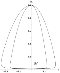
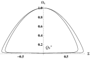
Figure 1: Projection of some orbits of the system (28)-(33) for the potential $V(\phi)=V_{0}\left[\cosh\left(\xi\phi\right)-1\right]$ with $\xi=1/2$ in the planes (a) $x-\Omega_{\lambda}$ and (b) $\Sigma-\Omega_{\lambda}$ for $\gamma=1$. This numerical elaboration shows that $Q_{9}^{+}$ is the local attractor.

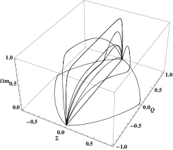
Figure 2: Projection of some orbits in the space $\Sigma,Q,\Omega_{m}.$ We choose the initial states near static solutions. This numerical elaboration shows the transition from the contracting de Sitter solution $Q_{9}^{-}$ (past attractor) to the expanding de Sitter solution $Q_{9}^{+}$ (future attractor).

Now, the inverted sinh-like potential

$$V(\phi)=V_{0}\sinh^{-\alpha}(\beta\phi),$$ (54)

has been widely investigated in the literature (e.g. Urena-Lopez and Matos (2000); Sahni and Starobinsky (2000); Pavluchenko (2003); Copeland et al. (2009)). The asymptotic properties of a cosmological model with a scalar field with such a potential have been investigated in the context of FRW brane in (Leyva et al., 2009).

The $f$-deviser corresponding to the potential (54) is given by

$$f(s)=\frac{s^{2}}{\alpha}-\alpha\beta^{2}.$$ (55)

The zeroes of this $f(s)$ function are

$$s^{*}=\pm\alpha\beta\quad f^{\prime}(s^{*})=\pm 2\beta.$$ (56)

The sufficient conditions for the existence of late-time attractors are fulfilled easily

• The scalar field-matter scaling solution $Q_{4}^{+}(\alpha\beta)$ is a late-time attractor provided $0<\gamma<\frac{4}{3},\beta<0,\alpha>-\frac{\sqrt{3\gamma}}{\beta},$ or $0<\gamma<\frac{4}{3},\alpha>\frac{\sqrt{3\gamma}}{\beta},\beta>0.$

• The scalar field-matter scaling solution $Q_{4}^{+}(-\alpha\beta)$ is a late-time attractor provided $0<\gamma<\frac{4}{3},\alpha<\frac{\sqrt{3\gamma}}{\beta},\beta>0$ or $0<\gamma<\frac{4}{3},\alpha>-\frac{\sqrt{3\gamma}}{\beta},\beta<0.$

• The solution dominated by scalar field $Q_{5}^{+}(\alpha\beta)$ is a late-time attractor provided $0<\gamma\leq\frac{4}{3},\beta<0,0<\alpha<-\frac{\sqrt{3\gamma}}{\beta}$ or $\frac{4}{3}<\gamma\leq 2,\beta<0,0<\alpha<-\frac{2}{\beta}$ or $0<\gamma\leq\frac{4}{3},0<\alpha<\frac{\sqrt{3\gamma}}{\beta},\beta>0$ or $\frac{4}{3}<\gamma\leq 2,0<\alpha<\frac{2}{\beta},\beta>0;$

• The solution dominated by scalar field $Q_{5}^{+}(-\alpha\beta)$ is a late-time attractor provided $0<\gamma\leq\frac{4}{3},\beta>0,0<\alpha<\frac{\sqrt{3\gamma}}{\beta}$ or $\frac{4}{3}<\gamma\leq 2,\beta>0,0<\alpha<\frac{2}{\beta}$ or $0<\gamma\leq\frac{4}{3},0<\alpha<-\frac{\sqrt{3\gamma}}{\beta},\beta<0$ or $\frac{4}{3}<\gamma\leq 2,0<\alpha<-\frac{2}{\beta},\beta<0;$

• The de Sitter solution $Q_{9}^{+}$ is the late time attractor provided $f(0)=-\alpha\beta^{2}>0.$

• $Q_{11}^{-}$ is stable for $\gamma>1.$

• The scalar field- dark radiation scaling solution
  $Q_{12}^{+}(\alpha\beta)$ is a late-time attractor for $\frac{4}{3}<\gamma\leq 2,\alpha\beta>2,\beta>0.$

• The scalar field- dark radiation scaling solution
  $Q_{12}^{+}(-\alpha\beta)$ is a late-time attractor for $\frac{4}{3}<\gamma\leq 2,\alpha\beta<-2,\beta<0.$

The past attractors of the system are as follows.

• The scalar field-matter scaling solution $Q_{4}^{-}(\alpha\beta)$ is the past attractor provided $0<\gamma<\frac{4}{3},\beta<0,\alpha>-\frac{\sqrt{3\gamma}}{\beta},$ or $0<\gamma<\frac{4}{3},\alpha>\frac{\sqrt{3\gamma}}{\beta},\beta>0.$

• The scalar field-matter scaling solution $Q_{4}^{-}(-\alpha\beta)$ is the past attractor provided $0<\gamma<\frac{4}{3},\alpha<\frac{\sqrt{3\gamma}}{\beta},\beta>0$ or $0<\gamma<\frac{4}{3},\alpha>-\frac{\sqrt{3\gamma}}{\beta},\beta<0.$

• The solution dominated by scalar field $Q_{5}^{-}(\alpha\beta)$ is the past attractor provided $0<\gamma\leq\frac{4}{3},\beta<0,0<\alpha<-\frac{\sqrt{3\gamma}}{\beta}$ or $\frac{4}{3}<\gamma\leq 2,\beta<0,0<\alpha<-\frac{2}{\beta}$ or $0<\gamma\leq\frac{4}{3},0<\alpha<\frac{\sqrt{3\gamma}}{\beta},\beta>0$ or $\frac{4}{3}<\gamma\leq 2,0<\alpha<\frac{2}{\beta},\beta>0;$

• The solution dominated by scalar field $Q_{5}^{-}(-\alpha\beta)$ is the past attractor provided $0<\gamma\leq\frac{4}{3},\beta>0,0<\alpha<\frac{\sqrt{3\gamma}}{\beta}$ or $\frac{4}{3}<\gamma\leq 2,\beta>0,0<\alpha<\frac{2}{\beta}$ or $0<\gamma\leq\frac{4}{3},0<\alpha<-\frac{\sqrt{3\gamma}}{\beta},\beta<0$ or $\frac{4}{3}<\gamma\leq 2,0<\alpha<-\frac{2}{\beta},\beta<0;$

• The de Sitter solution $Q_{9}^{-}$ is the past attractor provided $f(0)=-\alpha\beta^{2}>0.$

• $Q_{11}^{+}$ is unstable for $\gamma>1.$

• The scalar field- dark radiation scaling solution
  $Q_{12}^{-}(\alpha\beta)$ is a past attractor for $\frac{4}{3}<\gamma\leq 2,\alpha\beta>2,\beta>0.$

• The scalar field- dark radiation scaling solution
  $Q_{12}^{-}(-\alpha\beta)$ is the past attractor for $\frac{4}{3}<\gamma\leq 2,\alpha\beta<-2,\beta<0.$

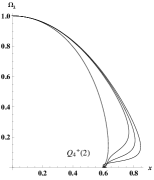
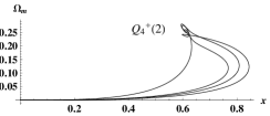
Figure 3: Projection of some orbits in the phase space of (28)-(33) for the potential $V(\phi)=V_{0}\sinh^{-\alpha}(\beta\phi)$ with $\alpha=1/2,\beta=4$ and $\gamma=1$ in the planes (a) $x-\Omega_{\lambda}$ and (b) $x-\Omega_{m}$. We set $Q=+1$ for the numerical simulation. This numerical elaboration shows that $Q_{4}^{+}(2)$ is the future attractor.

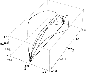
Figure 4: Projection of some orbits in the phase space of (28)-(33) for the potential $V(\phi)=V_{0}\sinh^{-\alpha}(\beta\phi)$ with $\alpha=1/2,\beta=4$ and $\gamma=1$ in the subspace $(\Sigma,Q,\Omega_{m})$. We choose the initial states near static solutions. This numerical elaboration illustrate the transition for the contracting scalar-field matter scaling solution $Q_{4}^{-}(2)$ (past attractor) to the expanding one $Q_{4}^{+}(2)$ (future attractor).

Figure 5: Transition from expansion ($Q>0$) to contraction ($Q<0$) and then back to expansion ($Q>0$), that is a cosmological turnaround and a bounce for the potential $V(\phi)=V_{0}\sinh^{-\alpha}(\beta\phi)$ with $\alpha=1/2,\beta=4$. The left panel corresponds to the projection of an orbit in the plane $x$-$Q$, while the right panel shows $\hat{Q}\equiv 10Q$ vs $\tau$, in order to illustrate that $Q$ change its sign twice during the evolution. We choose the initial condition $Q(0)=0.9,x(0)=0.6,\Omega_{m}(0)=0.25,\Omega_{\lambda}(0)=0,\Sigma(0)=0,s(0)=2.0.$

In the figures 3, 4 and 5 are presented some orbits in the phase space of (28)-(33) for the potential $V(\phi)=V_{0}\sinh^{-\alpha}(\beta\phi)$ with $\alpha=1/2,\beta=4$ and $\gamma=1$. In figure 3 we set $Q=+1$ for the numerical simulation. This numerical elaboration reveals that $Q_{4}^{+}(2)$ is the future attractor. In figure 4 we present a projection of some orbits in the subspace $(\Sigma,Q,\Omega_{m})$. We choose the initial states near the static solutions. This numerical elaboration illustrates the transition for the contracting scalar-field matter scaling solution $Q_{4}^{-}(2)$ (past attractor) to the expanding one $Q_{4}^{+}(2)$ (future attractor). As can be seen in the figures, the static solutions play an important role in the transition from contracting to expanding solutions and viceversa. In figure 5 we show the transition from expansion to contraction and then back to expansion, that is a cosmological turnaround and a cosmological bounce, for the solutions of (28)-(33), for the potential $V(\phi)=V_{0}\sinh^{-\alpha}(\beta\phi)$ with $\alpha=1/2,\beta=4$ and $\gamma=1$. The left panel corresponds to the projection of an orbit in the plane $x$-$Q$, while the right panel shows $\hat{Q}\equiv 10Q$ vs $\tau$ in order to illustrate that $Q$ change its sign twice during the evolution. We choose the initial condition $Q(0)=0.9,x(0)=0.6,\Omega_{m}(0)=0.25,\Omega_{\lambda}(0)=0,\Sigma(0)=0,s(0)=2.0.$

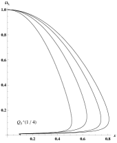
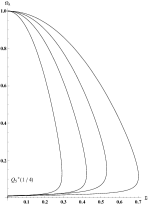
Figure 6: Some orbits of the phase space of (28)-(33) for the potential $V(\phi)=V_{0}\sinh^{-\alpha}(\beta\phi)$ with $\alpha=\beta=1/2$ and $\gamma=1$. Projection in the planes (a) $x-\Omega_{\lambda}$ and (b) $\Sigma-\Omega_{\lambda}$ (We set $Q=+1$ for the numerical simulation).

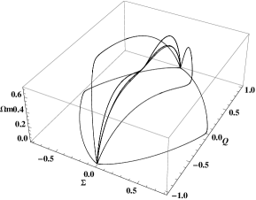
Figure 7: Some orbits in the projection $(\Sigma,Q,\Omega_{m})$ of the phase space of (28)-(33) for the potential $V(\phi)=V_{0}\sinh^{-\alpha}(\beta\phi)$ with $\alpha=\beta=1/2$ and $\gamma=1$. We choose initial states near the static solutions. This numerical elaboration shows the transition from the contracting scalar field dominated solution $Q_{5}^{-}(1/4)$ to the expanding one $Q_{5}^{+}(1/4)$.

In figures 6 and 7 are presented some orbits in the phase space of (28)-(33) for the potential $V(\phi)=V_{0}\sinh^{-\alpha}(\beta\phi)$ with $\alpha=\beta=1/2$ and $\gamma=1$. In figure 6 we set $Q=+1$ for the numerical simulation and we present the projection in the planes $x-\Omega_{\lambda}$ and $\Sigma-\Omega_{\lambda}.$ In this case the future attractor is the isotropic solution dominated by scalar field $Q_{5}^{+}(1/4)$, also this solution corresponds to an accelerated expansion rate since $s^{*}=1/4<\sqrt{2}$. In figure 7 are presented some orbits in the projection $(\Sigma,Q,\Omega_{m})$. This numerical elaboration shows the transition from the contracting scalar field dominated solution $Q_{5}^{-}(1/4)$ to the expanding one $Q_{5}^{+}(1/4)$. We choose the initial states near the static solutions.

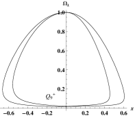
(a)

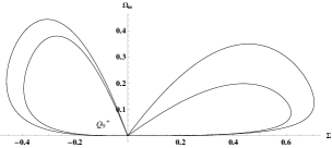
(b)

Figure 8: Some orbits of the phase space of (28)-(33) for the potential $V(\phi)=V_{0}\sinh^{-\alpha}(\beta\phi)$ with $\alpha=-1/2,\beta=-1/4$ and $\gamma=1$. Projection in the planes (a) $x-\Omega_{\lambda}$ and (b) $\Sigma-\Omega_{m}.$ We set $Q=+1$ for the numerical simulation.

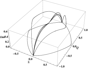
Figure 9: Some orbits in the subspace $(\Sigma,Q,\Omega_{m})$, $Q\neq+1$ of the phase space of (28)-(33) for the potential $V(\phi)=V_{0}\sinh^{-\alpha}(\beta\phi)$ with $\alpha=-1/2,\beta=-1/4$ and $\gamma=1$. We choose the initial states near static solutions. This numerical elaboration illustrate the transition for the contracting de Sitter solution $Q_{9}^{-}$ (past attractor) to the expanding de Sitter solution $Q_{9}^{+}$ (future attractor).

In figures 8 and 9 are showed some numerical integrations for the system (28)-(33) for the function (55) with $\alpha=-1/2,\beta=-1/4$. In this case the local attractor is the solution dominated by the potential energy of the scalar field $Q_{9}^{+}$ (de Sitter attractor). The past attractor is $Q_{9}^{-}.$ This numerical elaboration illustrate the transition from contracting to expanding solutions and viceversa that is not allowed for Bianchi I branes with positive Dark Radiation term (${\cal U}>0$).

VIII Conclusions

In this paper we have presented a full phase space analysis of a model consisting of a quintessence field with an arbitrary potential and a perfect fluid trapped in a Randall-Sundrum’s Braneworld of type 2. We have considered a homogeneous but anisotropic Bianchi I brane geometry. Moreover, we have also included the effect of the projection of the five-dimensional Weyl tensor onto the three-brane in the form of a negative dark radiation term.

We have discussed a general method for the treatment of the potential, called “Method of $f$-devisers”. Combining this method with some tools from the Theory of Dynamical Systems, we have obtained general conditions which have to be satisfied by the potential (encoded in the mathematical properties of the key $f(s)$-functions) in order to obtain the stability conditions of standard 4D and non-standard 5D de Sitter solutions.

We have presented general conditions under the potential for the stability of standard 4D de Sitter solutions. We proved that the de Sitter solutions with 5D corrections are stable against the perturbations introduced here, but are unstable against small perturbations of $V/(3H^{2}).$ This fact does not conflict with our previous results for BI branes with positive dark radiation term. Also, we presented the stability conditions for both scalar field-matter scaling solutions, for scalar field-dark radiation scaling solutions and scalar field-dominated solutions. The shear-dominated solutions are always unstable (contracting shear-dominated solutions are of saddle type). Also, we have shown that for all possible late time stable expanding solutions (attractors) the isotropization has been archived independently of the initial conditions, in all cases, with observational parameters in concordance with observations.

The main ansatz of our research is the assumption over the sign of Dark Radiation. If was shown that for ${\cal U}<0$, the ever-expanding models could potentially re-collapse. Additionally, our system admits a large class of static solutions that are of saddle type allowing the transition from contracting to expanding models and viceversa. Thus, a new feature of this scenario is the existence of a bounce and a turnaround, which leads to cyclic behavior. This features are not allowed in Bianchi I branes with positive dark radiation term. This is an important cosmological result in our scenario, that is a consequence of the negativeness of the dark radiation. In this direction, it is worth exploring in detail the current magnitudes and sign of the Dark Radiation, for a Bianchi I braneworld, allowed by cosmological observations since it is an study that is absent, to our knowledge, in the literature. For this latter purpose, not only the well-establish tests of SNe, BAO, H(z), CMB and BBN would provide significant constraints, but also the recent results from multi-wavelength observation could improved the observational study. More precisely, the recent detection of the cosmic $\gamma$-ray horizon from multi-wavelength observation of blazars (Dominguez et al., 2013), using the data from the Fermi satellite and the Imaging Atmospheric Cherenkov Telescopes, allowed a new measurement of the Hubble constant (Dominguez and Prada, 2013) and opening a new door to, not only, control systematic uncertainties associated with determinations of the Hubble constant (Suyu et al., 2012; Dominguez and Prada, 2013), but also to impose new constraints over dark energy and neutrino physics (Weinberg et al., 2013; Suyu et al., 2012; Freedman and Madore, 2010). Is expected that in the near future, with more data from the upcoming generation of multi-wavelength observation/ instrumentation facilities planned worldwide such as the Cherenkov Telescope Array, this kind of estimation will become more competitive at the level of other techniques such as CMB, BAO etc.

Finally, in order to be more transparent, we have illustrated our main results for the specific potentials $V\propto\sinh^{-\alpha}(\beta\phi)$ and $V\propto\left[\cosh\left(\xi\phi\right)-1\right]$ which have simple $f$-devisers.

Appendix A Stability of static solutions

As we commented before, the system (29)-(33) admits eighteen classes of (curves of) fixed points corresponding to static solutions, i.e., having $Q=0,$ that is with $H=0.$ Their coordinates in the phase space and their existence conditions are displayed in table (2). In the table 5 are presented the corresponding eigenvalues, where $\lambda_{1}(\epsilon,\Sigma_{c}),\lambda_{2}(\epsilon,\Sigma_{c}),\lambda_{3}(\epsilon,\Sigma_{c}),$ $\lambda_{4}(\epsilon,\Sigma_{c})$ are the roots of the equation

$$\lambda^{4}+\lambda^{3}\sqrt{4-6\Sigma_{c}^{2}}\epsilon f^{\prime}(0)+\lambda^{2}\left[f(0)-4\right]-4\lambda\sqrt{4-6\Sigma_{c}^{2}}\epsilon f^{\prime}(0)-6f(0)\Sigma_{c}^{2}=0,$$

and $\mu_{1}(\epsilon,\Sigma_{c}),\mu_{2}(\epsilon,\Sigma_{c}),\mu_{3}(\epsilon,\Sigma_{c}),$ $\mu_{4}(\epsilon,\Sigma_{c})$ are the roots of the equation

$$\mu^{4}+\sqrt{2}\mu^{3}\Sigma_{c}\epsilon f^{\prime}(0)+\mu^{2}\left[2(f(0)+4){\Sigma_{c}}^{2}-8\right]+8\sqrt{2}\mu\Sigma_{c}\left(\Sigma_{c}^{2}-1\right)\epsilon f^{\prime}(0)+4f(0)\Sigma_{c}^{2}\left(\Sigma_{c}^{2}-2\right)=0.$$

Table 5: Eigenvalues for the critical points in table (2). Are used the notations $g_{1}(\gamma,\Omega_{\lambda},\Sigma)=\frac{\sqrt{-3\gamma\left(3\Sigma^{2}-2\right)\left(-\Sigma^{2}+\Omega_{\lambda}+1\right)^{2}+18\Sigma^{6}-44\Sigma^{4}+2\Sigma^{2}(\Omega_{\lambda}(9\Omega_{\lambda}+2)+17)-8\left(\Omega_{\lambda}^{2}+1\right)}}{-\Sigma^{2}+\Omega_{\lambda}+1},$ $g_{2}(\gamma,\Omega_{\lambda},\Sigma)=\frac{\sqrt{f(0)}\sqrt{\Sigma^{2}+\Omega_{\lambda}-1}\sqrt{3\gamma\left(-\Sigma^{2}+\Omega_{\lambda}+1\right)+6\Sigma^{2}-4}}{\sqrt{\gamma}\sqrt{-\Sigma^{2}+\Omega_{\lambda}+1}},$ $g_{3}(\gamma,x,\Omega_{\lambda},\Sigma)=-\frac{9}{2}\left(\gamma^{2}(\Omega_{\lambda}-1)\Omega_{\lambda}+(\gamma-2)^{2}\Sigma^{4}-(\gamma-2)\Sigma^{2}(2\gamma\Omega_{\lambda}+\gamma-2)\right)-\frac{9(\gamma-2)^{2}x^{4}\left(\Sigma^{4}-2\Sigma^{2}(\Omega_{\lambda}+1)+\Omega_{\lambda}^{2}+1\right)}{2\left(\Sigma^{2}+\Omega_{\lambda}-1\right)^{2}}-\frac{9(\gamma-2)x^{2}\left(-\Omega_{\lambda}\left(4(\gamma-1)\Sigma^{2}+\gamma+2\right)+(\gamma-2)\left(2\Sigma^{4}-3\Sigma^{2}+1\right)+2\gamma\Omega_{\lambda}^{2}\right)}{2\left(\Sigma^{2}+\Omega_{\lambda}-1\right)},$
$g_{4}(\gamma,x,\Omega_{\lambda})=\frac{3\sqrt{-\gamma^{2}(\Omega_{\lambda}-1)^{3}\Omega_{\lambda}-(\gamma-2)^{2}x^{4}\left(\Omega_{\lambda}^{2}+1\right)-(\gamma-2)x^{2}(\Omega_{\lambda}-1)\left(2\gamma\Omega_{\lambda}^{2}-(\gamma+2)\Omega_{\lambda}+\gamma-2\right)}}{\sqrt{2}(\Omega_{\lambda}-1)}.$

Labels	Eigenvalues
$E_{1}^{\pm}$	$\left\{-2,2,0,0,-\sqrt{f(0)}\sqrt{3\Omega_{\lambda c}-1},\sqrt{f(0)}\sqrt{3\Omega_{\lambda c}-1}\right\}$
$E_{2}$	$\left\{0,0,0,0,-\frac{3}{2}\sqrt{1-\cos(4u)},\frac{3}{2}\sqrt{1-\cos(4u)}\right\}$
$E_{3}$	$\left\{0,0,-g_{1}(\gamma,\Omega_{\lambda c},\Sigma_{c}),g_{1}(\gamma,\Omega_{\lambda c},\Sigma_{c}),-g_{2}(\gamma,\Omega_{\lambda c},\Sigma_{c}),g_{2}(\gamma,\Omega_{\lambda c},\Sigma_{c})\right\}$
$E_{4}$	$\left\{0,0,0,0,-\sqrt{-9\gamma^{2}+9(\gamma-2)(\gamma-1)\Sigma_{c}^{2}+18\gamma-8},\sqrt{-9\gamma^{2}+9(\gamma-2)(\gamma-1)\Sigma_{c}^{2}+18\gamma-8}\right\}$
$E_{5}$	$\left\{0,0,-\sqrt{g_{3}(\gamma,x_{c},\Omega_{\lambda c},\Sigma_{c})},\sqrt{g_{3}(\gamma,x_{c},\Omega_{\lambda c},\Sigma_{c})},-\sqrt{6}s^{*}x_{c},-\sqrt{6}x_{c}f^{\prime}\left(s^{*}\right)\right\}$
$E_{6}^{\epsilon}$	$\left\{0,0,\lambda_{1}(\epsilon,\Sigma_{c}),\lambda_{2}(\epsilon,\Sigma_{c}),\lambda_{3}(\epsilon,\Sigma_{c}),\lambda_{4}(\epsilon,\Sigma_{c})\right\}$
$E_{7}^{\epsilon}$	$\left\{0,0,\mu_{1}(\epsilon,\Sigma_{c}),\mu_{2}(\epsilon,\Sigma_{c}),\mu_{3}(\epsilon,\Sigma_{c}),\mu_{4}(\epsilon,\Sigma_{c})\right\}$
$E_{8}$	$\left\{0,0,-g_{4}(\gamma,x_{c},\Omega_{\lambda c}),g_{4}(\gamma,x_{c},\Omega_{\lambda c}),-\sqrt{6}s^{*}x_{c},-\sqrt{6}x_{c}f^{\prime}\left(s^{*}\right)\right\}$
$E_{9}$	$\left\{0,0,-\frac{\sqrt{6\gamma(\Omega_{\lambda}+1)^{2}-8\left(\Omega_{\lambda}^{2}+1\right)}}{\Omega_{\lambda}+1},\frac{\sqrt{6\gamma(\Omega_{\lambda}+1)^{2}-8\left(\Omega_{\lambda}^{2}+1\right)}}{\Omega_{\lambda}+1},-\frac{\sqrt{f(0)}\sqrt{\Omega_{\lambda}-1}\sqrt{3\gamma(\Omega_{\lambda}+1)-4}}{\sqrt{\gamma}\sqrt{\Omega_{\lambda}+1}},\frac{\sqrt{f(0)}\sqrt{\Omega_{\lambda}-1}\sqrt{3\gamma(\Omega_{\lambda}+1)-4}}{\sqrt{\gamma}\sqrt{\Omega_{\lambda}+1}}\right\}$
$E_{10}^{\epsilon}$	$\left\{0,0,-\epsilon\sqrt{2}\sqrt{\frac{3\gamma-2}{\gamma-2}}s^{*}\Sigma_{c},\sqrt{2}\sqrt{\gamma\left(9\Sigma^{2}-6\right)-4\Sigma^{2}+4},-\sqrt{2}\sqrt{\gamma\left(9\Sigma^{2}-6\right)-4\Sigma^{2}+4},-\epsilon\sqrt{2}\sqrt{\frac{3\gamma-2}{\gamma-2}}\Sigma_{c}f^{\prime}\left(s^{*}\right)\right\}$
$E_{11}$	$\left\{0,0,-\sqrt{\gamma\left(6-9\Sigma_{c}^{2}\right)+10\Sigma_{c}^{2}-4},\sqrt{\gamma\left(6-9\Sigma_{c}^{2}\right)+10\Sigma_{c}^{2}-4},-\frac{\sqrt{2-3\gamma}\sqrt{f(0)}\Sigma_{c}}{\sqrt{\gamma}},\frac{\sqrt{2-3\gamma}\sqrt{f(0)}\Sigma_{c}}{\sqrt{\gamma}}\right\}$
$E_{12}$	$\left\{0,0,-\sqrt{\gamma\left(6-9\Sigma^{2}\right)+18\Sigma^{2}-8},\sqrt{\gamma\left(6-9\Sigma^{2}\right)+18\Sigma^{2}-8},-\frac{\sqrt{f(0)}\sqrt{3(\gamma-2)\Sigma^{2}-3\gamma+4}}{\sqrt{\gamma}},\frac{\sqrt{f(0)}\sqrt{3(\gamma-2)\Sigma^{2}-3\gamma+4}}{\sqrt{\gamma}}\right\}$
$E_{13}^{\epsilon}$	$\left\{0,0,\sqrt{4-3\gamma},-\sqrt{4-3\gamma},-\frac{\sqrt{2}\sqrt{4-3\gamma}s^{*}\epsilon}{\sqrt{2-\gamma}},-\sqrt{2}\sqrt{\frac{3\gamma-4}{\gamma-2}}\epsilon f^{\prime}\left(s^{*}\right)\right\}$

Now let us comment on the stability of the first order perturbations of (28)-(33) near the critical points showed in table 2.

The line of fixed points $E_{1}$ is non-hyperbolic. However, the points located at the curve behaves as saddle points since its matrix of perturbations admits at least two real eigenvalues of different signs.

The one-parametric line of fixed points $E_{2}$ has two real eigenvalues of different signs provided $\cos(4u)\neq 1.$ In this case, although non-hyperbolic, it behaves as a set of saddle points. For $u\in\left\{\frac{\pi}{2},\frac{3\pi}{2}\right\}$ all the eigenvalues are zero. In this case we need to resort to a numerical elaboration.

$g_{1}(\gamma,\Omega_{\lambda},\Sigma)$ is always real-valued for the allowed values of the phase space variables and the allowed range for the free parameters. Then, although non-hyperbolic, the 2D set of fixed points $E_{3}$ is of saddle type.

The eigenvalues associated to the one-parametric curve of fixed points $E_{4}$ are always reals for the allowed values of the phase space variables and the allowed range for the free parameters. Thus, although non-hyperbolic, it behaves as a saddle point. For the allowed values of the phase space variables and the allowed range for the free parameters the expression $g_{3}(\gamma,x_{c},\Omega_{\lambda c},\Sigma_{c})\geq 0.$ If it is strictly positive, then the fixed points located in the 2D invariant set $E_{5}$ behaves as saddle points.

The eigenvalues of the perturbation matrix associated to $E_{6}^{\epsilon}$ are $\left\{0,0,\lambda_{1}(\epsilon,\Sigma_{c}),\lambda_{2}(\epsilon,\Sigma_{c}),\lambda_{3}(\epsilon,\Sigma_{c}),\lambda_{4}(\epsilon,\Sigma_{c})\right\}$ where $\lambda_{1}(\epsilon,\Sigma_{c}),\lambda_{2}(\epsilon,\Sigma_{c}),\lambda_{3}(\epsilon,\Sigma_{c})$ and $\lambda_{4}(\epsilon,\Sigma_{c})$ are the roots of the polynomial equation with real coefficients:

$$\lambda^{4}+\lambda^{3}\sqrt{4-6\Sigma_{c}^{2}}\epsilon f^{\prime}(0)+\lambda^{2}\left[f(0)-4\right]-4\lambda\sqrt{4-6\Sigma_{c}^{2}}\epsilon f^{\prime}(0)-6f(0)\Sigma_{c}^{2}=0.$$ (57)

• For $f^{\prime}(0)\neq 0,f(0)<0,$ equation (57) has only two changes of signs in the sequence of its coefficients. Hence, using the Descartes’s rule, we conclude that for this range of the parameters, there is zero or two positive roots of (57). Substituting $\lambda$ by $-\lambda$ in (57) and applying the same rule we have zero or two negative roots of (57) for $f^{\prime}(0)\neq 0,f(0)<0.$ If all of them are complex conjugated, we need to resort to numerical investigation. If none of them are complex conjugated, then the curve of fixed points $E_{6}^{\epsilon}$ consists of saddle points.

• For $\epsilon f^{\prime}(0)>0,f(0)>0,$ equation (57) has only one change of sign in the sequence of its coefficients. Hence, using the Descartes’s rule, we conclude that for this range of the parameters, there is one positive root of (57). Substituting $\lambda$ by $-\lambda$ in (57) and applying the same rule we have three negative roots of (57) for $\epsilon f^{\prime}(0)>0,f(0)>0.$ In summary, for $\epsilon f^{\prime}(0)>0,f(0)>0,$ at least two eigenvalues of the linear perturbation matrix of $E_{6}^{+}$ are real of different signs. In this case the curve of fixed points $E_{6}^{\epsilon}$ consists of saddle points.

• For $\epsilon f^{\prime}(0)<0,f(0)>0,$ equation (57) has three changes of sign in the sequence of its coefficients. Hence, using the Descartes’s rule, we conclude that for this range of the parameters, there are three positive roots of (57). Substituting $\lambda$ by $-\lambda$ in (57) and applying the same rule we have only one negative root of (57) for $\epsilon f^{\prime}(0)<0,f(0)>0.$ In this case the curve of fixed points $E_{6}^{\epsilon}$ consists of saddle points.

• For $f^{\prime}(0)=f(0)=0$ the non null eigenvalues are $-2,2;$ for $f^{\prime}(0)=0,f(0)\neq 0,$ the non null eigenvalues are:
  $\displaystyle\pm\frac{\sqrt{-\sqrt{24f(0)\Sigma_{c}^{2}+(f(0)-4)^{2}}-f(0)+4}}{\sqrt{2}},\;\;\;\;\pm\frac{\sqrt{\sqrt{24f(0)\Sigma_{c}^{2}+(f(0)-4)^{2}}-f(0)+4}}{\sqrt{2}};$
  and for $f^{\prime}(0)\neq 0,f(0)=0,$ the non null eigenvalues are $-2,2,-\epsilon\sqrt{4-6\Sigma_{c}^{2}}f^{\prime}(0).$ Thus, in both cases $E_{6}^{\pm}$ consists of saddle points.

The eigenvalues of the perturbation matrix associated to $E_{7}^{\epsilon}$ are $\left\{0,0,\mu_{1}(\epsilon,\Sigma_{c}),\mu_{2}(\epsilon,\Sigma_{c}),\mu_{3}(\epsilon,\Sigma_{c}),\mu_{4}(\epsilon,\Sigma_{c})\right\}$ where $\mu_{1}(\epsilon,\Sigma_{c}),\mu_{2}(\epsilon,\Sigma_{c}),\mu_{3}(\epsilon,\Sigma_{c})$ and $\mu_{4}(\epsilon,\Sigma_{c})$ are the roots of the polynomial equation with real coefficients:

$$\mu^{4}+\sqrt{2}\mu^{3}\Sigma_{c}\epsilon f^{\prime}(0)+\mu^{2}\left[2(f(0)+4){\Sigma_{c}}^{2}-8\right]+8\sqrt{2}\mu\Sigma_{c}\left(\Sigma_{c}^{2}-1\right)\epsilon f^{\prime}(0)+4f(0)\Sigma_{c}^{2}\left(\Sigma_{c}^{2}-2\right)=0.$$ (58)

• For $\epsilon f^{\prime}(0)<0,f(0)<0,-\frac{1}{\sqrt{2}}<\Sigma_{c}<0$ or $\epsilon f^{\prime}(0)>0,f(0)<0,0<\Sigma_{c}<\frac{1}{\sqrt{2}},$ or $\epsilon f^{\prime}(0)<0,f(0)<0,0<\Sigma_{c}<\frac{1}{\sqrt{2}},$ or $\epsilon f^{\prime}(0)>0,f(0)<0,-\frac{1}{\sqrt{2}}<\Sigma_{c}<0,$ the equation (58) has only two changes of signs in the sequence of its coefficients. Hence, using the Descartes’s rule, we conclude that for this range of the parameters, there is zero or two positive roots of (58). Substituting $\mu$ by $-\mu$ in (58) and applying the same rule we have zero or two negative roots of (58) for the same values of the free parameters. If all of them are complex conjugated, we need to resort to numerical investigation. If none of them are complex conjugated, then the curve of fixed points $E_{7}^{\epsilon}$ consists of saddle points.

• For $f(0)>0,\epsilon f^{\prime}(0)>0,0<\Sigma_{c}<\frac{1}{\sqrt{2}}$ or $f(0)>0,\epsilon f^{\prime}(0)<0,\frac{1}{\sqrt{2}}<\Sigma_{c}<0,$ equation (58) has only one change of sign in the sequence of its coefficients. Hence, using the Descartes’s rule, we conclude that for this range of the parameters, there is one positive root of (58). Substituting $\mu$ by $-\mu$ in (58) and applying the same rule we have three negative roots of (58) for the same values of the parameters. In this case the curve of fixed points $E_{7}^{\epsilon}$ consists of saddle points.

• For $f(0)>0,0<\Sigma_{c}<\frac{1}{\sqrt{2}},\epsilon f^{\prime}(0)<0$ or $f(0)>0,-\frac{1}{\sqrt{2}}<\Sigma_{c}<0,\epsilon f^{\prime}(0)>0$ equation (58) has three changes of sign in the sequence of its coefficients. Hence, using the Descartes’s rule, we conclude that for this range of the parameters, there are three positive roots of (58). Substituting $\mu$ by $-\mu$ in (58) and applying the same rule we have only one negative root of (58) for the same values of the parameters. In this case the curve of fixed points $E_{7}^{\epsilon}$ consists of saddle points.

• For $f^{\prime}(0)=f(0)=0$ the non null eigenvalues are $2\sqrt{2}\sqrt{1-\Sigma_{c}^{2}},-2\sqrt{2}\sqrt{1-\Sigma_{c}^{2}};$ for $f^{\prime}(0)=0,f(0)\neq 0,$ the non null eigenvalues are $\pm\sqrt{4-(f(0)+4)\Sigma_{c}^{2}-\sqrt{\Delta}}$, and $\pm\sqrt{4-(f(0)+4)\Sigma_{c}^{2}+\sqrt{\Delta}},$ where $\Delta=(f(0)(f(0)+4)+16)\Sigma_{c}^{4}-32\Sigma_{c}^{2}+16$; and for $f^{\prime}(0)\neq 0,f(0)=0,$ the non null eigenvalues are $-\sqrt{2}\Sigma_{c}\epsilon f^{\prime}(0),\pm 2\sqrt{2-2\Sigma_{c}^{2}}.$ Thus, in both cases $E_{7}^{\pm}$ consists of saddle points.

Observe that $g_{4}(\gamma,x,\Omega_{\lambda})$ is always real-valued for the allowed values of the phase space variables and the allowed range for the free parameters. Then, although non-hyperbolic, $E_{8}$ behaves as a set of saddle points.

When $\displaystyle\Omega_{\lambda c}\neq 1,\;\;\;\frac{\sqrt{6\gamma(\Omega_{\lambda}+1)^{2}-8\left(\Omega_{\lambda}^{2}+1\right)}}{\Omega_{\lambda}+1}$ is real valued, in this case the fixed points in the line $E_{9}$ behaves as saddle points.

For $\Sigma_{c}\neq 0,$ $\sqrt{2}\sqrt{\gamma\left(9\Sigma^{2}-6\right)-4\Sigma^{2}+4}$ is real-valued, in this case the fixed points in the line $E_{10}$ behaves as saddle points.

For $\Sigma_{c}\neq 0,$ the linear perturbation matrix evaluated at $E_{11}$ has at least two real eigenvalues of different signs, thus, the fixed points in the line $E_{11}$ behaves as saddle points.

Observe that the line $E_{9}$ and the line $E_{11}$ contains the special point with coordinates $F:(Q=0,x=0,\Omega_{m}=0,\Omega_{\lambda}=1,\Sigma=0)$ in the first case when $\Omega_{\lambda c}\rightarrow 1$ whereas in the second case for $\Sigma_{c}\rightarrow 0.$ Taking in both cases the proper limits we have that the eigenvalues of the linearization for $F$ are $\left\{0,0,-\sqrt{6\gamma-4},\sqrt{6\gamma-4},0,0\right\}.$ Hence, for $\gamma>\frac{2}{3},$ $F$ is of saddle type, whereas for $\gamma<\frac{2}{3},$ there are two purely imaginary eigenvalues and the rest of the eigenvalues are zero. In this case we cannot say anything about its stability from the linearization and we need to resort to numerical inspection.

Observe that $\sqrt{\gamma\left(6-9\Sigma^{2}\right)+18\Sigma^{2}-8}$ is real-valued for the allowed values of the phase space variables and the allowed range for the free parameters. Thus, all the points located at the line $E_{12}$ behaves as saddle points.

For $0<\gamma<\frac{4}{3},$ $E_{13}^{\pm}$ behaves as a saddle point.

Appendix B Stability of expanding (contracting) solutions

Now let us comment on the stability of the first order perturbations of (28)-(33) near the critical points showed in table (3).

The line of singular points $Q_{1}^{\pm}$, although it is non-hyperbolic (actually, normally hyperbolic), behaves like a saddle point in the phase space of the RS model, since they have both nonempty stable and unstable manifolds (see the table 6). The class $Q_{1}^{+}$ is the analogous to the line denoted by $P_{1}$ in (Escobar et al., 2012b).

The singular points $Q_{2}^{\pm}(s^{*})$ and $Q_{3}^{\pm}(s^{*})$ are non-hyperbolic (these points are related to $P_{3}^{\pm}$ investigated in (Escobar et al., 2012b)), however they behave as saddle points since they have both nonempty stable and unstable manifolds (see the table 6).

The singular point $Q_{4}^{+}(s^{*})$ is the analogous to $P_{4}$ in (Escobar et al., 2012b). It is a stable node in the cases $0<\gamma\leq\frac{2}{9},s^{*}<-\sqrt{3\gamma},f^{\prime}\left(s^{*}\right)<0$ or $\frac{2}{9}<\gamma<\frac{4}{3},-\frac{2\sqrt{6}\gamma}{\sqrt{9\gamma-2}}\leq s^{*}<-\sqrt{3\gamma},f^{\prime}\left(s^{*}\right)<0,$ or $0<\gamma\leq\frac{2}{9},s^{*}>\sqrt{3\gamma},f^{\prime}\left(s^{*}\right)>0,$ or $\frac{2}{9}<\gamma<\frac{4}{3},\sqrt{3\gamma}<s^{*}\leq\frac{2\sqrt{6}\gamma}{\sqrt{9\gamma-2}},f^{\prime}\left(s^{*}\right)>0.$ It is a spiral stable point for
$\frac{2}{9}<\gamma<\frac{4}{3},s^{*}<-\frac{2\sqrt{6}\gamma}{\sqrt{9\gamma-2}},f^{\prime}\left(s^{*}\right)<0$ or $\frac{2}{9}<\gamma<\frac{4}{3},s^{*}>\frac{2\sqrt{6}\gamma}{\sqrt{9\gamma-2}},f^{\prime}\left(s^{*}\right)>0.$ In summary, it is stable for $0<\gamma<\frac{4}{3},s^{*}<-\sqrt{3\gamma},f^{\prime}\left(s^{*}\right)<0$ or $0<\gamma<\frac{4}{3},s^{*}>\sqrt{3\gamma},f^{\prime}\left(s^{*}\right)>0.$ Otherwise, it is a saddle point.

The singular point $Q_{4}^{-}(s^{*})$ is a local source under the same conditions for which $Q_{4}^{+}(s^{*})$ is stable.

The singular point $Q_{5}^{+}(s^{*})$ is the analogous to $P_{5}$ in (Escobar et al., 2012b). It is not hyperbolic for $s^{*}\in\left\{0,\pm\sqrt{6},\pm\sqrt{3\gamma},2\right\}$ or $f^{\prime}(s^{*})=0$. In the hyperbolic case, $Q_{5}^{+}(s^{*})$ is a stable node for $0<\gamma\leq\frac{4}{3},-\sqrt{3\gamma}<s^{*}<0,f^{\prime}\left(s^{*}\right)<0$ or $\frac{4}{3}<\gamma\leq 2,-2<s^{*}<0,f^{\prime}\left(s^{*}\right)<0$ or $0<\gamma\leq\frac{4}{3},0<s^{*}<\sqrt{3\gamma},f^{\prime}\left(s^{*}\right)>0$ or $\frac{4}{3}<\gamma\leq 2,0<s^{*}<2,f^{\prime}\left(s^{*}\right)>0;$ otherwise, it is a saddle point.

The singular point $Q_{5}^{-}(s^{*})$ is a local source under the same conditions for which $Q_{5}^{+}(s^{*})$ is stable.

For evaluating the Jacobian matrix, and obtaining their eigenvalues at the singular points $Q_{6}^{\pm},$ $Q_{7}^{\pm}$ and $Q_{11}^{\pm}$ we need to take the appropriate limits. The details on the stability analysis for $Q_{6}^{+}$ and $Q_{11}^{+}$ are offered in the Appendix C. The analysis of $Q_{7}^{+}$ is essentially the same as for $Q_{6}^{+}.$

The circles of critical points $Q_{8}^{\pm}$ are non-hyperbolic. Both solutions represents transient states in the evolution of the universe.

The singular point $Q_{9}^{\pm}$ and the line of critical points $Q_{10}^{\pm}$ are non-hyperbolic ($Q_{9}^{+}$ is the analogous of $P_{10}$ for $\Omega_{\lambda}=0$ while $Q_{10}^{+}$ is the analogous of $P_{10}$ for $\Omega_{\lambda}\neq 0$ in (Escobar et al., 2012b)). In the Appendix B.1 we analyze the stability of $Q_{9}^{+}$ by introducing a local set of coordinates adapted to the singular points. The non-hyperbolic fixed point $Q_{9}^{-},$ behaves as a past attractor.

The singular point $Q_{11}^{+}$ is the analogous of $P_{11}$ in (Escobar et al., 2012b), this point represents a 1D set of singular points such that ($\Omega_{\lambda}=1$), parametrized by the values of $s_{c}.$ It is normally hyperbolic.

The singular points $Q_{12}^{\pm}(s^{*})$ are non-hyperbolic for $s^{*}=0,\pm 2$, $\gamma=4/3$ or $f^{\prime}(s^{*})=0$. $Q_{12}^{+}(s^{*})$ is a stable node for $\frac{4}{3}<\gamma\leq 2,2<s^{*}\leq\frac{8}{\sqrt{15}},f^{\prime}\left(s^{*}\right)>0,$ a stable spiral for $\frac{4}{3}<\gamma\leq 2,s^{*}>\frac{8}{\sqrt{15}},f^{\prime}\left(s^{*}\right)>0.$ In summary, $Q_{12}^{+}(s^{*})$ is stable for $\frac{4}{3}<\gamma\leq 2,s^{*}>2,f^{\prime}\left(s^{*}\right)>0.$ Otherwise it is a saddle point. $Q_{12}^{-}(s^{*})$ is unstable for the same conditions for which $Q_{12}^{+}(s^{*})$ is stable.

The eigenvalues of the linear perturbation matrix evaluated at each of these critical points are displayed in the table 6.

Table 6: Eigenvalues for the critical points in table (3). We use the notations $K^{\pm}(\gamma,s^{*})=-\frac{3}{4}\left(2-\gamma\pm\frac{\sqrt{2-\gamma}\sqrt{{s^{*}}^{2}(2-9\gamma)+24\gamma^{2}}}{s^{*}}\right),$ $L^{\pm}(\Omega_{\lambda})=-\frac{1}{2}\left(3\pm\sqrt{12f(0)(\Omega_{\lambda}-1)+9}\right)$ and $M^{\pm}(s^{*})=\frac{1}{4}\left(-s^{*}\pm\sqrt{64-15\left(s^{*}\right)^{2}}\right),$ where $s^{*}$ denotes an $s$-value such that $f(s^{*})=0.$

Label	Eigenvalues
$Q_{1}^{\pm}$	$\left\{(3\gamma-4)\epsilon,\frac{3}{2}(\gamma-2)\epsilon,\frac{3}{2}(\gamma-2)\epsilon,-3\gamma\epsilon,3\gamma\epsilon,0\right\}$
$Q_{2}^{\pm}(s^{*})$	$\left\{2\epsilon,0,-6\epsilon,-3(\gamma-2)\epsilon,6\epsilon-\sqrt{6}s^{*},-\sqrt{6}f^{\prime}\left(s^{*}\right)\right\}$
$Q_{3}^{\pm}(s^{*})$	$\left\{2\epsilon,0,-6\epsilon,-3(\gamma-2)\epsilon,6\epsilon\sqrt{6}s^{*},\sqrt{6}f^{\prime}\left(s^{*}\right)\right\}$
$Q_{4}^{\pm}(s^{*})$	$\left\{-3\gamma\epsilon,\frac{3}{2}(\gamma-2)\epsilon,(3\gamma-4)\epsilon,\epsilon K^{+}(\gamma,s^{*}),\epsilon K^{-}(\gamma,s^{*}),-\frac{3\gamma\epsilon f^{\prime}\left(s^{*}\right)}{s^{*}}\right\}$
$Q_{5}^{\pm}(s^{*})$	$\left\{-\epsilon\left(s^{*}\right)^{2},\frac{1}{2}\left({s^{*}}^{2}-6\right)\epsilon,\frac{1}{2}\left({s^{*}}^{2}-6\right)\epsilon,\left({s^{*}}^{2}-3\gamma\right)\epsilon,({s^{*}}^{2}-4)\epsilon,-\epsilon s^{*}f^{\prime}\left(s^{*}\right)\right\}$
$Q_{6}^{\pm}$	$\{6\epsilon,6\epsilon,2\epsilon,0,0,3(2-\gamma)\epsilon\}$
$Q_{7}^{\pm}$	$\{6\epsilon,6\epsilon,2\epsilon,0,0,3(2-\gamma)\epsilon\}$
$Q_{8}^{\pm}(s^{*})$	$\left\{0,6\epsilon-\sqrt{6}s\cos(u),-3(\gamma-2)\epsilon,2\epsilon,-6\epsilon,-\sqrt{6}\cos(u)f^{\prime}(s)\right\}$
$Q_{9}^{\pm}$	$\left\{-4\epsilon,-3\epsilon,0,0,\frac{1}{2}\left(-\sqrt{9-12f(0)}-3\right)\epsilon,\frac{1}{2}\left(\sqrt{9-12f(0)}-3\right)\epsilon\right\}$
$Q_{10}^{\pm}$	$\left\{-4\epsilon,-3\epsilon,0,-3\gamma\epsilon\Omega_{\lambda},\epsilon L^{+}(\Omega_{\lambda}),\epsilon L^{-}(\Omega_{\lambda})\right\}$
$Q_{11}^{\pm}$	$\left\{2(3\gamma-2)\epsilon,3(\gamma-1)\epsilon,3\gamma\epsilon,3\gamma\epsilon,3(\gamma-1)\epsilon,0\right\}$
$Q_{12}^{\pm}(s^{*})$	$\left\{-2s^{*}\epsilon,-\frac{s^{*}\epsilon}{2},\frac{1}{2}(4-3\gamma)s^{*}\epsilon,\epsilon M^{+}(s^{*}),\epsilon M^{-}(s^{*}),-2\epsilon f^{\prime}\left(s^{*}\right)\right\}$

B.1 De Sitter solutions.

To investigate the de Sitter solution $Q_{9}^{+},$ we introduce the local coordinates:

$$\left\{x,\Omega_{\lambda},Q-1,\Omega_{m},\Sigma,s\right\}=\epsilon\left\{\hat{x},\hat{\Omega}_{\lambda},\hat{Q},\hat{\Omega}_{m},\hat{\Omega}_{\sigma},\hat{s}\right\}+{\cal O}(\epsilon)^{2},$$ (59)

where $\epsilon$ is a small constant $\epsilon\ll 1.$ Then, we obtain the approximated system

$$\hat{Q}^{\prime}=-4\hat{Q},\;\hat{x}^{\prime}=\sqrt{\frac{3}{2}}\hat{s}-3\hat{x},\;\hat{\Omega}_{\lambda}^{\prime}=0,\;\hat{\Omega}_{m}^{\prime}=-3\gamma\hat{\Omega}_{m},\;\hat{\Omega}_{\sigma}^{\prime}=-3\hat{\Omega}_{\sigma},\;\hat{s}^{\prime}=-\sqrt{6}f(0)\hat{x}.$$ (60)

The system (60) admits the exact solution passing by ($\hat{Q}_{0},\hat{x}_{0},\hat{\Omega}_{\lambda 0},\hat{\Omega}_{m0},\hat{\Omega}_{\sigma 0},\hat{s}_{0}$) at $\tau=0$ given by

$$\hat{Q}(\tau)=\hat{Q}_{0}e^{-4\tau},\;\hat{x}(\tau)=\frac{1}{2}\hat{x}_{0}e^{-\frac{1}{2}\tau(\vartheta+3)}\left(e^{\tau\vartheta}+1\right)-\frac{e^{-\frac{1}{2}\tau(\vartheta+3)}\left(e^{\tau\vartheta}-1\right)\left(\sqrt{6}\hat{s}_{0}(u_{c}-1)+3\hat{x}_{0}\right)}{2\vartheta},$$

$$\hat{\Omega}_{\lambda}(\tau)=\hat{\Omega}_{\lambda 0},\;\hat{\Omega}_{m}(\tau)=\hat{\Omega}_{m0}e^{-3\gamma\tau},\hat{\Omega}_{\sigma}(\tau)=\hat{\Omega}_{\sigma 0}e^{-3\tau},$$

$$\hat{s}(\tau)=\hat{s}_{0}e^{-\frac{3}{2}\tau}\cosh(\beta\tau)+\frac{3e^{-\frac{3}{2}\tau}\left(2\hat{s}_{0}-\sqrt{6}\hat{x}_{0}\right)\sinh(\beta\tau)}{4\beta}+\sqrt{\frac{2}{3}}\beta e^{-\frac{3}{2}\tau}\hat{x}_{0}\sinh(\beta\tau),$$ (61)

where $\beta=\frac{1}{2}\sqrt{9-12f(0)}.$

For the choice $\beta^{2}<\frac{9}{4},$ i.e., $f(0)>0,$ all the perturbations $\hat{Q},\hat{x},\hat{\Omega}_{m},\hat{\Omega}_{\sigma},\hat{s}$ shrink to zero as $\tau\rightarrow+\infty,$ and $\hat{\Omega}_{\lambda}$ converges to a constant value. For $\beta=\pm\frac{3}{2},$ i.e., for $f(0)=0,$ $\hat{x}\rightarrow\frac{\hat{s}_{0}}{\sqrt{6}}$ and $\hat{s}\rightarrow\hat{s}_{0},$ and the other perturbations shrink to zero as $\tau\rightarrow+\infty.$ Combining the above arguments we obtain that for $f(0)\geq 0,$ $Q_{9}^{+}$ is stable, but not asymptotically stable. For $\beta^{2}>\frac{9}{4},$ i.e., $f(0)<0,$ all the perturbation values, but $\hat{x}$ and $\hat{s}$, which diverges, shrink to zero as $\tau\rightarrow+\infty.$ Thus, $Q_{9}^{+}$ is a saddle.

For analyzing the curve of singular points $Q_{10}^{+}$ we consider an arbitrary value $\Omega_{\lambda}=u_{c},$ $0<u_{c}<1,$ and introduce the local coordinates

$$\left\{x,\Omega_{\lambda}-u_{c},Q-1,\Omega_{m},\Sigma,s\right\}=\epsilon\left\{\hat{x},\hat{\Omega}_{\lambda},\hat{Q},\hat{\Omega}_{m},\hat{\Omega}_{\sigma},\hat{s}\right\}+{\cal O}(\epsilon)^{2},$$ (62)

where $\epsilon$ is a small constant $\epsilon\ll 1.$

Then, we obtain the approximated system

$$\hat{Q}^{\prime}=-4\hat{Q},\;\hat{x}^{\prime}=-3\hat{x}-\sqrt{\frac{3}{2}}\hat{s}(u_{c}-1),\;\hat{\Omega}_{\lambda}^{\prime}=-{3\gamma u_{c}\hat{\Omega}_{m}},\;\hat{\Omega}_{m}^{\prime}=-3\gamma\hat{\Omega}_{m},\;\hat{\Omega}_{\sigma}^{\prime}=-3\hat{\Omega}_{\sigma},\;\hat{s}^{\prime}=-\sqrt{6}f(0)\hat{x}.$$ (63)

The system (63) admits the exact solution passing by ($\hat{Q}_{0},\hat{x}_{0},\hat{\Omega}_{\lambda 0},\hat{\Omega}_{m0},\hat{\Omega}_{\sigma 0},\hat{s}_{0}$) at $\tau=0$ given by

$$\hat{Q}(\tau)=\hat{Q}_{0}e^{-4\tau},\;\hat{x}(\tau)=\frac{e^{-\frac{3}{2}\tau}\left(\sqrt{6}\hat{s}_{0}-3\hat{x}_{0}\right)\sinh(\beta\tau)}{2\beta}+e^{-\frac{3}{2}\tau}\hat{x}_{0}\cosh(\beta\tau),\;\hat{\Omega}_{\lambda}(\tau)=u_{c}\hat{\Omega}_{m0}\left(e^{-3\gamma\tau}-1\right)+\hat{\Omega}_{\lambda 0},$$

$$\hat{\Omega}_{m}(\tau)=\hat{\Omega}_{m0}e^{-3\gamma\tau},\hat{\Omega}_{\sigma}(\tau)=\hat{\Omega}_{\sigma 0}e^{-3\tau},$$

$$\hat{s}(\tau)=\frac{3e^{-\frac{1}{2}\tau(\vartheta+3)}\left(e^{\tau\vartheta}-1\right)\left(2\hat{s}_{0}(u_{c}-1)+\sqrt{6}\hat{x}_{0}\right)}{4(u_{c}-1)\vartheta}+\frac{1}{2}\hat{s}_{0}e^{-\frac{1}{2}\tau(\vartheta+3)}\left(e^{\tau\vartheta}+1\right)-\frac{\hat{x}_{0}\vartheta e^{-\frac{1}{2}\tau(\vartheta+3)}\left(e^{\tau\vartheta}-1\right)}{2\sqrt{6}(u_{c}-1)},$$ (64)

where $\vartheta=\sqrt{12f(0)(u_{c}-1)+9}.$ It is easy to see that for $f(0)\geq 0$ the solution is stable, but not asymptotically stable. For $f(0)<0$ is of saddle type.

It is worthy to mention that the above results could be proved by noticing that $Q_{10}^{+}$ -as 1D set- is normaly hyperbolic since the eigen-direction associated with the null eigenvalue, $(0,0,1,0,0,0)^{T},$ that is, the $\Omega_{\lambda}$-axis, is tangent to the set. Thus, the stability issue can be resolved by analyzing the signs of the non-null eigenvalues. However, let us comment that if we include the variable $y=\frac{V}{3H^{2}},$ in the analysis, the solution is unstable to perturbations along the $y$-direction.

Appendix C Asymptotic analysis on the singular surface $\Omega_{\lambda}+\Sigma^{2}=1.$

In this section we analyze the asymptotic structures of the system (28)-(33) near the critical points at the singular surface $\Omega_{\lambda}+\Sigma^{2}=1.$

C.1 Shear-dominated solution.

Observe that the one of the singular points at the surface $\Omega_{\lambda}+\Sigma^{2}=1$ that represents a shear-dominated solution is $Q_{6}^{+}.$ To investigate its stability we introduce the local coordinates:

$$\left\{x,\Omega_{\lambda},Q-1,\Omega_{m},\Sigma+1,s-s_{c}\right\}=\epsilon\left\{\hat{x},\hat{\Omega}_{\lambda},\hat{Q},\hat{\Omega}_{m},\hat{\Omega}_{\sigma},\hat{s}\right\}+{\cal O}(\epsilon)^{2},$$ (65)

where $\epsilon$ is a constant satisfying $\epsilon<<1$ and $s_{c}$ is an arbitrary real value for $s.$ Taylor expanding the resulting system and truncating the second order terms we obtain the approximated system

$$\hat{Q}^{\prime}=2\hat{Q},\;\hat{x}^{\prime}=-\sqrt{\frac{3}{2}}s_{c}\left(-2\hat{\Omega}_{\sigma}+{\hat{\Omega}_{\lambda}}+{\hat{\Omega}_{m}}\right),\;\hat{\Omega}_{\lambda}^{\prime}=6\hat{\Omega}_{\lambda}\left(\frac{\gamma\hat{\Omega}_{m}}{\hat{\Omega}_{\lambda}-2\hat{\Omega}_{\sigma}}+1\right),\;\hat{\Omega}_{m}^{\prime}=3(2-\gamma)\hat{\Omega}_{m},$$

$$\hat{\Omega}_{\sigma}^{\prime}=\frac{3\gamma\hat{\Omega}_{\lambda}\hat{\Omega}_{m}}{\hat{\Omega}_{\lambda}-2\hat{\Omega}_{\sigma}}+\frac{3}{2}(4\hat{\Omega}_{\sigma}-\gamma\hat{\Omega}_{m}),\;\hat{s}^{\prime}=-\sqrt{6}\hat{x}f(s_{c}).$$ (66)

Let us define the rates:

$$\{r_{m},r_{\sigma}\}=\frac{1}{\hat{\Omega}_{\lambda}}\{\hat{\Omega}_{m},\hat{\Omega}_{\sigma}\}.$$ (67)

Let us assume $\gamma>0.$ With the above assumptions we can define the new time variable $N=\gamma\ln a$ which preserves the time arrow. Then we deduce the differential equations

$$r_{m}^{\prime}=\frac{6r_{m}^{2}}{2r_{\sigma}-1}-3r_{m},\;r_{\sigma}^{\prime}=\frac{3r_{m}}{2},$$ (68)

where the comma denotes derivatives with respect to $N.$

The system admits the general solution:

$$r_{m}=\frac{1}{-2c_{1}\cosh\left(3N-c_{2}\right)-2c_{1}},\;r_{\sigma}=\frac{2c_{1}-1+\tanh\left(\frac{1}{2}\left(3N-c_{2}\right)\right)}{4c_{1}},$$ (69)

or

$$r_{m}=\frac{1}{-2c_{1}\cosh\left(3N-c_{2}\right)-2c_{1}},\;r_{\sigma}=\frac{2c_{1}-1-\tanh\left(\frac{1}{2}\left(3N-c_{2}\right)\right)}{4c_{1}},$$ (70)

where $c_{1}\neq 0$ and $c_{2}$ are arbitrary constants. In the general case we have that $r_{m}\rightarrow 0$ and $r_{\sigma}$ tends to a constant as $N\rightarrow-\infty.$

Thus, as $\tau\rightarrow-\infty$ the system (66) has the asymptotic structure:

$$\hat{Q}^{\prime}=2\hat{Q},\hat{x}^{\prime}=-\sqrt{\frac{3}{2}}s_{c}(\hat{\Omega}_{\lambda}-2\hat{\Omega}_{\sigma}),\;\hat{\Omega}_{\lambda}^{\prime}=6\hat{\Omega}_{\lambda},\hat{\Omega}_{m}^{\prime}=3(2-\gamma)\hat{\Omega}_{m},\;\hat{\Omega}_{\sigma}^{\prime}=6\hat{\Omega}_{\sigma},\hat{s}^{\prime}=-\sqrt{6}\hat{x}f(s_{c}).$$ (71)

The system (71) admits the exact solution passing by (${Q}_{0},\hat{x}_{0},\hat{\Omega}_{\lambda 0},\hat{\Omega}_{m0},\hat{\Omega}_{\sigma 0},\hat{s}_{0}$) at $\tau=0$ given by

$${Q}(\tau)=\hat{Q}_{0}e^{2\tau},\hat{x}(\tau)=\hat{x}_{0}-\frac{s_{c}\left(e^{6\tau}-1\right)(\hat{\Omega}_{\lambda 0}-2\hat{\Omega}_{\sigma 0})}{2\sqrt{6}},\;\hat{\Omega}_{\lambda}(\tau)=\hat{\Omega}_{\lambda 0}e^{6\tau},\;\hat{\Omega}_{m}(\tau)=\hat{\Omega}_{m0}e^{3(2-\gamma)\tau},\hat{\Omega}_{\sigma}(\tau)=\hat{\Omega}_{\sigma 0}e^{6\tau},$$

$$\hat{s}(\tau)=\frac{1}{12}s_{c}\left(-6\tau+e^{6\tau}-1\right)f(s_{c})(\hat{\Omega}_{\lambda 0}-2\hat{\Omega}_{\sigma 0})-\sqrt{6}\tau\hat{x}_{0}f(s_{c})+\hat{s}_{0}.$$ (72)

Thus, the energy density perturbations goes to zero, and $s$ diverge as $\tau\rightarrow-\infty$. For that reason, $Q_{6}^{+}$ cannot be the future attractor of the system, thus $Q_{6}^{+}$ has a large probability to be a past attractor. Using the same approach for $Q_{6}^{-}$ we obtain that as $\tau\rightarrow+\infty,$ the energy density perturbations goes to zero, but $s$ diverge. Thus, although $Q_{6}^{-}$ have a large probability to be a late time attractor, actually it is of saddle type. For $Q_{7}^{\pm}$ we have similar results as for $Q_{6}^{\pm}.$ Since the procedure is essentially the same as for $Q_{6}^{\pm},$ we omit the details.

C.2 Solution with 5D-corrections.

Another singular points at the surface $\Omega_{\lambda}+\Sigma^{2}=1$ are the isotropic solutions with $\Omega_{\lambda}=1$ (critical points $Q_{11}^{\pm}$). For the stability analysis of $Q_{11}^{+}$ , we introduce the local coordinates:

$$\left\{x,\Omega_{\lambda}-1,Q-1,\Omega_{m},\Sigma,s-s_{c}\right\}=\epsilon\left\{\hat{x},\hat{\Omega}_{\lambda},\hat{Q},\hat{\Omega}_{m},\hat{\Omega}_{\sigma},\hat{s}\right\}+{\cal O}(\epsilon)^{2},$$ (73)

where $\epsilon$ is a constant satisfying $\epsilon<<1$ and $Q_{c},s_{c}$ are arbitrary real values of $Q,s$ respectively. Then, we obtain the approximated system

$$\hat{Q}^{\prime}=-2\hat{Q}(3\gamma r+2),\;\hat{x}^{\prime}=\frac{1}{2}\left(-6\hat{x}(\gamma r+1)-\sqrt{6}s_{c}(\hat{\Omega}_{\lambda}+\hat{\Omega}_{m})\right),\;\hat{\Omega}_{\lambda}^{\prime}=-3\gamma r\hat{\Omega}_{\lambda},$$

$$\hat{\Omega}_{m}^{\prime}=-3\gamma(2r+1)\hat{\Omega}_{m},\;\hat{\Omega}_{\sigma}^{\prime}=-3\hat{\Omega}_{\sigma}(\gamma r+1),\hat{s}^{\prime}=-\sqrt{6}\hat{x}f(s_{c}).$$ (74)

where we have defined the rate $r=\frac{\hat{\Omega}_{m}}{\hat{\Omega}_{\lambda}}.$ The evolution equation for $r$ is given by

$$r^{\prime}=-3\gamma r(r+1).$$ (75)

The equation (75) has two singular points $r=0$ with eigenvalue $\frac{dr^{\prime}}{dr}|_{r=0}=-3\gamma$ and $r=-1$ with eigenvalue $\frac{dr^{\prime}}{dr}|_{r=-1}=3\gamma.$ Then, assuming $\gamma>0$ we have that $r\rightarrow-1$ as $\tau\rightarrow-\infty.$ This argument allow us to prove that as as $\tau\rightarrow-\infty,$ the system (74) has the asymptotic structure

$$\hat{Q}^{\prime}=2(3\gamma-2)\hat{Q},\hat{x}^{\prime}=3\hat{x}(\gamma-1),\;\hat{\Omega}_{\lambda}^{\prime}=3\gamma\hat{\Omega}_{\lambda},\hat{\Omega}_{m}^{\prime}=3\gamma\hat{\Omega}_{m},\;\hat{\Omega}_{\sigma}^{\prime}=3\hat{\Omega}_{\sigma}(\gamma-1),\hat{s}^{\prime}=-\sqrt{6}\hat{x}f(s_{c}).$$ (76)

The system (76) admits the exact solution passing by (${Q}_{0},\hat{x}_{0},\hat{\Omega}_{\lambda 0},\hat{\Omega}_{m0},\hat{\Omega}_{\sigma 0},\hat{s}_{0}$) at $\tau=0$ given by

$$\hat{Q}(\tau)=\hat{Q}_{0}e^{2(3\gamma-2)\tau},\hat{x}(\tau)=\hat{x}_{0}e^{3(\gamma-1)\tau},\hat{\Omega}_{\lambda}(\tau)=\hat{\Omega}_{\lambda 0}e^{3\gamma\tau},\;\hat{\Omega}_{m}(\tau)=\hat{\Omega}_{m0}e^{3\gamma\tau},\hat{\Omega}_{\sigma}(\tau)=\hat{\Omega}_{\sigma 0}e^{3(\gamma-1)\tau},$$

$$\hat{s}(\tau)=\hat{s}_{0}-\frac{\sqrt{\frac{2}{3}}\hat{x}_{0}f(s_{c})\left(e^{3(\gamma-1)\tau}-1\right)}{(\gamma-1)}.$$ (77)

Hence, for $\gamma>1,$ the perturbations $\hat{Q},\hat{x},\hat{\Omega}_{\lambda},\hat{\Omega}_{m},\hat{\Omega}_{\sigma}$ shrink to zero as $\tau\rightarrow-\infty.$ In that limit $s$ tends to a finite value. In this case, the solution under investigation has a 4D unstable manifold. The numerical simulations suggest that the singular point at the surface $\Omega_{\lambda}+\Sigma^{2}=1$ with $\Omega_{\lambda}=1$ is a local source. On the other hand, for $\gamma<1,$ the solution behave as a saddle point, since the perturbation values $\hat{x}$ and $\hat{\Omega}_{\sigma}$ do not tend to zero as $\tau\rightarrow-\infty.$ Using the same approach for $Q_{11}^{-}$ we obtain that for $\gamma>1,$ $Q_{11}^{-}$ is stable as $\tau\rightarrow+\infty,$ whereas for $\gamma<1$ it is of saddle type.

These results for $Q_{11}^{+}$ and for $Q_{11}^{-}$ are in agreement with the analogous results for $m_{+}$ and for $m_{-}$ in the reference (Campos and Sopuerta, 2001b).

References

• Randall and Sundrum (1999a) L. Randall and R. Sundrum, Phys.Rev.Lett. 83, 3370 (1999a), eprint hep-ph/9905221.
• Randall and Sundrum (1999b) L. Randall and R. Sundrum, Phys.Rev.Lett. 83, 4690 (1999b), eprint hep-th/9906064.
• Binetruy et al. (2000a) P. Binetruy, C. Deffayet, and D. Langlois, Nucl.Phys. B565, 269 (2000a), eprint hep-th/9905012.
• Binetruy et al. (2000b) P. Binetruy, C. Deffayet, U. Ellwanger, and D. Langlois, Phys.Lett. B477, 285 (2000b), eprint hep-th/9910219.
• Bowcock et al. (2000) P. Bowcock, C. Charmousis, and R. Gregory, Class.Quant.Grav. 17, 4745 (2000), eprint hep-th/0007177.
• Apostolopoulos et al. (2005) P. S. Apostolopoulos, N. Brouzakis, E. N. Saridakis, and N. Tetradis, Phys.Rev. D72, 044013 (2005), eprint hep-th/0502115.
• Hawkins and Lidsey (2001) R. M. Hawkins and J. E. Lidsey, Phys.Rev. D63, 041301 (2001), eprint gr-qc/0011060.
• Huey and Lidsey (2001) G. Huey and J. E. Lidsey, Phys.Lett. B514, 217 (2001), eprint astro-ph/0104006.
• Huey and Lidsey (2002) G. Huey and J. E. Lidsey, Phys.Rev. D66, 043514 (2002), eprint astro-ph/0205236.
• Szydlowski et al. (2002) M. Szydlowski, M. P. Dabrowski, and A. Krawiec, Phys.Rev. D66, 064003 (2002), eprint hep-th/0201066.
• van den Hoogen et al. (2003) R. van den Hoogen, A. Coley, and Y. He, Phys.Rev. D68, 023502 (2003), eprint gr-qc/0212094.
• van den Hoogen and Ibanez (2003) R. van den Hoogen and J. Ibanez, Phys.Rev. D67, 083510 (2003), eprint gr-qc/0212095.
• Toporensky et al. (2003) A. Toporensky, P. Tretyakov, and V. Ustiansky, Astron.Lett. 29, 1 (2003), eprint gr-qc/0207091.
• Savchenko and Toporensky (2003) N. Y. Savchenko and A. Toporensky, Class.Quant.Grav. 20, 2553 (2003), eprint gr-qc/0212104.
• Solomons et al. (2006) D. M. Solomons, P. Dunsby, and G. Ellis, Class.Quant.Grav. 23, 6585 (2006), eprint gr-qc/0103087.
• Haghani et al. (2012) Z. Haghani, H. R. Sepangi, and S. Shahidi, JCAP 1202, 031 (2012), eprint 1201.6448.
• Campos and Sopuerta (2001a) A. Campos and C. F. Sopuerta, Phys.Rev. D63, 104012 (2001a), eprint hep-th/0101060.
• Campos and Sopuerta (2001b) A. Campos and C. F. Sopuerta, Phys.Rev. D64, 104011 (2001b), eprint hep-th/0105100.
• Goheer and Dunsby (2002) N. Goheer and P. Dunsby, Phys.Rev. D66, 043527 (2002), eprint gr-qc/0204059.
• Goheer and Dunsby (2003) N. Goheer and P. K. Dunsby, Phys.Rev. D67, 103513 (2003), eprint gr-qc/0211020.
• Leyva et al. (2009) Y. Leyva, D. Gonzalez, T. Gonzalez, T. Matos, and I. Quiros, Phys.Rev. D80, 044026 (2009), eprint 0909.0281.
• Escobar et al. (2012a) D. Escobar, C. R. Fadragas, G. Leon, and Y. Leyva, Class.Quant.Grav. 29, 175005 (2012a), eprint 1110.1736.
• Escobar et al. (2012b) D. Escobar, C. R. Fadragas, G. Leon, and Y. Leyva, Class.Quant.Grav. 29, 175006 (2012b), eprint 1201.5672.
• Shiromizu et al. (2000) T. Shiromizu, K.-i. Maeda, and M. Sasaki, Phys.Rev. D62, 024012 (2000), eprint gr-qc/9910076.
• Sasaki et al. (2000) M. Sasaki, T. Shiromizu, and K.-i. Maeda, Phys.Rev. D62, 024008 (2000), eprint hep-th/9912233.
• Langlois et al. (2001) D. Langlois, R. Maartens, M. Sasaki, and D. Wands, Phys.Rev. D63, 084009 (2001), eprint hep-th/0012044.
• Barrow and Maartens (2002) J. D. Barrow and R. Maartens, Phys.Lett. B532, 153 (2002), eprint gr-qc/0108073.
• Kraus (1999) P. Kraus, JHEP 9912, 011 (1999), eprint hep-th/9910149.
• Hebecker and March-Russell (2001) A. Hebecker and J. March-Russell, Nucl.Phys. B608, 375 (2001), eprint hep-ph/0103214.
• Ida (2000) D. Ida, JHEP 0009, 014 (2000), eprint gr-qc/9912002.
• Vollick (2001) D. N. Vollick, Class.Quant.Grav. 18, 1 (2001), eprint hep-th/9911181.
• Mukohyama et al. (2000) S. Mukohyama, T. Shiromizu, and K.-i. Maeda, Phys.Rev. D62, 024028 (2000), eprint hep-th/9912287.
• Maartens and Koyama (2010) R. Maartens and K. Koyama, Living Rev.Rel. 13, 5 (2010), eprint 1004.3962.
• Clifton et al. (2012) T. Clifton, P. G. Ferreira, A. Padilla, and C. Skordis, Phys.Rept. 513, 1 (2012), eprint 1106.2476.
• Santos et al. (2001) M. Santos, F. Vernizzi, and P. Ferreira, Phys.Rev. D64, 063506 (2001), eprint hep-ph/0103112.
• Malaney and Mathews (1993) R. Malaney and G. Mathews, Phys.Rept. 229, 145 (1993).
• Olive et al. (2000) K. A. Olive, G. Steigman, and T. P. Walker, Phys.Rept. 333, 389 (2000), eprint astro-ph/9905320.
• Ichiki et al. (2002) K. Ichiki, M. Yahiro, T. Kajino, M. Orito, and G. Mathews, Phys.Rev. D66, 043521 (2002), eprint astro-ph/0203272.
• Apostolopoulos and Tetradis (2006) P. S. Apostolopoulos and N. Tetradis, Phys.Lett. B633, 409 (2006), eprint hep-th/0509182.
• Dutta et al. (2009) S. Dutta, E. N. Saridakis, and R. J. Scherrer, Phys.Rev. D79, 103005 (2009), eprint 0903.3412.
• Diamanti et al. (2012) R. Diamanti, E. Giusarma, O. Mena, M. Archidiacono, and A. Melchiorri (2012), eprint 1212.6007.
• Gonzalez-Garcia et al. (2013) M. Gonzalez-Garcia, V. Niro, and J. Salvado, JHEP 1304, 052 (2013), eprint 1212.1472.
• Bratt et al. (2002) J. D. Bratt, A. Gault, R. J. Scherrer, and T. Walker, Phys.Lett. B546, 19 (2002), eprint astro-ph/0208133.
• Archidiacono et al. (2011) M. Archidiacono, E. Calabrese, and A. Melchiorri, Phys.Rev. D84, 123008 (2011), eprint 1109.2767.
• Bennett et al. (2012) C. Bennett, D. Larson, J. Weiland, N. Jarosik, G. Hinshaw, et al. (2012), eprint 1212.5225.
• Hou et al. (2012) Z. Hou, C. Reichardt, K. Story, B. Follin, R. Keisler, et al. (2012), eprint 1212.6267.
• Sievers et al. (2013) J. L. Sievers, R. A. Hlozek, M. R. Nolta, V. Acquaviva, G. E. Addison, et al. (2013), eprint 1301.0824.
• Ade et al. (2013a) P. Ade et al. (Planck Collaboration) (2013a), eprint 1303.5076.
• Di Valentino et al. (2013a) E. Di Valentino, S. Galli, M. Lattanzi, A. Melchiorri, P. Natoli, et al., Phys.Rev. D88, 023501 (2013a), eprint 1301.7343.
• Hinshaw et al. (2012) G. Hinshaw et al. (WMAP Collaboration) (2012), eprint 1212.5226.
• Di Valentino et al. (2013b) E. Di Valentino, A. Melchiorri, and O. Mena (2013b), eprint 1304.5981.
• Hinshaw et al. (2007) G. Hinshaw et al. (WMAP Collaboration), Astrophys.J.Suppl. 170, 288 (2007), eprint astro-ph/0603451.
• Komatsu et al. (2011) E. Komatsu et al. (WMAP Collaboration), Astrophys.J.Suppl. 192, 18 (2011), eprint 1001.4538.
• Guth (1981) A. H. Guth, Phys.Rev. D23, 347 (1981).
• Linde (1982) A. D. Linde, Phys.Lett. B108, 389 (1982).
• Misner et al. (1974) C. W. Misner, K. Thorne, and J. Wheeler (1974).
• Maartens et al. (2001) R. Maartens, V. Sahni, and T. D. Saini, Phys.Rev. D63, 063509 (2001), eprint gr-qc/0011105.
• Niz et al. (2008) G. Niz, A. Padilla, and H. K. Kunduri, JCAP 0804, 012 (2008), eprint 0801.3462.
• Toporensky and Tretyakov (2005) A. Toporensky and P. Tretyakov, Grav.Cosmol. 11, 226 (2005), eprint gr-qc/0510025.
• Ade et al. (2013b) P. Ade et al. (Planck Collaboration) (2013b), eprint 1303.5086.
• Riess et al. (1998) A. G. Riess et al. (Supernova Search Team), Astron.J. 116, 1009 (1998), eprint astro-ph/9805201.
• Perlmutter et al. (1999) S. Perlmutter et al. (Supernova Cosmology Project), Astrophys.J. 517, 565 (1999), eprint astro-ph/9812133.
• Copeland et al. (2006) E. J. Copeland, M. Sami, and S. Tsujikawa, Int.J.Mod.Phys. D15, 1753 (2006), eprint hep-th/0603057.
• Fang et al. (2009) W. Fang, Y. Li, K. Zhang, and H.-Q. Lu, Class.Quant.Grav. 26, 155005 (2009), eprint 0810.4193.
• Matos et al. (2009) T. Matos, J.-R. Luevano, I. Quiros, L. A. Urena-Lopez, and J. A. Vazquez, Phys.Rev. D80, 123521 (2009), eprint 0906.0396.
• Urena-Lopez (2012) L. A. Urena-Lopez, JCAP 1203, 035 (2012), eprint 1108.4712.
• Copeland et al. (2009) E. J. Copeland, S. Mizuno, and M. Shaeri, Phys.Rev. D79, 103515 (2009), eprint 0904.0877.
• Farajollahi et al. (2011) H. Farajollahi, A. Salehi, F. Tayebi, and A. Ravanpak, JCAP 1105, 017 (2011), eprint 1105.4045.
• Xiao and Zhu (2011) K. Xiao and J.-Y. Zhu, Phys.Rev. D83, 083501 (2011), eprint 1102.2695.
• Einstein (1917) A. Einstein, Sitzungsber.Preuss.Akad.Wiss.Berlin (Math.Phys.) 1917, 142 (1917).
• Eddington (1930) A. Eddington, Mon.Not.Roy.Astron.Soc. 90, 668 (1930).
• Harrison (1967) E. Harrison, Rev.Mod.Phys. 39, 862 (1967).
• Gibbons (1987) G. Gibbons, Nucl.Phys. B292, 784 (1987).
• Barrow and Tsagas (2009) J. D. Barrow and C. G. Tsagas, Class.Quant.Grav. 26, 195003 (2009), eprint 0904.1340.
• Goswami et al. (2008) R. Goswami, N. Goheer, and P. K. Dunsby, Phys.Rev. D78, 044011 (2008), eprint 0804.3528.
• Goheer et al. (2009) N. Goheer, R. Goswami, and P. K. Dunsby, Class.Quant.Grav. 26, 105003 (2009), eprint 0809.5247.
• Barrow et al. (2003) J. D. Barrow, G. F. Ellis, R. Maartens, and C. G. Tsagas, Class.Quant.Grav. 20, L155 (2003), eprint gr-qc/0302094.
• Ratra and Peebles (1988) B. Ratra and P. Peebles, Phys.Rev. D37, 3406 (1988).
• Wetterich (1988) C. Wetterich, Nucl.Phys. B302, 668 (1988).
• Matos and Urena-Lopez (2000) T. Matos and L. A. Urena-Lopez, Class.Quant.Grav. 17, L75 (2000), eprint astro-ph/0004332.
• Sahni and Wang (2000) V. Sahni and L.-M. Wang, Phys.Rev. D62, 103517 (2000), eprint astro-ph/9910097.
• Sahni and Starobinsky (2000) V. Sahni and A. A. Starobinsky, Int.J.Mod.Phys. D9, 373 (2000), eprint astro-ph/9904398.
• Lidsey et al. (2002) J. E. Lidsey, T. Matos, and L. A. Urena-Lopez, Phys.Rev. D66, 023514 (2002), eprint astro-ph/0111292.
• Pavluchenko (2003) S. A. Pavluchenko, Phys.Rev. D67, 103518 (2003), eprint astro-ph/0304354.
• Urena-Lopez and Matos (2000) L. A. Urena-Lopez and T. Matos, Phys.Rev. D62, 081302 (2000), eprint astro-ph/0003364.
• Cardenas et al. (2003) R. Cardenas, T. Gonzalez, Y. Leiva, O. Martin, and I. Quiros, Phys.Rev. D67, 083501 (2003), eprint astro-ph/0206315.
• Barreiro et al. (2000) T. Barreiro, E. J. Copeland, and N. Nunes, Phys.Rev. D61, 127301 (2000), eprint astro-ph/9910214.
• Gonzalez et al. (2006) T. Gonzalez, G. Leon, and I. Quiros, Class.Quant.Grav. 23, 3165 (2006), eprint astro-ph/0702227.
• Gonzalez et al. (2007) T. Gonzalez, R. Cardenas, I. Quiros, and Y. Leyva, Astrophys.Space Sci. 310, 13 (2007), eprint 0707.2097.
• Leon et al. (2012) G. Leon, Y. Leyva, and J. Socorro (2012), eprint 1208.0061.
• Lazkoz and Leon (2006) R. Lazkoz and G. Leon, Phys.Lett. B638, 303 (2006), eprint astro-ph/0602590.
• Lazkoz et al. (2007) R. Lazkoz, G. Leon, and I. Quiros, Phys.Lett. B649, 103 (2007), eprint astro-ph/0701353.
• Leon (2009) G. Leon, Class.Quant.Grav. 26, 035008 (2009), eprint 0812.1013.
• Leon et al. (2010) G. Leon, P. Silveira, and C. R. Fadragas (2010), eprint 1009.0689.
• Leon and Fadragas (2012) G. Leon and C. Fadragas, Cosmological Dynamical Systems: And Their Applications (LAP Lambert Academic Publishing, 2012), ISBN 9783847302339, URL http://books.google.cl/books?id=dZm7pwAACAAJ.
• Maartens (2000) R. Maartens, Phys.Rev. D62, 084023 (2000), eprint hep-th/0004166.
• Brax and van de Bruck (2003) P. Brax and C. van de Bruck, Class.Quant.Grav. 20, R201 (2003), eprint hep-th/0303095.
• Copeland et al. (1998) E. J. Copeland, A. R. Liddle, and D. Wands, Phys.Rev. D57, 4686 (1998), eprint gr-qc/9711068.
• Coley (2003) A. A. Coley, Dynamical Systems and Cosmology (Astrophysics and Space Science Library. Kluwer Academic Publishers, 2003).
• Dunsby et al. (2004) P. Dunsby, N. Goheer, M. Bruni, and A. Coley, Phys.Rev. D69, 101303 (2004), eprint hep-th/0312174.
• Goheer et al. (2004) N. Goheer, P. K. Dunsby, A. Coley, and M. Bruni, Phys.Rev. D70, 123517 (2004), eprint hep-th/0408092.
• Leach et al. (2006) J. A. Leach, S. Carloni, and P. K. Dunsby, Class.Quant.Grav. 23, 4915 (2006), eprint gr-qc/0603012.
• Goheer et al. (2007) N. Goheer, J. A. Leach, and P. K. Dunsby, Class.Quant.Grav. 24, 5689 (2007), eprint 0710.0814.
• Goheer et al. (2008) N. Goheer, J. A. Leach, and P. K. Dunsby, Class.Quant.Grav. 25, 035013 (2008), eprint 0710.0819.
• Leon and Saridakis (2011) G. Leon and E. N. Saridakis, Class.Quant.Grav. 28, 065008 (2011), eprint 1007.3956.
• Foster (1998) S. Foster, Class.Quant.Grav. 15, 3485 (1998), eprint gr-qc/9806098.
• Sahni et al. (2005) V. Sahni, Y. Shtanov, and A. Viznyuk, JCAP 0512, 005 (2005), eprint astro-ph/0505004.
• Astashenok et al. (2012a) A. V. Astashenok, S. Nojiri, S. D. Odintsov, and R. J. Scherrer, Phys.Lett. B713, 145 (2012a), eprint 1203.1976.
• Astashenok et al. (2013) A. V. Astashenok, E. Elizalde, J. de Haro, S. D. Odintsov, and A. V. Yurov, Astrophys.Space Sci. 347, 1 (2013), eprint 1301.6344.
• Astashenok and Odintsov (2013) A. V. Astashenok and S. D. Odintsov, Phys.Lett. B718, 1194 (2013), eprint 1211.1888.
• Amanullah et al. (2010) R. Amanullah, C. Lidman, D. Rubin, G. Aldering, P. Astier, et al., Astrophys.J. 716, 712 (2010), eprint 1004.1711.
• Blake et al. (2011) C. Blake, E. Kazin, F. Beutler, T. Davis, D. Parkinson, et al., Mon.Not.Roy.Astron.Soc. 418, 1707 (2011), eprint 1108.2635.
• Stern et al. (2010) D. Stern, R. Jimenez, L. Verde, M. Kamionkowski, and S. A. Stanford, JCAP 1002, 008 (2010), eprint 0907.3149.
• Christopherson (2010) A. J. Christopherson, Phys.Rev. D82, 083515 (2010), eprint 1008.0811.
• Holanda et al. (2013) R. Holanda, J. Silva, and F. Dahia (2013), eprint 1304.4746.
• Garcia-Aspeitia (2013) M. A. Garcia-Aspeitia (2013), eprint 1306.1283.
• Wald (1983) R. M. Wald, Phys.Rev. D28, 2118 (1983).
• Nojiri et al. (2005) S. Nojiri, S. D. Odintsov, and S. Tsujikawa, Phys.Rev. D71, 063004 (2005), eprint hep-th/0501025.
• Nojiri and Odintsov (2005) S. Nojiri and S. D. Odintsov, Phys.Lett. B631, 1 (2005), eprint hep-th/0508049.
• Bamba et al. (2012) K. Bamba, S. Capozziello, S. Nojiri, and S. D. Odintsov, Astrophys.Space Sci. 342, 155 (2012), eprint 1205.3421.
• Astashenok et al. (2012b) A. V. Astashenok, E. Elizalde, S. D. Odintsov, and A. V. Yurov, Eur.Phys.J. C72, 2260 (2012b), eprint 1206.2192.
• Barrow (2004) J. D. Barrow, Class.Quant.Grav. 21, L79 (2004), eprint gr-qc/0403084.
• Nojiri and Odintsov (2004a) S. Nojiri and S. D. Odintsov, Phys.Lett. B595, 1 (2004a), eprint hep-th/0405078.
• Nojiri and Odintsov (2004b) S. Nojiri and S. D. Odintsov, Phys.Rev. D70, 103522 (2004b), eprint hep-th/0408170.
• Allen and Wands (2004) L. E. Allen and D. Wands, Phys.Rev. D70, 063515 (2004), eprint astro-ph/0404441.
• Biswas et al. (2006) T. Biswas, A. Mazumdar, and W. Siegel, JCAP 0603, 009 (2006), eprint hep-th/0508194.
• Novello and Bergliaffa (2008) M. Novello and S. P. Bergliaffa, Phys.Rept. 463, 127 (2008), eprint 0802.1634.
• Cai and Saridakis (2009) Y.-F. Cai and E. N. Saridakis, JCAP 0910, 020 (2009), eprint 0906.1789.
• Cai et al. (2011) Y.-F. Cai, S.-H. Chen, J. B. Dent, S. Dutta, and E. N. Saridakis, Class.Quant.Grav. 28, 215011 (2011), eprint 1104.4349.
• Saridakis (2009) E. Saridakis, Nucl.Phys. B808, 224 (2009), eprint 0710.5269.
• Carloni et al. (2006) S. Carloni, P. K. Dunsby, and D. M. Solomons, Class.Quant.Grav. 23, 1913 (2006), eprint gr-qc/0510130.
• Barragan and Olmo (2010) C. Barragan and G. J. Olmo, Phys.Rev. D82, 084015 (2010), eprint 1005.4136.
• Khoury et al. (2001) J. Khoury, B. A. Ovrut, P. J. Steinhardt, and N. Turok, Phys.Rev. D64, 123522 (2001), eprint hep-th/0103239.
• Shtanov and Sahni (2003) Y. Shtanov and V. Sahni, Phys.Lett. B557, 1 (2003), eprint gr-qc/0208047.
• Mukherji and Peloso (2002) S. Mukherji and M. Peloso, Phys.Lett. B547, 297 (2002), eprint hep-th/0205180.
• Brandenberger et al. (2007) R. Brandenberger, H. Firouzjahi, and O. Saremi, JCAP 0711, 028 (2007), eprint 0707.4181.
• Dominguez et al. (2013) A. Dominguez, J. Finke, F. Prada, J. Primack, F. Kitaura, et al., Astrophys.J. 770, 77 (2013), eprint 1305.2162.
• Dominguez and Prada (2013) A. Dominguez and F. Prada (2013), eprint 1305.2163.
• Suyu et al. (2012) S. Suyu, T. Treu, R. Blandford, W. Freedman, S. Hilbert, et al. (2012), eprint 1202.4459.
• Weinberg et al. (2013) D. H. Weinberg, M. J. Mortonson, D. J. Eisenstein, C. Hirata, A. G. Riess, et al., Phys.Rept. 530, 87 (2013), eprint 1201.2434.
• Freedman and Madore (2010) W. L. Freedman and B. F. Madore, Ann.Rev.Astron.Astrophys. 48, 673 (2010), eprint 1004.1856.