Fundamental Constraints on Linear Response Theories of Fermi Superfluids Above and Below $T_{c}$

Abstract

We present fundamental constraints required for a consistent linear response theory of fermionic superfluids and address temperatures both above and below the transition temperature $T_{c}$. We emphasize two independent constraints, one associated with gauge invariance (and the related Ward identity) and another associated with the compressibility sum rule, both of which are satisfied in strict BCS theory. However, we point out that it is the rare many body theory which satisfies both of these. Indeed, well studied quantum Hall systems and random-phase approximations to the electron gas are found to have difficulties with meeting these constraints. We summarize two distinct theoretical approaches which are, however, demonstrably compatible with gauge invariance and the compressibility sum rule. The first of these involves an extension of BCS theory to a mean field description of the BCS-Bose Einstein condensation crossover. The second is the simplest Nozieres Schmitt- Rink (NSR) treatment of pairing correlations in the normal state. As a point of comparison we focus on the compressibility $\kappa$ of each and contrast the predictions above $T_{c}$. We note here that despite the compliance with sum rules, this NSR based scheme leads to an unphysical divergence in $\kappa$ at the transition. Because of the delicacy of the various consistency requirements, the results of this paper suggest that avoiding this divergence may repair one problem while at the same time introducing others.

I Introduction: The Challenges of Arriving at Consistent Linear Response Theories

With recent progress in studies of ultracold Fermi superfluids undergoing BCS-Bose Einstein condensation (BEC) crossover has come a focus on generalized spin and charge susceptibilities (see, e.g., Ref. Ueda (2010) for an introduction). These in turn relate to the compressibility and spin susceptibility in the linear response regime. While strict BCS theory is well known to lead to fully consistent results for linear response (see Ref. Guo et al. (2013) for a review), arriving at a generalization to address the entire crossover is a major challenge. The difficulty is to construct such theories as to be fully compatible with $f$-sum and compressibility-sum rules which reflect conservation principles. Although there have been some successes there are nevertheless important failures, as we will address here.

In this paper, we discuss these challenges in the context of fermionic superfluids. We present examples of theoretical approaches which are fully consistent with $f$-sum and compressibility-sum rules. To our knowledge there are two such theories beyond strict BCS theory and we discuss both here. The first of these involves a mean-field approach to BCS-BEC crossover. Here we avoid the complexities associated with pair fluctuation or pseudogap effects Levin et al. (2010). The second of these involves an investigation of the normal phase which includes pairing fluctuations at the simplest level. In this context we address Nozieres and Schmitt-Rink (NSR) Nozières and Schmitt-Rink (1985) theory. We demonstrate that gauge invariance and sum rules can be made compatible with a linear response scheme. Importantly, however, this linear response theory is unphysical in that it predicts a divergent compressibility when approaching the superfluid transition temperature from above. This observation should underline the point noted above that a treatment of linear response functions in fermionic superfluids (and many-body systems overall) is full of pitfalls.

Indeed, for a general many-body theory, as summarized in Ref. Mahan (2000), it is difficult to obtain the same result for the compressibility via the derivatives of thermodynamic quantities as compared with that via the two-particle correlation functions. This issue has been extensively discussed for random-phase approximation (RPA) and RPA-generalizations of the electron gas Singwi et al. (1968) as well as in quantum Hall systems He et al. (1994). From this literature, it appears that when the two approaches for the compressibility disagree, the more trustworthy scheme Singwi et al. (1968) is the thermodynamical approach. In many ways more complex are the response functions of BCS theory which from the very beginning Nambu (1960); Kadanoff and Martin (1961) revealed difficulties associated with incorporating charge conservation and gauge invariance in the broken-symmetry phase.

In a related fashion we note that there are considerable discussions about where and when collective mode contributions (which in neutral systems are phonon-like) associated with the fluctuations of the order parameter enter into the electromagnetic response and related transport of fermionic superfluids. These phononic modes are central to the bosonic superfluids. Because correlation functions (and related transport coefficients) are constrained by sum rules, one is not free to incorporate these collective modes in an arbitrary fashion. In this paper we discuss in some detail how these collective modes appear in a theory respecting conservation laws. We will show that in the process of maintaining gauge invariance one must self-consistently calculate the collective mode spectrum. The usual phonons, which appear as density waves above the transition, are below $T_{c}$ strongly entangled with the phase and (in general) amplitude modes of the order parameter.

Indeed, it appears that in the BCS superconductivity literature (including helium-3 as the neutral counterpart), phonons do not contribute to transport properties associated with the transverse correlation functions. This includes the conductivity, and shear viscosity. A consequence of this body of work based on kinetic theory as well as Kubo-based systematic studies approaches Betbeder Matibet and Nozieres (1969); Stephen (1963) is that the normal fluid or condensate excitations involve only the fermionic quasi-particles. In superfluid helium-3, as well, the normal fluid contributions to thermodynamics reflect only the fermionic quasi-particles.

This brings us to the possibility that the situation is different for strong coupling superfluids in the sense of BCS-BEC crossover. Work by our group showed that within a generalized BCS-like description the sum rules are satisfied without including collective mode excitations contributing to the normal fluid density Guo et al. (2013). But there may be alternative theories where at strong coupling the sound waves are important in this transport. Indeed it has been argued Yu et al. (2009) that these sound mode contributions are important in the thermodynamics at unitarity, but it should be noted that they were similarly invoked in the BCS regime, in a manner which does not appear consistent with theory and experiment on superfluid helium-3 Wolfe and Volhardt (1990).

Closely related to the charge and spin susceptibility are the dynamical charge ($C$) and spin ($S$) structure factors: $S_{S},S_{C}$. They are formally connected to the charge and spin response functions by the fluctuation-dissipation theorem Kubo et al. (2004). In a proper theory, the conservation laws both for charge and spin yield well known sum rule constraints on $S_{S},S_{C}$. In recent literature there has been an emphasis on these structure factors Combescot et al. (2006a); Hu et al. (2010); Mihaila et al. (2005); Son and Thompson (2010), in part because they can be directly measured via two photon Bragg experiments and in part, because they are thought to reflect on an important parameter for the unitary gases: the so-called “Contact parameter”.

In this context it has proved convenient to define

$$S_{\pm}(\omega,\mathbf{q})\equiv\frac{1}{2}[S_{C}(\omega,\mathbf{q})\pm S_{S}(\omega,\mathbf{q})].$$ (1)

It should be noted that in the literature Combescot et al. (2006a) there is a tendency to decompose these spin and charge structure factors into separate spin components so that the density (or spin) response is related to correlation functions of the form

$$<[\rho_{\uparrow}\pm\rho_{\downarrow}][\rho_{\uparrow}\pm\rho_{\downarrow}]>$$ (2)

Presuming $S_{\uparrow\uparrow}=S_{\downarrow\downarrow}$ and $S_{\uparrow\downarrow}=S_{\downarrow\uparrow}$ then one infers

$$S(k,\omega)=2[S_{\uparrow\uparrow}(k,\omega)+S_{\downarrow\uparrow}(k,\omega)]$$

with $S_{\sigma\sigma^{\prime}}=\sum_{n}<0|\rho_{\sigma}(k)|n><n|\rho_{\sigma^{\prime}}^{\dagger}(k)|0>\delta(\omega-E_{n})$. In this way the difference structure factor $S_{-}(\omega,\mathbf{q})$ is frequently associated with density correlations of the form $<\rho_{\uparrow}\leavevmode\nobreak\ \rho_{\downarrow}>$.

This association derives from assuming that all diagrams for the spin and charge response are equivalent and given by the same combinations of charge density commutators (with only simple sign changes) involving $\rho_{\uparrow}(r)\pm\rho_{\downarrow}(r)$. We emphasize in this paper that this is specifically not the case below $T_{c}$ as a result of collective mode effects which only couple to the density response function but decouple from the spin response function. Ref. Guo et al. (2013) clearly demonstrates this difference for strict BCS theory. Moreover, it needs not generally hold when there is a different class of diagrams required above $T_{c}$ in the spin and charge channels to insure the $f$-sum rules. While these crucial collective mode effects are sometimes inadvertently omitted Mihaila et al. (2005) in analyzing density-density correlation functions, they are essential for satisfying the longitudinal $f$-sum rule.

Of interest is a claim in Ref. Hu et al. (2010) that the static structure factor (which involves an integral over all frequencies) at large wavevector measures the so-called Contact parameter. A rather different observation was made by Son and Thompson Son and Thompson (2010) who showed that it is the high frequency, large wavevector structure factor which is associated with the Contact. More precisely, Son and Thompson Son and Thompson (2010) investigated the relation between the structure factor and the Contact interaction noting how delicate this issue is and that “care should be taken not to violate conservation laws”. This is the philosophy at the core of the present paper.

II Superfluid Linear Response formalism

We begin our discussion of linear response theory with the fundamental Hamiltonian for a two-component Fermi gas interacting via contact interactions

$$H=\int d^{3}\mathbf{x}\psi^{\dagger}_{\sigma}(\mathbf{x})\Big{(}\frac{\hat{\mathbf{p}}^{2}}{2m}-\mu\Big{)}\psi_{\sigma}(\mathbf{x})-g\int d^{3}\mathbf{\mathbf{x}}\psi^{\dagger}_{\uparrow}(\mathbf{x})\psi^{\dagger}_{\downarrow}(\mathbf{x})\psi_{\downarrow}(\mathbf{x})\psi_{\uparrow}(\mathbf{x}).$$ (3)

We assume the interaction is attractive and $g$ is the bare coupling constant. Here we adopt the convention $e=c=\hbar=1$ and the metric tensor $g^{\mu\nu}$ is a diagonal matrix with the elements $(1,-1,-1,-1)$.

The goal of linear response theory is to find the full electromagnetic (EM) vertex $\Gamma^{\mu}$ associated with the EM response kernel $K^{\mu\nu}(Q)$. In the presence of a weak externally applied EM field with four-vector potential $A^{\mu}=(\phi,\mathbf{A})$, the perturbed four-current density $\delta J^{\mu}$ is given by

$$\delta J^{\mu}(Q)=K^{\mu\nu}(Q)A_{\nu}(Q).$$ (4)

By introducing the bare EM vertex $\gamma^{\mu}(P+Q,P)=(1,\frac{\mathbf{p}+\frac{\mathbf{q}}{2}}{m})$ and full EM vertex $\Gamma^{\mu}(P+Q,P)$, the gauge invariant EM response kernel can be expressed as

$$K^{\mu\nu}(Q)=2\sum_{P}\Gamma^{\mu}(P+Q,P)G(P+Q)\gamma^{\nu}(P,P+Q)G(P)+\frac{n}{m}h^{\mu\nu},$$ (5)

where $h^{\mu\nu}=-g^{\mu\nu}(1-g^{\nu 0})$. Throughout we define $Q\equiv q^{\mu}=(i\Omega_{l},\mathbf{q})$ which is the 4-momentum of the external field with $\Omega_{l}$ being the boson Matsubara frequency, and $P\equiv p^{\mu}=(i\omega_{n},\mathbf{p})$ is the 4-momentum of the fermion with $\omega_{n}$ being the fermion Matsubara frequency. $G(P)$ is the single-particle Green’s function. The “bare” Green’s function is given by $G_{0}(P)=(i\omega_{n}-\xi_{\mathbf{p}})^{-1}$ with $\xi_{\mathbf{p}}=\frac{p^{2}}{2m}-\mu$.

II.1 Central constraints

Gauge invariance and conservation laws impose an important set of constraints on any linear response theory. The full EM vertex $\Gamma^{\mu}$ must obey the Ward Identity Guo et al. (2013)

$$q_{\mu}\Gamma^{\mu}(P+Q,P)=G^{-1}(P+Q)-G^{-1}(P)$$ (6)

and the identity associated with the compressibility sum rule. The former leads to the gauge invariant condition of the response kernel $q_{\mu}K^{\mu\nu}(Q)=0$ which further leads to the conservation of the perturbed current $q_{\mu}\delta J^{\mu}=0$. The compressibility sum rule imposes an identity which we call the “$Q$-limit Ward Identity ” Yoshimi et al. (2009)

$$\lim_{\mathbf{q}\rightarrow\mathbf{0}}\Gamma^{0}(P+Q,P)|_{\omega=0}=\frac{\partial G^{-1}(P)}{\partial\mu}=1-\frac{\partial\Sigma(P)}{\partial\mu},$$ (7)

where $\Sigma(P)$ is the self energy, and the relation $G^{-1}(P)=G^{-1}_{0}(P)-\Sigma(P)$ has been applied. This will guarantee the compressibility sum rule $\partial n/\partial\mu=-K^{00}(0,\mathbf{q}\rightarrow\mathbf{0})$ with the compressibility given by $\kappa=n^{-2}(\partial n/\partial\mu)$, as will be shown shortly.

II.2 Linear Response of BCS superfluids

In BCS theory of fermionic superfluids, the order parameter is given by

$$\Delta(\mathbf{x})=g\langle\psi_{\downarrow}(\mathbf{x})\psi_{\uparrow}(\mathbf{x})\rangle.$$ (8)

In the mean-field approximation, the Hamiltonian in the absence of external fields may be written as

$$H=\int d^{3}\mathbf{\mathbf{x}}\psi^{\dagger}_{\sigma}(\mathbf{x})\Big{(}\frac{\hat{\mathbf{p}}^{2}}{2m}-\mu\Big{)}\psi_{\sigma}(\mathbf{x})-\int d^{3}\mathbf{\mathbf{x}}\Big{(}\Delta(\mathbf{x})\psi^{\dagger}_{\uparrow}(\mathbf{x})\psi^{\dagger}_{\downarrow}(\mathbf{x})+\textrm{h.c.}\Big{)}.$$ (9)

There are many reviews Schrieffer (1964); Fetter and Walecka (2003) on how to derive $K^{\mu\nu}(Q)$ at the BCS level. Here we set up an approach which we refer to as the consistent fluctuation of the order parameter (or CFOP) theory. Importantly, here, in contrast to the approach of Nambu Nambu (1960) the changes in the phase and amplitude of the order parameter associated with the external fields enter as additional components of the perturbation theory. It is useful, however, to cast this CFOP theory in the Nambu formulation. We remark that Ref. Benfatto et al. (2004) implemented an effective field theory for BCS superconductors and was able to obtained a gauge-invariant linear response theory.

We define $\sigma_{\pm}=\frac{1}{2}(\sigma_{1}\pm i\sigma_{2})$ where $\sigma_{i}$ is the Pauli matrix, and introduce the Nambu-Gorkov spinors

$$\Psi_{\mathbf{p}}=\left[\begin{array}[]{c}\psi_{\uparrow\mathbf{p}}\\ \psi^{\dagger}_{\downarrow-\mathbf{p}}\end{array}\right],\qquad\Psi^{\dagger}_{\mathbf{p}}=[\psi^{\dagger}_{\uparrow\mathbf{p}},\psi_{\downarrow-\mathbf{p}}].$$ (10)

In the mean-field BCS approximation, the Hamiltonian (9) in the presence of electromagnetic (EM) fields can be rewritten in the Nambu space as

$$H=\sum_{\mathbf{p}}\Psi^{\dagger}_{\mathbf{p}}\xi_{\mathbf{p}}\sigma_{3}\Psi_{\mathbf{p}}+\sum_{\mathbf{p}\mathbf{q}}\Psi^{\dagger}_{\mathbf{p}+\mathbf{q}}\big{(}-\frac{\mathbf{p}+\frac{\mathbf{q}}{2}}{m}\mathbf{A}_{\mathbf{q}}+\Phi_{\mathbf{q}}\sigma_{3}-\Delta_{\mathbf{q}}\sigma_{+}-\Delta^{*}_{-\mathbf{q}}\sigma_{-}\big{)}\Psi_{\mathbf{p}},$$ (11)

Here the order parameter is generalized to include fluctuations from its equilibrium value with $\Delta_{\mathbf{q}}=g\sum_{\mathbf{p}}\langle\Psi^{\dagger}_{\mathbf{p}}\sigma_{-}\Psi_{\mathbf{p}+\mathbf{q}}\rangle$, which will be imposed as a self-consistency condition. When the external EM field is applied, the order parameter is perturbed and deviates from its equilibrium value. The order parameter in equilibrium is $\Delta$, which is at $\mathbf{q}=\mathbf{0}$ and can be chosen to be real. Denote the small perturbation of the order parameter as $\Delta^{\prime}_{\mathbf{q}}$ so $\Delta_{\mathbf{q}}=\Delta+\Delta^{\prime}_{\mathbf{q}}$. By introducing $\Delta_{1\mathbf{q}}=-(\Delta^{\prime}_{\mathbf{q}}+\Delta^{\prime\ast}_{-\mathbf{q}})/2$ and $\Delta_{2\mathbf{q}}=-i(\Delta^{\prime}_{\mathbf{q}}-\Delta^{\prime\ast}_{-\mathbf{q}})/2$, the Hamiltonian (11) splits into two parts as $H=H_{0}+H^{\prime}$ with one containing the equilibrium quantities and the other containing the deviation from equilibrium.

$$H_{0}=\sum_{\mathbf{p}}\Psi^{\dagger}_{\mathbf{p}}\hat{E}_{\mathbf{p}}\Psi_{\mathbf{p}},\quad H^{\prime}=\sum_{\mathbf{p}\mathbf{q}}\Psi^{\dagger}_{\mathbf{p}+\mathbf{q}}\big{(}\Delta_{1\mathbf{q}}\sigma_{1}+\Delta_{2\mathbf{q}}\sigma_{2}+A_{\mu\mathbf{q}}\hat{\gamma}^{\mu}(\mathbf{p}+\mathbf{q},\mathbf{p})\big{)}\Psi_{\mathbf{p}},$$ (12)

where $\hat{E}_{\mathbf{p}}=\xi_{\mathbf{p}}\sigma_{3}-\Delta\sigma_{1}$ is an energy operator and $\hat{\gamma}^{\mu}(\mathbf{p}+\mathbf{q},\mathbf{p})=(\sigma_{3},\frac{\mathbf{p}+\frac{\mathbf{q}}{2}}{m})$ is the bare EM vertex in the Nambu space. Here the perturbation of the order parameter and the EM perturbation are treated on equal footing and this will naturally lead to gauge invariance of the linear response theory. The quasi-particle energy is given by $E_{\mathbf{p}}=\sqrt{\xi^{2}_{\mathbf{p}}+\Delta^{2}}$. The propagator in the Nambu space is

$$\hat{G}(P)\equiv\hat{G}_{\mathbf{p}}(i\omega_{n})=\frac{1}{i\omega_{n}-\hat{E}_{\mathbf{p}}}=\left(\begin{array}[]{cc}G(P)&F(P)\\ F(P)&-G(-P)\end{array}\right),$$ (15)

where

$$G(P)=\frac{u^{2}_{\mathbf{p}}}{i\omega_{n}-E_{\mathbf{p}}}+\frac{v^{2}_{\mathbf{p}}}{i\omega_{n}+E_{\mathbf{p}}},\quad F(P)=-u_{\mathbf{p}}v_{\mathbf{p}}\Big{(}\frac{1}{i\omega_{n}-E_{\mathbf{p}}}-\frac{1}{i\omega_{n}+E_{\mathbf{p}}}\Big{)}$$ (16)

are the single-particle Green’s function and anomalous Green’s function respectively and $u^{2}_{\mathbf{p}},v^{2}_{\mathbf{p}}=\frac{1}{2}(1\pm\frac{\xi_{\mathbf{p}}}{E_{\mathbf{p}}})$.

By introducing the generalized driving potential and generalized interacting vertex

$$\hat{\mathbf{\Phi}}_{\mathbf{q}}=\big{(}\Delta_{1\mathbf{q}},\Delta_{2\mathbf{q}},A_{\mu\mathbf{q}}\big{)}^{T},\quad\hat{\mathbf{\Sigma}}(\mathbf{p}+\mathbf{q},\mathbf{p})=\big{(}\sigma_{1},\sigma_{2},\hat{\gamma}^{\mu}(\mathbf{p}+\mathbf{q},\mathbf{p})\big{)}^{T},$$ (17)

the generalized perturbed current $\vec{\eta}$ is given by

$$\vec{\eta}(\tau,\mathbf{q})=\sum_{\mathbf{p}}\langle\Psi^{\dagger}_{\mathbf{p}}(\tau)\hat{\mathbf{\Sigma}}(\mathbf{p}+\mathbf{q},\mathbf{p})\Psi_{\mathbf{p}+\mathbf{q}}(\tau)\rangle+\frac{n}{m}\delta^{i3}h^{\mu\nu}A_{\nu}(\tau,\mathbf{q}).$$ (18)

where the component $\eta^{\mu}_{3}=\langle J^{\mu}\rangle$ denotes the EM current and $\eta_{1,2}$ the perturbations of the gap function. This leads to a linear response equation in a matrix form

$$\vec{\eta}(\omega,\mathbf{q}) = \tensor{Q}(\omega,\mathbf{q})\cdot\hat{\mathbf{\Phi}}(\omega,\mathbf{q})$$ (25)

$$= \left(\begin{array}[]{ccc}Q_{11}(\omega,\mathbf{q})&Q_{12}(\omega,\mathbf{q})&Q^{\nu}_{13}(\omega,\mathbf{q})\\ Q_{21}(\omega,\mathbf{q})&Q_{22}(\omega,\mathbf{q})&Q^{\nu}_{23}(\omega,\mathbf{q})\\ Q^{\mu}_{31}(\omega,\mathbf{q})&Q^{\mu}_{32}(\omega,\mathbf{q})&Q^{\mu\nu}_{33}(\omega,\mathbf{q})+\frac{n}{m}h^{\mu\nu}\end{array}\right)\left(\begin{array}[]{ccc}\Delta_{1}(\omega,\mathbf{q})\\ \Delta_{2}(\omega,\mathbf{q})\\ A_{\nu}(\omega,\mathbf{q})\end{array}\right).$$

The response functions $Q_{ij}$ are

$$Q_{ij}(\tau-\tau^{\prime},\mathbf{q})=-\sum_{\mathbf{p}\mathbf{p}^{\prime}}\langle T_{\tau}[\Psi^{\dagger}_{\mathbf{p}}(\tau)\hat{\Sigma}_{i}(\mathbf{p}+\mathbf{q},\mathbf{p})\Psi_{\mathbf{p}+\mathbf{q}}(\tau)\Psi^{\dagger}_{\mathbf{p}^{\prime}+\mathbf{q}}(\tau^{\prime})\hat{\Sigma}_{j}(\mathbf{p}^{\prime},\mathbf{p}^{\prime}+\mathbf{q})\Psi_{\mathbf{p}^{\prime}}(\tau^{\prime})]\rangle.$$ (26)

Using the Wick decomposition Fetter and Walecka (2003), we obtain

$$Q_{ij}(i\Omega_{l},\mathbf{q})=\textrm{Tr}T\sum_{i\omega_{n}}\sum_{\mathbf{p}}\big{(}\hat{\Sigma}_{i}(P+Q,P)\hat{G}(P+Q)\hat{\Sigma}_{j}(P,P+Q)\hat{G}(P)\big{)},$$ (27)

The gap equation leads to $\eta_{1,2}=-\frac{2}{g}\Delta_{1,2}$. and using Eq.(25), we find

$$\Delta_{1}=-\frac{Q^{\nu}_{13}\tilde{Q}_{22}-Q^{\nu}_{23}Q_{12}}{\tilde{Q}_{11}\tilde{Q}_{22}-Q_{12}Q_{21}}A_{\nu},\quad\Delta_{2}=-\frac{Q^{\nu}_{23}\tilde{Q}_{11}-Q^{\nu}_{13}Q_{21}}{\tilde{Q}_{11}\tilde{Q}_{22}-Q_{12}Q_{21}}A_{\nu}.$$ (28)

where $\tilde{Q}_{11}\equiv\frac{2}{g}+Q_{11}$ and $\tilde{Q}_{22}\equiv\frac{2}{g}+Q_{22}$.

The quantity of interest is the EM response kernel $K^{\mu\nu}$, which has the following form in the Nambu space.

$$K^{\mu\nu}(Q)=\textrm{Tr}\sum_{P}\big{(}\hat{\Gamma}^{\mu}(P+Q,P)\hat{G}(P+Q)\hat{\gamma}^{\nu}(P,P+Q)\hat{G}(P)\big{)}+\frac{n}{m}h^{\mu\nu}.$$ (29)

After substituting Eq. (28) into our linear response expression we find

$$J^{\mu}=Q^{\mu}_{31}\Delta_{1}+Q^{\mu}_{32}\Delta_{2}+(Q^{\mu\nu}_{33}+\frac{n}{m}h^{\mu\nu})A_{\nu},$$ (30)

from which we obtain

$$K^{\mu\nu}=\tilde{Q}^{\mu\nu}_{33}+\delta K^{\mu\nu},\quad\delta K^{\mu\nu}=-\frac{\tilde{Q}_{11}Q^{\mu}_{32}Q^{\nu}_{23}+\tilde{Q}_{22}Q^{\mu}_{31}Q^{\nu}_{13}-Q_{12}Q^{\mu}_{31}Q^{\nu}_{23}-Q_{21}Q^{\mu}_{32}Q^{\nu}_{13}}{\tilde{Q}_{11}\tilde{Q}_{22}-Q_{12}Q_{21}}.$$ (31)

Here $\tilde{Q}^{\mu\nu}_{33}=Q^{\mu\nu}_{33}+\frac{n}{m}h^{\mu\nu}$. Hence the effects of fluctuations of the order parameter are included in the response kernel. From the expression of $K^{\mu\nu}$, the full EM vertex $\hat{\Gamma}^{\mu}(P+Q,P)$ in the Nambu space can be determined. We define

$$\Pi^{\mu}_{1}=\frac{\left|\begin{array}[]{cc}Q^{\mu}_{31}&Q_{21}\\ Q^{\mu}_{32}&\tilde{Q}_{22}\end{array}\right|}{\left|\begin{array}[]{cc}\tilde{Q}_{11}&Q_{12}\\ Q_{21}&\tilde{Q}_{22}\end{array}\right|},\mbox{ }\Pi^{\mu}_{2}=\frac{\left|\begin{array}[]{cc}Q^{\mu}_{32}&Q_{12}\\ Q^{\mu}_{31}&\tilde{Q}_{11}\end{array}\right|}{\left|\begin{array}[]{cc}\tilde{Q}_{11}&Q_{12}\\ Q_{21}&\tilde{Q}_{22}\end{array}\right|}.$$ (40)

From Eq. (31), $K^{\mu\nu}$ can be expressed as

$$K^{\mu\nu}(Q) = \textrm{Tr}\sum_{P}\big{(}[\hat{\gamma}^{\mu}(P+Q,P)-\sigma_{1}\Pi_{1}^{\mu}(Q)-\sigma_{2}\Pi_{2}^{\mu}(Q)]\hat{G}(P+Q)\hat{\gamma}^{\nu}(P,P+Q)\hat{G}(P)\big{)}+\frac{n}{m}h^{\mu\nu}.$$ (41)

where we have used Eq. (27) to arrive at $Q^{\mu\nu}_{33}$, $Q^{\nu}_{13}$ and $Q^{\nu}_{23}$. One can further identify

$$\hat{\Gamma}^{\mu}(P+Q,P)=\hat{\gamma}^{\mu}(P+Q,P)-\sigma_{1}\Pi^{\mu}_{1}(Q)-\sigma_{2}\Pi^{\mu}_{2}(Q).$$ (42)

Our ultimate goal will be to demonstrate consistency with the various Ward identities within this BCS formulation. In order to proceed we rewrite Eq. (31) in the form of Eq. (5). For this purpose it is convenient to define

$$\Pi^{\mu}(Q)=-\Pi^{\mu}_{1}(Q)+i\Pi^{\mu}_{2}(Q),\quad\bar{\Pi}^{\mu}(Q)=-\Pi^{\mu}_{1}(Q)-i\Pi^{\mu}_{2}(Q),$$ (43)

With straightforward algebraic manipulations one arrives at

$$K^{\mu\nu}(Q) = 2\sum_{P}\big{[}\gamma^{\mu}(P+Q,P)G(P+Q)\gamma^{\nu}(P,P+Q)G(P)+\Pi^{\mu}(Q)F(P+Q)\gamma^{\nu}(P,P+Q)G(P)$$ (44)

$$+ \bar{\Pi}^{\mu}(Q)G(P+Q)\gamma^{\nu}(P,P+Q)F(P)-\gamma^{\mu}(-P,-P-Q)F(P+Q)\gamma^{\nu}(P,P+Q)F(P)\big{]}+\frac{n}{m}h^{\mu\nu}.$$

Similar expressions for the density response function has also been obtained using a kinetic-theory approach Combescot et al. (2006b). Substituting the expression $F(P)=\Delta G_{0}(-P)G(P)$ into Eq.(44), and then comparing with Eq.(5), we arrive at an expression for the full EM vertex

$$\Gamma^{\mu}(P+Q,P) = \gamma^{\mu}(P+Q,P)+\Delta\Pi^{\mu}(Q)G_{0}(-P-Q)+\Delta\bar{\Pi}^{\mu}(Q)G_{0}(-P)$$ (45)

$$-\Delta^{2}G_{0}(-P)\gamma^{\mu}(-P,-P-Q)G_{0}(-P-Q),$$

While rather complex, this represents an important result. The second and third terms correspond to the contributions associated with collective-mode effects Guo et al. (2013), while the fourth term can be identified with the so-called Maki-Thompson diagram Levin et al. (2010).

We remark that in the standard calculation of the Meissner effect and superfluid density Fetter and Walecka (2003) the collective-mode contribution is not included. This is because the current-current correlation functions are evaluated and they correspond to the transverse components of Eq. (44). One can show that the collective-mode contribution cancel in the limit $\omega=0,\mathbf{q}\rightarrow\mathbf{0}$ Guo et al. (2013) so the collective-mode effect may be ignored. In contrast, we will show in the following that the collective-mode effect for longitudinal response functions is crucial in restoring gauge invariance.

III Verification of Self Consistency in Linear Response

In this section we demonstrate that the Ward identities and the $Q$-limit Ward identity (associated with the compressibility sum rule) are consistently satisfied at this mean field level. We first present arguments to show that the vertex function in Eq. (45) obeys the Ward Identity (6). Contracting both sides of Eq.(45) with $q^{\mu}$, we have

$$q_{\mu}\Gamma^{\mu}(P+Q,P) = G_{0}^{-1}(P+Q)-G_{0}^{-1}(P)-2\Sigma(P+Q)+2\Sigma(P)-\frac{\Sigma(P+Q)\Sigma(P)}{\Delta^{2}}\big{(}G_{0}^{-1}(-P)-G_{0}^{-1}(-P-Q)\big{)}$$ (46)

$$= G^{-1}(P+Q)-G^{-1}(P),$$

which is the desired result. Here we have used the fact that $\Sigma(P)=-\Delta^{2}G_{0}(-P)$ for BCS superfluids Chen et al. (2005). It can be proved analytically that gauge invariance implies that the density-density response function always satisfies the $f$-sum rule (for details, see Ref.Guo et al. (2013))

$$\int^{\infty}_{0}d\omega\omega\chi_{\rho\rho}(\omega,\mathbf{q})=n\frac{q^{2}}{2m}.$$ (47)

Here we define the density-density correlation function

$$\chi_{\rho\rho}=-\frac{1}{\pi}\textrm{Im}K^{00}.$$

We turn now to the $Q$-limit Ward identity from which the compressibility sum rule can be derived Yoshimi et al. (2009). We note that $G^{-1}(P)=G^{-1}_{0}(P)-\Sigma(P)$, so that

$$\frac{\partial n}{\partial\mu} = 2\sum_{P}\frac{\partial G(P)}{\partial\mu}=-2\sum_{P}G^{2}(P)\frac{\partial G^{-1}(P)}{\partial\mu}$$ (48)

$$= -2\sum_{P}G^{2}(P)\Big{(}1-\frac{\partial\Sigma(P)}{\partial\mu}\Big{)}=-2\sum_{P}\Gamma^{0}(P,P)G(P)\gamma^{0}(P,P)G(P)$$

$$= -K^{00}(\omega=0,\mathbf{q}\rightarrow\mathbf{0}),$$

where in the last line, the expression in Eq. (5) has been applied. This analysis demonstrates that the compressibility obtained via thermodynamic arguments relates to properties of two particle correlation functions.

The more explicit proof of the $Q$-limit Ward identity (7) is briefly outlined here. Since $\lim_{\mathbf{q}\rightarrow\mathbf{0}}G_{0}(P+Q)|_{\omega=0}=G_{0}(P)$, we evaluate $\Gamma^{0}(P+Q,P)$ in the limit $\omega=0$ and $\mathbf{q}\rightarrow\mathbf{0}$:

$$\lim_{\mathbf{q}\rightarrow\mathbf{0}}\Gamma^{0}(P+Q,P)|_{\omega=0} = 1-2\Delta\lim_{\mathbf{q}\rightarrow\mathbf{0}}\Pi^{0}_{1}(Q)|_{\omega=0}G_{0}(-P)-\Delta^{2}G^{2}_{0}(-P).$$ (49)

Using $\Sigma(P)=-\Delta^{2}G_{0}(-P)$, the right hand side of Eq. (7) is

$$1-\frac{\partial\Sigma(P)}{\partial\mu}=1+2\Delta\frac{\partial\Delta}{\partial\mu}G_{0}(-P)-\Delta^{2}G^{2}_{0}(-P),$$ (50)

where the identity $\partial_{\mu}G_{0}(-P)=-G^{2}_{0}(-P)\partial_{\mu}G^{-1}_{0}(-P)=-G^{2}_{0}(-P)$ has been applied. Comparing Eqs.(49) and (50), one can see that the $Q$-limit Ward identity holds for BCS theory only when

$$\frac{\partial\Delta}{\partial\mu}=-\lim_{\mathbf{q}\rightarrow\mathbf{0}}\Pi^{0}_{1}(Q)|_{\omega=0}.$$ (51)

The left hand side can be evaluated by differentiating both sides of the gap equation $1=\frac{1}{\Delta}\sum_{P}F(P)$ with respect to $\mu$.

$$\frac{\partial\Delta}{\partial\mu}=\frac{\sum_{\mathbf{p}}\frac{\xi_{\mathbf{p}}}{E^{2}_{\mathbf{p}}}\Big{(}\frac{1-2f(E_{\mathbf{p}})}{E_{\mathbf{p}}}+2\frac{\partial f(E_{\mathbf{p}})}{\partial E_{\mathbf{p}}}\Big{)}}{\sum_{\mathbf{p}}\frac{\Delta}{E^{2}_{\mathbf{p}}}\Big{(}\frac{1-2f(E_{\mathbf{p}})}{E_{\mathbf{p}}}+2\frac{\partial f(E_{\mathbf{p}})}{\partial E_{\mathbf{p}}}\Big{)}}.$$ (52)

By using the expressions of the response functions given in the Appendix, one can show that

$$\frac{\partial\Delta}{\partial\mu}=-\frac{Q^{0}_{13}(0,\mathbf{q}\rightarrow\mathbf{0})}{\tilde{Q}_{11}(0,\mathbf{q}\rightarrow\mathbf{0})}=-\lim_{\mathbf{q}\rightarrow\mathbf{0}}\Pi_{1}^{0}(Q)\Big{|}_{\omega=0}.$$ (53)

Thus the $Q$-limit Ward identity is respected, which then guarantees the compressibility sum rule.

It is of interest to address why an RPA-based approach usually fails to satisfy the compressibility sum rule Singwi et al. (1968); Mahan (2000). In the RPA approach, one starts with the expression of the density susceptibility called $(\partial n/\partial\mu)_{0}$ from thermodynamics or from a simpler model. By introducing a summation over a series of bubble diagrams, the RPA approach leads to the expression $(\partial n/\partial\mu)_{RPA}=(\partial n/\partial\mu)_{0}/[1-\lambda(\partial n/\partial\mu)_{0}]$, where $\lambda$ is a combination of the coupling constant representing bubble diagrams and the combinatoric factors for counting the series Mahan (2000). For finite values of $(\partial n/\partial\mu)_{0}$ and $\lambda$, the RPA result always differs from $(\partial n/\partial\mu)_{0}$ and this makes it particularly difficult to satisfy the compressibility sum rule, which requires a consistent expression for $\partial n/\partial\mu$.

IV Application to BCS-BEC Crossover at the mean-field level

We make the important observation that the arguments presented above for the self consistency of linear response in strict BCS theory can be readily extended to treat BCS-BEC crossover theory at the mean field level. This level is, of course, not fully adequate because it does not include fluctuations associated with non-condensed pairs. Nevertheless, it does provide an example of a fully sum-rule consistent approach to linear response in fermionic superfluids.

At this mean field level, the number density and the order parameter in equilibrium can be written as a function of temperature in terms of the equations

$$n=\sum_{\mathbf{p}}\Big{[}1-\frac{\xi_{\mathbf{p}}}{E_{\mathbf{p}}}\big{(}1-2f(E_{\mathbf{p}})\big{)}\Big{]},\quad\frac{1}{g} = \sum_{\mathbf{p}}\frac{1-2f(E_{\mathbf{p}})}{2E_{\mathbf{p}}}.$$ (54)

Because we contemplate arbitrary chemical potentials away from the BCS regime where $\mu\equiv E_{F}$, this theory applies to the whole BCS-BEC crossover regime. Important here is the introduction of the two body scattering length $a$ via a renormalization of the coupling constant Leggett (1980); Mihaila et al. (2011)

$$\frac{1}{g}=\frac{m}{4\pi a}-\sum_{\mathbf{p}}\frac{1}{2\epsilon_{\mathbf{p}}},$$ (55)

where $a$ is the $s$-wave scattering length and $\epsilon_{\mathbf{p}}=p^{2}/2m$. In the BCS limit, $a\rightarrow 0^{-}$, $\Delta\rightarrow 0$ and $\mu\rightarrow E_{F}$ where $E_{F}$ is the Fermi energy. While in the deep BEC regime, $a\rightarrow 0^{+}$, $\Delta\rightarrow\infty$ and $\frac{\Delta}{|\mu|}\rightarrow 0$.

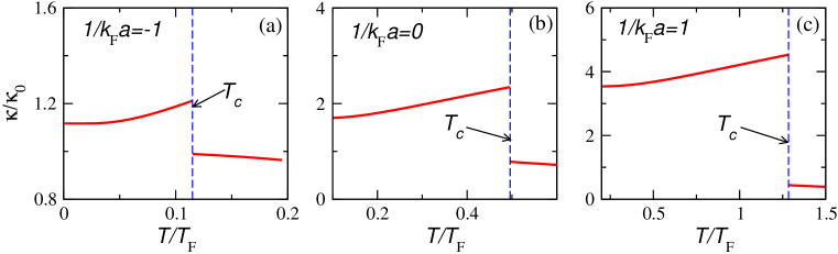
Figure 1: Compressibility at the strict mean field level and as function of temperature from BCS to BEC. $T_{F}$ is the Fermi temperature. $\kappa_{0}=\frac{3}{2}\frac{1}{nE_{F}}$ is the compressibility for a noninteracting Fermi gas at $T=0$.

One of the best measures of a linear response theory is the calculation of the compressibility

$$\kappa=n^{-2}(dn/d\mu)$$

based on the density correlation functions. This is particularly problematic because of the difficulty of finding the same answer as found from thermodynamics. It is of considerable interest, then, to establish the form of the compressibility in a theory with full (compressibility) sum rule compatibility. At the mean field level the behavior above the transition temperature is that of a free Fermi gas. Below $T_{c}$, the compressibility either via thermodynamics or via the two body density density response leads to

$$\frac{\partial n}{\partial\mu}=-K^{00}(0,\mathbf{q}\rightarrow\mathbf{0})$$ (56)

where $K^{00}=Q^{00}_{33}+\delta K^{00}$.

Fig.1 plots the compressibility $\kappa$ as a function of temperature for $1/k_{F}a=-1$ (on the BCS side), $0$ (the unitary point), and $1$ (on the BEC side). The figure exhibits an expected thermodynamic signature of a phase transition, appearing as a discontinuity in the compressibility at $T_{c}$. The discontinuity in $\kappa$ at $T_{c}$ can be traced back to the appearance of collective-mode term $\delta K^{00}$ which sets in below $T_{c}$ and is absent in the normal state. It should be noted that at $T_{c}$, $\delta K^{00}$ is finite only when $\omega=0$. When $\omega$ approaches but does not equal $0$, we have $\delta K^{00}\rightarrow 0$ at $T_{c}$. In this way $\delta K^{00}$ is not analytic at $\omega=0$.

Additional properties of the BCS to BEC crossover can be analyzed similarly. For example, in Appendix B we analytically evaluate the $T=0$ density structure factor in the BCS and BEC limits. Here one sees that at $T=0$ the density structure factor for low frequency and momentum is dominated by the gapless collective mode. As one crosses from BCS to BEC, this mode appears as the usual sound mode of BCS theory and evolves continuously into the Bogoliubov mode and eventually to the free bosonic dispersion in the BEC regime.

One can similarly address the spin response functions following, for example the derivation in Ref. Guo et al. (2013). Importantly, the collective modes appear only in the density response and do not couple to the spin response functions. This supports the discussion given in the introduction that any algebra involving both the density and spin response functions which decomposes these functions into separate $\uparrow$ and $\downarrow$ contributions (see Eq. (2)) is generally problematic, except in the absence of interactions. Such algebraic manipulations are not possible when the diagram sets in different channels are not the same.

V Consistent Linear Response Theory Above $T_{c}$: Example of Pair Correlated State

We now turn to the compressibility in a theory (of the normal phase) which includes pair correlations. It is notable that here too, one finds consistency with the usual Ward (and $Q$-limit Ward) identities, providing one restricts consideration to the theory originally introduced by Nozieres and Schmitt-Rink Nozières and Schmitt-Rink (1985) for the normal phase only. The NSR paper was among the first to emphasize the importance of treating pair correlations in the normal phase. Indeed these were discussed along with an analysis of the ground state considered here and introduced by Leggett Leggett (1980) and Eagles Eagles (1969). Interestingly, theories which incorporate correlated pairs which are based on this NSR scheme do not appear to relate to the BCS-Leggett ground state Levin et al. (2010). This is, in part a reflection of the rather ubiquitous first order transition associated with extending NSR theory below $T_{c}$. Our group Chen et al. (2005) has extensively discussed one approach which appears (rather uniquely) to lead to a second order transition from a different (as compared to NSR) normal phase into this well known ground state. However, it is more complicated than the NSR theory, and the related compressibility will be presented elsewhere.

Here, in order to illustrate a fully consistent approach to linear response in the normal phase (beyond that of a noninteracting Fermi gas) we use the simpler NSR scheme. Even though it has been improved and reviewed many times (see Refs. Pethick and Smith (2008); Ueda (2010) for reviews), a full discussion on the linear response theory within NSR theory is still lacking. In a previous publication Levin et al. (2010) we have shown that by carefully choosing a set of diagrams for the vertex function, the NSR theory respects the usual Ward Identity associated with gauge invariance. Here we will show that the compressibility derived from this vertex function also satisfies the compressibility sum rule.

We begin with a brief review of the NSR theory and its linear response theory. The self energy is $\Sigma(K)=\sum_{Q}t_{0}(Q)G_{0}(Q-K)$ with $t_{0}(Q)=1/[g^{-1}+\chi_{0}(Q)]$ being the $t$-matrix in which $\chi_{0}(Q)=\sum_{P}G_{0}(P)G_{0}(Q-P)$ is the pair susceptibility. The number equation is given by $n=2\sum_{K}G(K)$ while an approximate number equation was implemented in the original NSR paper Nozières and Schmitt-Rink (1985). The response function may also be written formally as

$$K^{\mu\nu}(i\Omega_{l},\mathbf{q})=2\sum_{P}\Gamma^{\mu}(P+Q,P)G(P+Q)\gamma^{\nu}(P,P+Q)G(P)+\frac{n}{m}h^{\mu\nu},$$ (57)

where the full EM vertex function $\Gamma^{\mu}$ must obey the Ward identity (6) so that $q_{\mu}K^{\mu\nu}(Q)=0$. The correction to the full vertex function should be consistent with that of the self energy, hence it is associated with the set of diagrams shown in Fig.2. We have

$$\Gamma^{\mu}(P+Q,P)=\gamma^{\mu}(P+Q,P)+\textrm{MT}^{\mu}(P+Q,P)+\textrm{AL}^{\mu}(P+Q,P),$$ (58)

where we identify the Maki-Thompson (MT) and Aslamazov-Larkin (AL) diagrams with

$$\textrm{MT}^{\mu}(P+Q,P) = \sum_{K}t_{0}(K)G_{0}(K-P)\gamma^{\mu}(K-P,K-P-Q)G_{0}(K-P-Q),$$

$$\textrm{AL}^{\mu}(P+Q,P) = -2\sum_{L,K}t_{0}(K)t_{0}(K+Q)G_{0}(K-P)G_{0}(K-L)G_{0}(L+Q)\gamma^{\mu}(L+Q,L)G_{0}(L).$$

The factor $2$ in the AL diagram comes from the fact that the vertex can be inserted in one of the two fermion propagators in the $t$-matrix and the minus sign is because inserting the vertex splits the t-matrix in the self energy.

To prove that the full vertex in Eq. (58) satisfies the Ward Identity we contract the MT and AL terms with $q_{\mu}$ to yield

$$q_{\mu}\textrm{MT}^{\mu}(P+Q,P) = \sum_{K}t_{0}(K)G_{0}(K-P)[G_{0}^{-1}(K-P)-G_{0}^{-1}(K-P-Q)]G_{0}(K-P-Q),$$ (59)

$$= -[\Sigma(P)-\Sigma(P+Q)].$$

$$q_{\mu}\textrm{AL}^{\mu}(P+Q,P) = -2\sum_{L,K}t_{0}(K)t_{0}(K+Q)G_{0}(K-P)G_{0}(K-L)G_{0}(L+Q)[G_{0}^{-1}(L+Q)-G_{0}^{-1}(L)]G_{0}(L),$$ (60)

$$= 2[\Sigma(P)-\Sigma(P+Q)].$$

In deriving the second relation, the identity $\chi_{0}(K)-\chi_{0}(K+Q)=t_{0}^{-1}(K)-t_{0}^{-1}(K+Q)$ has been applied. One can then show that the Ward identity

$$q_{\mu}\Gamma^{\mu}(P+Q,P)=G^{-1}_{0}(P+Q)-G^{-1}_{0}(P)+\Sigma(P)-\Sigma(P+Q)=G^{-1}(P+Q)-G^{-1}(P)$$ (61)

is satisfied. Thus the linear response theory based on NSR theory with the vertex function shown in Fig.2 is gauge invariant.

Figure 2: The diagrams for the vertex function of NSR theory. The first one on the right hand side is the bare vertex, the second one is the “MT” diagram, and the last one is the “AL” diagram. Hollow and solid dots denote full and bare vertices. Solid lines and wavy lines correspond to propagator of non-interacting fermions and t-matrix, respectively. Due to the two ways of connecting the fermion propagator inside a $t$-matrix, there are two AL diagrams.

Importantly, this same vertex also satisfies the $Q$-limit Ward Identity

$$\lim_{\mathbf{q}\rightarrow\mathbf{0}}\Gamma^{0}(P+Q,P)|_{\omega=0}=1-\frac{\partial\Sigma(P)}{\partial\mu}.$$ (62)

By explicitly calculating the vertex function, we have

$$\lim_{\mathbf{q}\rightarrow\mathbf{0}}\Gamma^{0}(P+Q,P)|_{\omega=0}=1+\sum_{K}t_{0}(K)G^{2}_{0}(K-P)-2\sum_{L,K}t^{2}_{0}(K)G_{0}(K-P)G_{0}(K-L)G^{2}_{0}(L).$$ (63)

Now we evaluate the right hand side of Eq.(62) for NSR theory.

$$1-\frac{\partial\Sigma(P)}{\partial\mu}=1-\left(\sum_{K}\frac{\partial t_{0}(K)}{\partial\mu}G_{0}(K-P)+\sum t_{0}(K)\frac{\partial G_{0}(K-P)}{\partial\mu}\right)$$ (64)

$$= 1-2\sum_{L,K}t^{2}_{0}(K)G_{0}(K-P)G_{0}(K-L)G^{2}_{0}(L)+\sum_{K}t_{0}(K)G^{2}_{0}(K-P)$$

$$= \lim_{\mathbf{q}\rightarrow\mathbf{0}}\Gamma^{0}(P+Q,P)|_{\omega=0},$$

Thus the $Q$-limit WI is satisfied by the linear response theory of the NSR theory. As a consequence, the compressibility sum rule is satisfied by this linear response theory. We emphasize that these two constraints (the $Q$-limit Ward identity (62) and the Ward identity (61)) are independent constraints Guo et al. (2013). These observations should be contrasted with the Hartree-Fock as well as the RPA approximations reviewed in Ref. Mahan (2000) which cannot reach this level of consistency.

Despite these findings, the compressibility is, nevertheless, ill behaved, as it diverges when the system approaches $T_{c}$ from above. This problem was discussed in Ref. Strinati et al. (2002), where it was shown that the MT and AL diagrams diverge as $T\rightarrow T_{c}$. We note that in NSR theory, $T_{c}$ is determined by the temperature where $t_{0}^{-1}(Q=0)=0$ Nozières and Schmitt-Rink (1985), as in the Thouless criterion in conventional superconductors Thouless (1960). In the number equation, the $t$-matrix resides in the denominator of $G(K)$ so its divergence at $T_{c}$ does not introduce difficulties. However, if one calculates $dn/d\mu$ or equivalently calculates the MT and AL diagrams, those expressions explicitly contain $\frac{d\Sigma}{d\mu}$ in the numerator. In NSR theory, we have $\frac{d\Sigma}{d\mu}=-\sum_{q}\frac{d\chi/d\mu}{(1+g\chi)^{2}}G_{0}(q-k)+\cdots$. Due to the Thouless criterion, $1+g\chi\to\,aq^{2}$ for small $q$ when $T\to T_{c}$. Then the $q$ integral behaves like $\int\frac{q^{2}dq}{q^{4}}$ which is divergent at $q=0$.

There have been attempts to remove this divergence by including effective boson-boson interactions Palestini et al. (2012), but there has been no demonstration that gauge invariance and conservation laws are respected Chien et al. (2012) when these repairs are made. One can identify more generally the problematic aspect of NSR theory. In this simplest pairing fluctuation scheme, where the $t$-matrix contains only bare Green’s functions, the fermionic chemical potential $\mu$ is effectively the only parameter in the theory. Once dressed Green’s functions are introduced, it becomes possible to avoid this type of divergence. At the same time, of course, it becomes more difficult to establish consistency with gauge invariance and the compressibility sum rule. Given that the compressibility sum rule is rarely satisfied (the exceptions being the two examples discussed in this paper), one has a choice for how to approach a calculation of the compressibility. We emphasize that from the literature it appears that the more credible results for the compressibility arise Singwi et al. (1968) via the thermodynamic rather than the two body correlation functions.

VI Conclusion

Linear response theories have been an important tool for studying transport and dynamic properties of superfluid and related many-particle systems. The current focus in the literature on ultracold Fermi superfluids, particularly at unitarity, provided a primary motivation for our work which aimed to organize this subject matter and clarify the constraints that calibrate a linear response theory. We have seen that the challenge is to construct such theories as to be fully compatible with $f$-sum and compressibility-sum rules which reflect conservation principles. Although there have been some successes there are nevertheless important failures.

In this paper we presented two nearly unique examples of fermionic superfluids which are demonstrably consistent with $f$-sum and compressibility-sum rules. We addressed these theories via the compressibility $\kappa$. Important here was that both are compatible with the compressibility sum rule. It is useful to compare these two observations in the normal phase. In effect, the BCS-BEC mean field approach treated the normal phase as a normal Fermi liquid and the resulting compressibility is plotted in Figure 1. Above $T_{c}$ one finds very little temperature dependence. This should be contrasted with the behavior found in the Nozieres Schmitt-Rink approach to the normal phase, where there is a dramatic upturn in the compressibility with decreasing temperature. Precisely at $T_{c}$ the NSR theory predicts that $\kappa$ diverges Strinati et al. (2002).

One can view the first of these two systems as indicating the behavior of $\kappa$ associated with a purely fermionic system. By contrast the dramatic upturn in $\kappa$ with decreasing $T$ is expected for a bosonic system en route to condensation. Experimentally Ku et al. (2012) the situation for unitary gases is somewhat in between these two limits. This will be an important topic for future research.

Hao Guo thanks the support by National Natural Science Foundation of China (Grants No. 11204032) and Natural Science Foundation of Jiangsu Province, China (SBK201241926). C. C. C. acknowledges the support of the U.S. Department of Energy through the LANL/LDRD Program. Additional support (KL) is via NSF-MRSEC Grant 0820054.

Appendix A Detailed expressions for response functions

The following are the EM response functions of fermionic superfluids from the CFOP theory:

$$Q_{11}(\omega,\mathbf{q}) = \sum_{\mathbf{p}}\Big{[}\big{(}1+\frac{\xi^{+}_{\mathbf{p}}\xi^{-}_{\mathbf{p}}-\Delta^{2}}{E^{+}_{\mathbf{p}}E^{-}_{\mathbf{p}}}\big{)}\frac{E^{+}_{\mathbf{p}}+E^{-}_{\mathbf{p}}}{\omega^{2}-(E^{+}_{\mathbf{p}}+E^{-}_{\mathbf{p}})^{2}}[1-f(E^{+}_{\mathbf{p}})-f(E^{-}_{\mathbf{p}})]$$ (65)

$$\quad-\big{(}1-\frac{\xi^{+}_{\mathbf{p}}\xi^{-}_{\mathbf{p}}-\Delta^{2}}{E^{+}_{\mathbf{p}}E^{-}_{\mathbf{p}}}\big{)}\frac{E^{+}_{\mathbf{p}}-E^{-}_{\mathbf{p}}}{\omega^{2}-(E^{+}_{\mathbf{p}}-E^{-}_{\mathbf{p}})^{2}}[f(E^{+}_{\mathbf{p}})-f(E^{-}_{\mathbf{p}})]\Big{]},$$

$$Q_{12}(\omega,\mathbf{q})=-Q_{21}(\omega,\mathbf{q})=-i\omega\sum_{\mathbf{p}}\Big{[}\big{(}\frac{\xi^{+}_{\mathbf{p}}}{E^{+}_{\mathbf{p}}}+\frac{\xi^{-}_{\mathbf{p}}}{E^{-}_{\mathbf{p}}}\big{)}\frac{1-f(E^{+}_{\mathbf{p}})-f(E^{-}_{\mathbf{p}})}{\omega^{2}-(E^{+}_{\mathbf{p}}+E^{-}_{\mathbf{p}})^{2}}-\big{(}\frac{\xi^{+}_{\mathbf{p}}}{E^{+}_{\mathbf{p}}}-\frac{\xi^{-}_{\mathbf{p}}}{E^{-}_{\mathbf{p}}}\big{)}\frac{f(E^{+}_{\mathbf{p}})-f(E^{-}_{\mathbf{p}})}{\omega^{2}-(E^{+}_{\mathbf{p}}-E^{-}_{\mathbf{p}})^{2}}\Big{]},$$ (66)

$$Q^{0}_{13}(\omega,\mathbf{q})=Q^{0}_{31}(\omega,\mathbf{q})=\Delta\sum_{\mathbf{p}}\frac{\xi^{+}_{\mathbf{p}}+\xi^{-}_{\mathbf{p}}}{E^{+}_{\mathbf{p}}E^{-}_{\mathbf{p}}}\Big{[}\frac{(E^{+}_{\mathbf{p}}+E^{-}_{\mathbf{p}})[1-f(E^{+}_{\mathbf{p}})-f(E^{-}_{\mathbf{p}})]}{\omega^{2}-(E^{+}_{\mathbf{p}}+E^{-}_{\mathbf{p}})^{2}}+\frac{(E^{+}_{\mathbf{p}}-E^{-}_{\mathbf{p}})[f(E^{+}_{\mathbf{p}})-f(E^{-}_{\mathbf{p}})]}{\omega^{2}-(E^{+}_{\mathbf{p}}-E^{-}_{\mathbf{p}})^{2}}\Big{]},$$ (67)

$$\mathbf{Q}^{i}_{13}(\omega,\mathbf{q})=\mathbf{Q}_{31}^{i}(\omega,\mathbf{q})=\sum_{\mathbf{p}}\frac{\mathbf{p}^{i}}{m}\frac{\Delta\omega}{E^{+}_{\mathbf{p}}E^{-}_{\mathbf{p}}}\Big{[}\frac{(E^{+}_{\mathbf{p}}-E^{-}_{\mathbf{p}})[1-f(E^{+}_{\mathbf{p}})-f(E^{-}_{\mathbf{p}})]}{\omega^{2}-(E^{+}_{\mathbf{p}}+E^{-}_{\mathbf{p}})^{2}}+\frac{(E^{+}_{\mathbf{p}}+E^{-}_{\mathbf{p}})[f(E^{+}_{\mathbf{p}})-f(E^{-}_{\mathbf{p}})]}{\omega^{2}-(E^{+}_{\mathbf{p}}-E^{-}_{\mathbf{p}})^{2}}\Big{]},$$ (68)

$$Q_{22}(\omega,\mathbf{q}) = \sum_{\mathbf{p}}\Big{[}\big{(}1+\frac{\xi^{+}_{\mathbf{p}}\xi^{-}_{\mathbf{p}}+\Delta^{2}}{E^{+}_{\mathbf{p}}E^{-}_{\mathbf{p}}}\big{)}\frac{E^{+}_{\mathbf{p}}+E^{-}_{\mathbf{p}}}{\omega^{2}-(E^{+}_{\mathbf{p}}+E^{-}_{\mathbf{p}})^{2}}[1-f(E^{+}_{\mathbf{p}})-f(E^{-}_{\mathbf{p}})]$$ (69)

$$\quad-\big{(}1-\frac{\xi^{+}_{\mathbf{p}}\xi^{-}_{\mathbf{p}}+\Delta^{2}}{E^{+}_{\mathbf{p}}E^{-}_{\mathbf{p}}}\big{)}\frac{E^{+}_{\mathbf{p}}-E^{-}_{\mathbf{p}}}{\omega^{2}-(E^{+}_{\mathbf{p}}-E^{-}_{\mathbf{p}})^{2}}[f(E^{+}_{\mathbf{p}})-f(E^{-}_{\mathbf{p}})]\Big{]},$$

$$Q^{0}_{23}(\omega,\mathbf{q})=-Q^{0}_{32}(\omega,\mathbf{q})=i\sum_{\mathbf{p}}\frac{\Delta\omega}{E^{+}_{\mathbf{p}}E^{-}_{\mathbf{p}}}\Big{[}\frac{(E^{+}_{\mathbf{p}}+E^{-}_{\mathbf{p}})[1-f(E^{+}_{\mathbf{p}})-f(E^{-}_{\mathbf{p}})]}{\omega^{2}-(E^{+}_{\mathbf{p}}+E^{-}_{\mathbf{p}})^{2}}+\frac{(E^{+}_{\mathbf{p}}-E^{-}_{\mathbf{p}})[f(E^{+}_{\mathbf{p}})-f(E^{-}_{\mathbf{p}})]}{\omega^{2}-(E^{+}_{\mathbf{p}}-E^{-}_{\mathbf{p}})^{2}}\Big{]},$$ (70)

$$\mathbf{Q}^{i}_{23}(\omega,\mathbf{q})=-\mathbf{Q}^{i}_{32}(\omega,\mathbf{q})=i\Delta\sum_{\mathbf{p}}\frac{\mathbf{p}^{i}}{m}\frac{\xi^{+}_{\mathbf{p}}-\xi^{-}_{\mathbf{p}}}{E^{+}_{\mathbf{p}}E^{-}_{\mathbf{p}}}\Big{[}\frac{(E^{+}_{\mathbf{p}}+E^{-}_{\mathbf{p}})[1-f(E^{+}_{\mathbf{p}})-f(E^{-}_{\mathbf{p}})]}{\omega^{2}-(E^{+}_{\mathbf{p}}+E^{-}_{\mathbf{p}})^{2}}+\frac{(E^{+}_{\mathbf{p}}-E^{-}_{\mathbf{p}})[f(E^{+}_{\mathbf{p}})-f(E^{-}_{\mathbf{p}})]}{\omega^{2}-(E^{+}_{\mathbf{p}}-E^{-}_{\mathbf{p}})^{2}}\Big{]},$$ (71)

$$Q_{33}^{00}(\omega,\mathbf{q}) = \sum_{\mathbf{p}}\Big{[}\big{(}1-\frac{\xi^{+}_{\mathbf{p}}\xi^{-}_{\mathbf{p}}-\Delta^{2}}{E^{+}_{\mathbf{p}}E^{-}_{\mathbf{p}}}\big{)}\frac{E^{+}_{\mathbf{p}}+E^{-}_{\mathbf{p}}}{\omega^{2}-(E^{+}_{\mathbf{p}}+E^{-}_{\mathbf{p}})^{2}}[1-f(E^{+}_{\mathbf{p}})-f(E^{-}_{\mathbf{p}})]$$ (72)

$$\quad-\big{(}1+\frac{\xi^{+}_{\mathbf{p}}\xi^{-}_{\mathbf{p}}-\Delta^{2}}{E^{+}_{\mathbf{p}}E^{-}_{\mathbf{p}}}\big{)}\frac{E^{+}_{\mathbf{p}}-E^{-}_{\mathbf{p}}}{\omega^{2}-(E^{+}_{\mathbf{p}}-E^{-}_{\mathbf{p}})^{2}}[f(E^{+}_{\mathbf{p}})-f(E^{-}_{\mathbf{p}})]\Big{]}.$$

$$\tensor{Q}_{33}^{ij}(\omega,\mathbf{q}) = \sum_{\mathbf{p}}\frac{\mathbf{p}^{i}\mathbf{p}^{j}}{m^{2}}\Big{[}\big{(}1-\frac{\xi^{+}_{\mathbf{p}}\xi^{-}_{\mathbf{p}}+\Delta^{2}}{E^{+}_{\mathbf{p}}E^{-}_{\mathbf{p}}}\big{)}\frac{E^{+}_{\mathbf{p}}+E^{-}_{\mathbf{p}}}{\omega^{2}-(E^{+}_{\mathbf{p}}+E^{-}_{\mathbf{p}})^{2}}[1-f(E^{+}_{\mathbf{p}})-f(E^{-}_{\mathbf{p}})]$$ (73)

$$\qquad\quad-\big{(}1+\frac{\xi^{+}_{\mathbf{p}}\xi^{-}_{\mathbf{p}}+\Delta^{2}}{E^{+}_{\mathbf{p}}E^{-}_{\mathbf{p}}}\big{)}\frac{E^{+}_{\mathbf{p}}-E^{-}_{\mathbf{p}}}{\omega^{2}-(E^{+}_{\mathbf{p}}-E^{-}_{\mathbf{p}})^{2}}[f(E^{+}_{\mathbf{p}})-f(E^{-}_{\mathbf{p}})]\Big{]},$$

$$\mathbf{Q}^{0i}_{33}(\omega,\mathbf{q})=\mathbf{Q}^{i0}_{33}(\omega,\mathbf{q})=\omega\sum_{\mathbf{p}}\frac{\mathbf{p}^{i}}{m}\Big{[}\big{(}\frac{\xi^{+}_{\mathbf{p}}}{E^{+}_{\mathbf{p}}}-\frac{\xi^{-}_{\mathbf{p}}}{E^{-}_{\mathbf{p}}}\big{)}\frac{1-f(E^{+}_{\mathbf{p}})-f(E^{-}_{\mathbf{p}})}{\omega^{2}-(E^{+}_{\mathbf{p}}+E^{-}_{\mathbf{p}})^{2}}-\big{(}\frac{\xi^{+}_{\mathbf{p}}}{E^{+}_{\mathbf{p}}}+\frac{\xi^{-}_{\mathbf{p}}}{E^{-}_{\mathbf{p}}}\big{)}\frac{f(E^{+}_{\mathbf{p}})-f(E^{-}_{\mathbf{p}})}{\omega^{2}-(E^{+}_{\mathbf{p}}-E^{-}_{\mathbf{p}})^{2}}\Big{]}.$$ (74)

Appendix B Density Structure Factor in the BCS and BEC limits

We first consider the BCS limit and the regime where the external frequency and momentum are small, such that $0<\omega<2\Delta$ and $0<q\ll k_{F}$. Due to the particle-hole symmetry of strict BCS theory, $Q_{12}=Q^{0}_{13}=0$ so $K^{00}=K^{00}_{0}+\delta K^{00}$, where $K^{00}_{0}=Q^{00}_{33}$ and $\delta K^{00}=-Q^{0}_{23}Q^{0}_{32}/\tilde{Q}_{22}$. The density structure factor is $\chi_{\rho\rho}=\chi_{\rho\rho 0}+\delta\chi_{\rho\rho}$, where $\chi_{\rho\rho 0}=-\frac{1}{\pi}\textrm{Im}K^{00}_{0}$ and $\delta\chi_{\rho\rho 0}=-\frac{1}{\pi}\textrm{Im}\delta K^{00}$ according to Eq.(31).

Our small frequency and small momentum limit guarantees that it is not possible to break a Cooper pair into two quasi-particles. Therefore $\chi_{\rho\rho 0}$ has no pole. Instead, $\tilde{Q}_{22}$ determines the poles of $\chi_{\rho\rho}$. This leads to

$$\tilde{Q}_{22}(\omega,\mathbf{q})=-\frac{N(0)}{2\Delta^{2}}\big{(}\omega^{2}-c^{2}_{s}q^{2}\big{)}.$$ (75)

Here $N(0)$ is the density of states at the Fermi energy. The condition $\tilde{Q}_{22}=0$ yields the excitation dispersion of the gapless mode $\omega=c_{s}q$, where $c_{s}=\frac{1}{\sqrt{3}}\frac{k_{F}}{m}$. Similarly, we have

$$Q^{0}_{23}(\omega,\mathbf{q})\simeq-\frac{i\Delta\omega N(0)}{2}\int^{+\infty}_{-\infty}d\xi_{\mathbf{p}}\frac{1}{E^{3}_{\mathbf{p}}}=-\frac{i\omega N(0)}{\Delta}.$$ (76)

One then finds for the density structure factor in the BCS limit

$$\chi_{\rho\rho}(\omega,\mathbf{q})=-\frac{\omega^{2}N(0)}{c_{s}q\pi}\textrm{Im}\Big{(}\frac{1}{\omega-c_{s}q+i\delta}-\frac{1}{\omega+c_{s}q+i\delta}\Big{)}=\frac{nq}{2mc_{s}}\delta(\omega-c_{s}q),$$ (77)

which also satisfies the $f$-sum rule

$$\int^{\infty}_{0}d\omega\omega\chi_{\rho\rho}(\omega,\mathbf{q})=n\frac{q^{2}}{2m}.$$ (78)

Next we evaluate the density-density correlation functions in the BEC limit for different $\omega,q$ regimes. We consider three situations associated with (A) $\frac{\Delta}{|\mu|}\rightarrow 0$ and low frequency and momentum, (B) $\frac{\Delta}{|\mu|}<1$ and low frequency and momentum, and (C) $q^{2}/2m+|\mu|\gg\Delta$ respectively. Case (A) describes the deep BEC limit where $a\rightarrow 0^{+}$ and $\Delta/|\mu|\rightarrow 0$. Here low momentum implies $q\ll k_{F}$ as before while low frequency means $\omega\ll\Delta_{\textrm{S}}=2\sqrt{|\mu|^{2}+\Delta^{2}}$, where $\Delta_{\textrm{S}}$ is the threshold for fermionic excitations in the BEC regime. Case (B) corresponds to a relatively shallow BEC regime as compared to Case (A). In Case (C), when $q$ is sufficiently large, the system is in the very shallow BEC regime where $\mu\rightarrow 0$ at $1/k_{F}a=0.553$. This situation was discussed in Ref.Combescot et al. (2006b). The evaluation of the structure factor is lengthy, but straightforward.

(A). In this case, the system is in the deep BEC limit and can be thought as a dilute gas of tightly bound molecules with mass $m_{B}=2m$. Hence, the gap $\Delta$ is negligible and we may approximate $E^{\pm}_{\mathbf{p}}\simeq\xi^{\pm}_{\mathbf{p}}$ and $\tilde{Q}_{11}\simeq\tilde{Q}_{22}$. Here one finds that

$$\chi_{\rho\rho}(\omega,\mathbf{q})=\frac{2\Delta^{2}(2m)^{\frac{3}{2}}\sqrt{|\mu|}}{\pi}\frac{2m}{q^{2}}\mbox{Arcsin}^{2}\frac{\frac{q}{\sqrt{2m}}}{\sqrt{\frac{q^{2}}{2m}+16|\mu|}}\delta(\omega-\frac{q^{2}}{4m}).$$ (79)

Note that $\omega=\frac{q^{2}}{4m}=\frac{q^{2}}{2m_{B}}$ appears as an argument in the delta function, corresponding to the energy dispersion of free bosons with mass $m_{B}=2m$. We note that the fermionic continuum (associated with broken pairs) does not appear at these low $\omega$.

(B). In this case, the system behaves as a weakly interacting Bose gas where the internal structure of the fermion pairs can not be ignored. We expand all response functions to leading order in $\Delta$, $q^{2}/2m$ and $\omega$ and assume $E^{\pm}_{\mathbf{p}}\simeq\xi^{\pm}_{\mathbf{p}}$ with $\tilde{Q}_{11}\neq\tilde{Q}_{22}$. The density structure factor is given by

$$\chi_{\rho\rho}(\omega,\mathbf{q})=2n\frac{\frac{q^{2}}{4m}-\frac{\omega^{2}_{s}}{8|\mu|}}{\omega_{s}}\delta(\omega-\omega_{s}),$$ (80)

where $\omega_{s}=\sqrt{c^{2}_{s}q^{2}+(\frac{q^{2}}{4m})^{2}}$ is the dispersion of the Bogoliugov mode.

(C). Since $\Delta\ll q^{2}/2m+|\mu|$, we expand the energy dispersion relation to leading order in $\Delta$ as $E^{\pm}_{\mathbf{p}}=\xi^{\pm}_{\mathbf{p}}+\Delta^{2}/2\xi^{\pm}_{\mathbf{p}}$(Combescot et al., 2006b). If, in addition, the system is in the regime $\frac{\Delta}{|\mu|}<1$, we may expand the density structure factor to first order in $\Delta^{2}/|\mu|^{2}$ to obtain

$$\chi_{\rho\rho}(\omega,\mathbf{q})=2n\big{[}1-\frac{5}{16}\frac{\Delta^{2}}{|\mu|^{2}}-(\frac{1}{24}-\frac{17}{256}\frac{\Delta^{2}}{|\mu|^{2}})\frac{q^{2}}{2m|\mu|}+\cdots\big{]}\delta(\omega-\omega_{c}).$$ (81)

References

- Ueda (2010) M. Ueda, Fundamentals and new frontiers of Bose-Einstein condensation (World scientific, Singapore, 2010).
- Guo et al. (2013) H. Guo, C. C. Chien, and Y. He, J. Low Temp. Phys. 172, 5 (2013).
- Levin et al. (2010) K. Levin, Q. J. Chen, C. C. Chien, and Y. He, Ann. Phys. 325, 233 (2010).
- Nozières and Schmitt-Rink (1985) P. Nozières and S. Schmitt-Rink, J. Low Temp. Phys. 59, 195 (1985).
- Mahan (2000) G. D. Mahan, Many-Particle Physics (Kluwer academic/Plenum publishers, New York, 2000), 3rd ed.
- Singwi et al. (1968) K. S. Singwi, M. P. Tosi, R. H. Land, and A. Sjolander, Phys. Rev. 176, 589 (1968).
- He et al. (1994) S. He, S. H. Simon, and B. I. Halperin, Phys. Rev. B 50, 1823 (1994).
- Nambu (1960) Y. Nambu, Phys. Rev. 117, 648 (1960).
- Kadanoff and Martin (1961) L. P. Kadanoff and P. C. Martin, Phys. Rev. 124, 670 (1961).
- Betbeder Matibet and Nozieres (1969) O. Betbeder Matibet and P. Nozieres, Ann. Phys. (NY) 51, 392 (1969).
- Stephen (1963) M. J. Stephen, Phys. Rev. 139, A197 (1963).
- Yu et al. (2009) Z. Yu, G. M. Bruun, and G. Baym, Phys. Rev. A 80, 023615 (2009).
- Wolfe and Volhardt (1990) P. Wolfe and D. Volhardt, The Superfluid Phases of Helium 3 (Taylor and Francis, Oxford, UK, 1990).
- Kubo et al. (2004) R. Kubo, M. Toda, and N. Hashitsume, Statistical Physics II: Nonequilibrium Statistical Mechanics (Springer-Verlag, 2004), 2nd ed.
- Combescot et al. (2006a) R. Combescot, P. Giorgini, and S. Stringari, Eur. Phys. Lett 75, 695 (2006a).
- Hu et al. (2010) H. Hu, X. J. Liu, P. Dyke, M. Mark, P. D. Drummond, P. Hannaford, and C. J. Vale, Phys. Rev. Lett. 105, 070402 (2010).
- Mihaila et al. (2005) B. Mihaila, S. Gaudio, K. B. Blagoev, A. V. Balatsky, P. B. Littlewood, and D. L. Smith, Phys. Rev. Lett. 95, 090402 (2005).
- Son and Thompson (2010) D. T. Son and E. G. Thompson, Phys. Rev. A 81, 063634 (2010).
- Yoshimi et al. (2009) K. Yoshimi, T. Kato, and H. Maebashi, J. Phys. Soc. Jpn. 78, 104002 (2009).
- Schrieffer (1964) J. R. Schrieffer, Theory of superconductivity (Benjamin, New York, 1964).
- Fetter and Walecka (2003) A. L. Fetter and J. D. Walecka, Quantum Theory of Many-Particle Systems (Dover Publications, New York, 2003).
- Benfatto et al. (2004) L. Benfatto, A. Toschi, and S. Caprara, Phys. Rev. B 69, 184510 (2004).
- Combescot et al. (2006b) R. Combescot, M. Y. Kagan, and S. Stringari, Phys. Rev. A 74, 042717 (2006b).
- Chen et al. (2005) Q. J. Chen, J. Stajic, S. N. Tan, and K. Levin, Phys. Rep. 412, 1 (2005).
- Leggett (1980) A. J. Leggett, in Modern Trends in the Theory of Condensed Matter (Springer-Verlag, Berlin, 1980), pp. 13–27.
- Mihaila et al. (2011) B. Mihaila, J. F. Dawson, F. Cooper, C. C. Chien, and E. Timmermans, Phys. Rev. A 83, 053637 (2011).
- Eagles (1969) D. M. Eagles, Phys. Rev. 186, 456 (1969).
- Pethick and Smith (2008) C. J. Pethick and H. Smith, Bose-Einstein Condensation in Dilute Gases (Cambridge University Press, Cambridge, 2008), 2nd ed.
- Strinati et al. (2002) G. C. Strinati, P. Pieri, and C. Lucheroni, Eur. Phys. J. B 30, 161 (2002).
- Thouless (1960) D. J. Thouless, Ann. Phys. 10, 553 (1960).
- Palestini et al. (2012) F. Palestini, P. Pieri, and G. C. Strinati, Phys. Rev. Lett. 108, 080401 (2012).
- Chien et al. (2012) C. C. Chien, H. Guo, and K. Levin, Phys. Rev. Lett. 109, 118901 (2012).
- Ku et al. (2012) M. J. H. Ku, A. T. Sommer, L. W. Cheuk, and M. W. Zwierlein, Science 335, 563 (2012).