Numerical modelling of the lobes of radio galaxies in cluster environments

Abstract

We have carried out two-dimensional, axisymmetric, hydrodynamic numerical modelling of the evolution of radio galaxy lobes. The emphasis of our work is on including realistic hot-gas environments in the simulations and on establishing what properties of the resulting radio lobes are independent of the choice of environmental properties and of other features of the models such as the initial jet Mach number. The simulated jet power we use is chosen so that we expect the inner parts of the lobes to come into pressure balance with the external medium on large scales; we show that this leads to the expected departure from self-similarity and the formation of characteristic central structures in the hot external medium. The work done by the expanding radio lobes on the external hot gas is roughly equal to the energy stored in the lobes for all our simulations once the lobes are well established. We show that the external pressure at the lobe midpoint is a reasonable estimate of the internal (lobe) pressure, with only a weak dependence on the environmental parameters: on the other hand, the predicted radio emission from a source of a given physical size has a comparatively strong dependence on the environment in which the lobe resides, introducing an order of magnitude of scatter into the jet power versus radio luminosity relationship. X-ray surface brightness and temperature visualizations of our simulations bear a striking resemblance to observations of some well-studied radio galaxies.

1 Introduction

Ever since the establishment of the standard (‘beam’) model for powerful double radio sources (Scheuer, 1974; Blandford & Rees, 1974) it has been clear that their dynamics must depend strongly on their environment. Scheuer (1974) proposed two limiting cases. In his model A, the transverse expansion of the radio galaxy ignores the external medium; this would be true in practise if radio galaxies were strongly overpressured with respect to their external medium at all times in their lifetime, in which case the lobe pressure would drive a supersonic transverse expansion and we would expect to see an elliptical bow shock surrounding the sources at all times. In model C, on the other hand, the pressure in the lobes becomes comparable to the external pressure, and then, as Scheuer put it, “the outer parts of the cavity swell at the expense of the parts nearest the massive nucleus, where the thermal gas pressure is higher”. Such a model, as Scheuer realised, is significantly harder to deal with analytically.

For this reason popular analytic models of radio lobe dynamics have tended to be descendants of Scheuer’s model A. Begelman & Cioffi (1989) showed that it was possible to construct self-consistent models in which the lobes remained overpressured, and therefore supersonically expanding, throughout a significant part of their lifetimes, while allowing the jet to be confined by the material inside the cocoon. Models of this sort also provide the basis for the important and widely used work of Kaiser & Alexander (1997) (hereafter KA) who constructed an analytic model for the growth of a radio source in a power-law atmosphere using the assumption of self-similar expansion, which restricts the applicability of the model of the model to the strongly overpressured phase. More recently, Hardcastle & Worrall (2000) showed that the minimum pressures in radio lobes were typically comparable to, or less than, the external thermal pressures in the centres of the host groups or clusters, and argued that the KA model, applied to observed extended 3CRR classical double (Fanaroff & Riley 1974 class II, hereafter FRII) sources in group or cluster environments, required much lower cluster temperatures for self-consistency than are actually plausible. Since then, the routine use of X-ray inverse-Compton pressure measurements combined with the information provided by X-ray observations on the external medium (e.g. Hardcastle et al., 2002a; Croston et al., 2004) have shown that our best estimates of the lobe pressures are comparable to the external pressure on scales comparable to those of the midpoints of the lobes, and therefore in general significantly less than the pressure at the centre of the cluster or group environment; either these best estimates of pressure are wrong (for example, because the contributions of non-radiating particles to the lobe pressure has been severely underestimated), or lobes are not strongly overpressured with respect to their environments, and models such as those of KA cannot consistently describe them on the largest scales. Analytical calculations of the structure of FRII radio sources approaching pressure equilibrium have been presented by Alexander (2002); these show that in atmospheres in which pressure/density decreases steeply with radius, a dense layer of ambient gas is predicted next to the radio lobes. Its gravity squeezes the lobes and causes the onset of non-self-similar evolution.

While analytical work is enlightening regarding the general structure and basic physics of those sources, it relies on many assumptions, e.g. about the geometry of the sources. Numerical modelling, in principle, frees us of the limiting assumptions of analytic models and allows us to model radio galaxies whose behaviour is in better agreement with observation. However, the high-resolution simulations required, with their large demands on simulation time, have typically required some compromises. Early numerical modelling (e.g. Norman et al., 1982; Kössl & Müller, 1988; Lind et al., 1989) assumed a uniform-density environment, which is quite possibly not a bad assumption for the early phases of a radio galaxy’s growth but certainly not valid on scales of tens to hundreds of kpc. This was followed by 2D and 3D hydrodynamical modelling of sources in semi-realistic ($\beta$-model) environments (e.g. Reynolds et al., 2002; Basson & Alexander, 2003; Zanni et al., 2003; Krause, 2005). These generally showed deviations from self-similarity in the sense that the axial ratios of the simulated sources did not remain constant, but instead grew with time. More recently, Gaibler, Krause, & Camenzind (2009) have demonstrated in a magnetized jet simulation that self-similarity breaks down when a radio source gets close to pressure equilibrium. Qualitatively, similar results are seen in other MHD simulations with realistic environments (e.g. O’Neill et al., 2005; O’Neill & Jones, 2010); environments derived from simulations of dynamically active clusters are used (e.g. Heinz et al., 2006) and the culmination of this type of work is represented by, for example, Mendygral, Jones, & Dolag (2012) whose simulations are fully 3D, contain magnetic fields, take account of electron transport and loss processes, and embed the radio galaxy in an environment that is itself extracted from a cosmological simulation. Because of the limitations in CPU time, though, the vast majority of the work carried out in this area has involved small numbers of simulations considering one or at most a few different environments. It is thus difficult to get an overview of the effects that the known range of environments, even simply considering such basic properties as scale lengths and large-radius power-law indices, has on the dynamics of the radio sources.

Comparison between analytical and numerical work has also given rise to some puzzling results. As noted above, KA presented convincing physical arguments for the existence of a self-similar expansion law in the overpressured phase. Yet this self-similar expansion is not easily seen in simulations (e.g. Carvalho & O’Dea, 2002). This difficulty is related to the fact that simulations often use a jet that is already collimated as a boundary condition to the simulation. But, as KA showed, the self-similar expansion phase is linked in a crucial way to the self-collimation of the jet by the overpressured lobes (compare also model B of Scheuer 1974). Thus, if a jet is injected into a computational domain in a parallel, collimated way, the jet radius cannot adapt in the proper way, which results in an expansion law that is in detail unphysical. For FRII jet simulations, Komissarov & Falle (1998) have shown that a self-similar scaling is indeed achieved if the jet is injected conically. They were even able to account in detail for the shock structure observed in the Cygnus A jet, produced by the self-collimation, albeit with a worryingly large initial opening angle. Krause et al. (2012) have re-analysed the problem using similar simulations, and found that the problem was related to a matter of definitions: when the same definitions are applied to simulations and observations, they are entirely consistent. In the present paper, we aim to set up FRII radio sources where the jet is self-collimated, so that self-similar expansion is in principle possible, and then to investigate their behaviour when they come into pressure equilibrium.

The desire to know exactly how radio galaxies evolve in realistic environments is not a purely abstract one. Radio galaxies in general provide a unique way to couple the high power of an active nucleus (AGN) to its environment on scales of hundreds of kpc to Mpc, where the effects of AGN radiation are expected to be negligible. They therefore play an important role in models of galaxy formation and evolution, where they provide so-called ‘feedback’, helping to prevent the cooling of large-scale gas and the consequent growth of the host galaxies (e.g. Croton et al., 2006). However, whether the physics of radio galaxies is consistent with the role they are required to play in these models is still an open question (see e.g. McNamara & Nulsen, 2012, for a recent review). For example, it is not remotely clear whether the low-power, Fanaroff-Riley class I (FRI) radio galaxies with extended twin jets, seen in many rich group and poor cluster environments, are having any significant energetic impact on the gas with short cooling times, which exists on scales of a few kpc from the nucleus (e.g. Hardcastle et al., 2002b; Jetha et al., 2007). Such systems are very difficult to model in detail numerically (though see, e.g., the work of Perucho & Martí 2007). Classical double radio galaxies, although rarer, are important in this context simply because they are required to have a strong effect on the external medium through the driving of strong shocks, which increases the entropy of the external medium and offsets cooling, and does so through a comparatively large volume of the environment (much larger than the observed radio lobes); they are also simpler to model. Indeed, some of the early work on numerical modelling with realistic environments (e.g. Basson & Alexander, 2003; Krause, 2005; Zanni et al., 2005; O’Neill et al., 2005) was done with the explicit aim of addressing questions about the energetic effects of a powerful radio source. In this context, Zanni et al. (2005) have shown that energy input by jets may reconcile cluster atmospheres from cosmological simulations with observed X-ray scaling relations for groups and clusters of galaxies. However, again, the small numbers of simulations carried out in these studies mean that it is hard to get an overview of the differences in energy transfer efficiency, if any, that might be expected for different environments. Consequently observers, rather than making use of the results of numerical modelling, have a tendency to use naive estimates of the work done on the external medium (e.g. $p{\rm d}V$ for some pressure $p$) together with estimates of the jet power based on analytical rather than numerical work.

In the present paper we try to address these disconnections between numerical modelling and observation. We use the very large amount of computational power that has become available over the course of the past decade, not to include still more physics in a simulation of an individual radio galaxy, but to carry out simple (though high-resolution and large-volume) simulations of radio galaxies in a wide range of environments. Our objective in doing so is to draw conclusions about the dynamics and energetic input of radio galaxies that may be generally applicable, and to test the validity of some assumptions commonly used by observers.

2 The simulation setup

Our modelling in this paper uses the freely available code PLUTO, version 3.1.1, described by Mignone et al. (2007). We chose to use PLUTO because of its good handling of high Mach number flows and the simplicity with which new problems can be defined. In particular, we employed Pluto’s ‘two-shock’, exact Riemann solver, third order interpolation with the van Leer flux limiter and third-order Runge-Kutta time-stepping. The global accuracy of the method is, however, second order due to the way the fluxes are calculated.

Our general approach follows that of Krause et al. (2012); that is, we inject two, oppositely directed, initially conical flows with high Mach number at the centre of the simulation, and allow them to recollimate in the external pressure. In a uniform-density environment, we would expect this recollimation to take place on a physical scale comparable to the inner scale defined by Alexander (2006),

$$L_{1}=2\sqrt{2}\left(\frac{Q_{0}}{\rho_{x}v_{j}^{3}}\right)^{1/2}$$

where $Q_{0}$ is the jet power, $\rho_{x}$ the external density and $v_{j}$ the jet speed. In such an environment, we would also expect the lobes to come into pressure balance on scales comparable to (Komissarov & Falle, 1998)

$$L_{2}=\left(\frac{Q_{0}}{\rho_{x}c_{x}^{3}}\right)^{1/2}$$

where $c_{x}$ is the external sound speed. As $L_{2}/L_{1}=({\cal M}/2)^{3/2}$, where $\cal M$ is the Mach number of the jet, it is immediately clear that high-resolution simulations are necessary to model high-Mach-number (and therefore realistic) jets out to the scale on which the lobes are likely to come close to pressure equilibrium; the cell size of the simulation needs to be $\ll L_{1}$ and the outer radius of the simulation needs to be of order a few times $L_{2}$. For this reason, we chose to reduce the complexity of the problem by carrying out 2D (except as described below), axisymmetric, hydrodynamic simulations. The co-ordinates are spherical polars and the jets are implemented as a boundary condition at the inner radius, injecting a conical flow with opening angle of 15^∘ [chosen to ensure FRII-like structure: see Krause et al. (2012) for a discussion of the effect of opening angle on the lobe morphology]; that is, at $r=r_{\rm inner}$, for all points with $\theta\leq 15^{\circ}$ or $\theta\geq 345^{\circ}$, we set $\rho=\rho_{0}$, $v_{r}={\cal M}c_{s}$, $v_{\theta}=0$, while for all other values of $\theta$ we use a reflection boundary condition at $r_{\rm inner}$.. A conserved tracer quantity is injected with the jets and we use non-zero values of this quantity to define the lobes in the simulations, as described in more detail below.

An important feature of our modelling is that the environments are not uniform. Instead, we represent the environment by a standard isothermal $\beta$ model (King profile),

$$n=n_{0}\left[1+\left(\frac{r}{r_{\rm c}}\right)^{2}\right]^{-3\beta/2}$$

This introduces a new scale, $r_{\rm c}$ (the core radius) into the problem, meaning that self-similar analytic approaches (e.g. KA) are no longer applicable, but it allows us to represent a range of realistic environments from groups to clusters of galaxies. We impose a gravitational potential, as described by Krause (2005), to stabilize the $\beta$-model atmosphere.

Within the simulations, we take the unit of length to be $L_{1}$, the unit of density to be $\rho_{0}=n_{0}\mu m_{p}$, where $\mu$ is the mean mass per particle, and the unit of speed to be $c_{s}$, the speed of sound in the undisturbed ambient medium. In these units, the central pressure $p_{0}$ is $1/\gamma$, or 3/5. In order to choose sensible values for $r_{\rm c}$ in these units, we need to decide on an external calibration for these quantities. Since our interest is in low-power FRII radio galaxies in rich group/poor cluster environments, we adopt $Q=10^{38}$ W ($10^{45}$ erg s^-1), a plausible value for a low-power FRII jet (e.g. Daly et al., 2012). For the basic environmental properties we use $kT=2$ keV, and $n_{0}=3\times 10^{4}$ m^-3, which are reasonable values for the type of environment we aim to study; we take $\mu=0.6$. With these values we have $c_{s}=730$ km s^-1, and $L_{2}\sim 100$ kpc; as the core radii of groups or clusters are of the order of tens to hundreds of kpc, this means that the scales that we will be studying are not too disparate. The choice of a reasonable Mach number is then set by the requirement that $L_{2}/L_{1}$ should not be too large for simulations at reasonable resolution. This requires a compromise regarding the Mach number. In reality, the Mach number should be (at least) several hundred, which leads to a scale separation of $L_{2}/L_{1}>1000$. At this point, we are only able to simulate jets out to several hundred $L_{1}$, requiring ${\cal M}\la 50$ to allow us to reach scales of a few times $L_{2}$. In what follows we adopt a range of Mach numbers, but our fiducial value is ${\cal M}=25$, which for the parameters above gives $L_{1}=2.1$ kpc. Our typical simulation has a resolution of 2000 ($r$) $\times 1600$ ($\theta$) and an outer radius of $150L_{1}$, which for the parameters above is $\sim 3L_{2}\approx 300$ kpc; thus we can both sample on scales significantly less than $L_{1}$ (which is necessary for the simulations to produce a self-collimating jet) and go out to scales significantly larger than $L_{2}$. For these parameters, the simulation time unit is $\tau=L_{1}/c_{s}=2.9\times 10^{6}$ years, and we expect to simulate the growth of the radio source out to the edge of the computational volume, which (since we expect the radio source growth to be and remain supersonic) implies simulations lasting at least several tens of simulation time units, or of the order $10^{8}$ years; this is comparable to plausible maximum ages for real radio galaxies [e.g. to the maximum spectral ages inferred for giant radio galaxies by Jamrozy et al. (2008); note that spectral ages tend to underestimate the true dynamical age (Eilek, 1996)].

Our choices of $\beta$ and $r_{\rm c}$ for the modelled atmosphere should then reflect the variety of environments observed in real groups or clusters. Observationally, $\beta$ varies between about 0.3 and 1.0 in groups hosting radio galaxies (see, e.g., Croston et al., 2008); note that we are only simulating the large-scale environment and so comparisons should be made with $\beta$ rather than $\beta_{\rm in}$ in this paper – the small-scale dense cores seen in observations would only affect the dynamics of the radio galaxy over a comparatively short period). Core radii span the range of tens to hundreds of kpc, as noted above. As described in more detail in the next section, we carry out simulations using a range of $\beta$ and core radius values to allow us to investigate which properties of the simulated radio galaxy are dependent on, and which are independent of, the choice of environment.

We choose to model bipolar jets because this avoids any uncertainty in setting the correct boundary conditions on the plane $\theta=\pi/2$ radians (the plane passing through the origin and perpendicular to the jet axis). To break the symmetry, we impose a slight sinusoidal variation on the Mach number of the two jets, such that ${\cal M}={\cal M}_{0}[1+A\sin(\omega t+\phi)]$, where $t$ is the simulation time in internal units, $\omega$ and $A$ are constants ($A\ll 1$), but $\phi$ is different for the two jets. As the rate of energy input into the simulations goes as ${\cal M}^{3}$, this in principle affects the calculation of the appropriate length scales given above, but the time-averaged energy input scaling factor is $1+\frac{3}{2}A^{2}$, so for small $A$ the effect is negligible. In all our simulations we used $\omega=2$, $A=0.1$; $\phi=0$ for the jet propagating in the $\theta=0$ direction and $1$ for the jet in the $\theta=\pi$ direction. This process has the advantage that we have two quasi-independent jet simulations for each run we carry out. The results of these may be presented separately to assess the scatter in any measured quantity, or may be averaged to reduce it.

Important aspects of the astrophysics of the interactions of radio galaxies are omitted by this simulation setup. For example, there is no radiative cooling, either in the external gas or in the material inside the lobes. There is no particle acceleration; the material injected in the jets is, and remains, ordinary gas with a non-relativistic equation of state. There are no bulk relativistic motions (for example, ${\cal M}=25$ corresponds to $0.06c$ for the parameters described above). Magnetic fields are not simulated, and, of course, the simulations are axisymmetric and two-dimensional. Our hope is, however, that the global dynamical properties of the sources and their energetic impact should be largely unaffected by these simplifications, which mainly affect the detailed behaviour of the plasma inside the lobes. We will discuss the effects that these limitations have on the interpretation of our results, together with inferences that can be drawn from other authors’ more sophisticated simulations, in later sections.

3 The simulation runs

Table 1: The parameters of the simulation runs discussed in the paper. The columns give the type of simulation, as discussed in the text (Section 3); the sidedness of the jet (1 for 3D runs, 2 for all others); the Mach number and the corresponding simulation length and timescale, as discussed in the text (Section 2); the outer radius of the simulation, in internal units; the resolution; the properties of the environment; the timescale for the simulation to run to completion, in internal units; and the code used to designate the simulation in the rest of the paper. Where a column is blank, it has the same value as the nearest non-blank entry immediately above it.

Run type	Sided	$\cal M$	$L_{1}$	$\tau$	Outer radius	Resolution	$\beta$	$r_{\rm c}$	$t_{\rm end}$	Code
			(kpc)	(Myr)	($L_{1}$)	(cells, $r\times\theta(\times\phi)$)		($L_{1}$)	($\tau$)
Standard	2	25	2.1	2.9	150	$2000\times 1600$	0.35	20	44.2	M25-35-20
							0.35	30	51.7	M25-35-30
							0.35	40	60.0	M25-35-40
							0.55	20	31.3	M25-55-20
							0.55	30	29.2	M25-55-30
							0.55	40	48.1	M25-55-40
							0.75	20	22.9	M25-75-20
							0.75	30	37.7	M25-75-30
							0.75	40	49.6	M25-75-40
							0.90	20	21.7	M25-90-20
							0.90	30	34.1	M25-90-30
							0.90	40	42.6	M25-90-40
Large	2	25	2.1	2.9	250	$3000\times 2400$	0.35	40	95.0	M25-35-40-L
							0.55	40	77.1	M25-55-40-L
							0.75	40	60.1	M25-75-40-L
							0.90	40	45.0	M25-90-40-L
Varying $\cal M$	2	10	8.5	11.4	38	$500\times 400$	0.75	7.59	7.6	M10-75-30
		15	4.6	6.2	70	$930\times 740$	0.75	13.94	18.2	M15-75-30
		20	3.0	4.0	107	$1430\times 1150$	0.75	21.47	18.5	M20-75-30
		30	1.6	2.2	197	$2630\times 2100$	0.75	39.44	46.7	M30-75-30
		35	1.3	1.7	248	$3310\times 2650$	0.75	49.70	47.3	M35-75-30
		40	1.1	1.4	304	$4048\times 3238$	0.75	60.71	73.9	M40-75-30
3D	1	25	2.1	2.9	150	$2000\times 800\times 20$	0.90	30	25.1	M25-90-30-3D
			2.1	2.9	100	$2000\times 800\times 20$	0.75	20	16.3	M25-90-30-3D

We carried out several basic types of simulation run:

1. Runs with ${\cal M}=25$ and outer radius $150L_{1}$ as described in the previous section. These were our standard runs and sampled a $4\times 3$ grid in $\beta$ and $r_{\rm c}$, where $\beta$ could take the values 0.35, 0.55, 0.75 or 0.90 and $r_{\rm c}$ the values 20, 30 or 40$L_{1}$, corresponding to 42, 63 or 84 kpc respectively.

2. Larger runs with ${\cal M}=25$ and outer radius $250L_{1}$. These were intended to allow us to investigate the late-time behaviour of the sources, and correspond to total source sizes of $500L_{1}$ or $\sim 1$ Mpc, i.e. to scales comparable to the largest known radio galaxies. Because they required longer run times, we did not run these over the full grid of $\beta$ and $r_{\rm c}$ values.

3. Runs with ${\cal M}\neq 25$. These enable us to search for any trends with Mach number. To allow like-for-like comparison between these and the other runs, we scaled the resolution, the core radius and the outer radius so as to retain (1) the same resolution as a fraction of $L_{1}$, (2) a core radius in physical units that is matched to some of the ${\cal M}=25$ simulations, and (3) the same physical outer radius. We chose to run all of these simulations for a ‘representative’ set of cluster parameters, $\beta=0.75$ and $r_{\rm c}=63$ kpc, i.e. $30L_{1}$ for ${\cal M}=25$. For ease of comparison between simulations of different Mach number, all simulation lengths in plots are scaled to physical units (kpc) by multiplying by $L_{1}$ in what follows.

4. 3D runs. These were designed to check that our results are not simply a result of the use of 2D simulations by having a number $>1$ of cells in the $\phi$ axis of spherical polars. This makes the problem computationally considerably harder, since we need to retain the resolution of the 2D runs in the $r$ and $\theta$ directions in order to sample the jet injection region appropriately, as discussed above. Consequently, the final 3D runs we present have comparatively coarse resolution in the $\phi$ axis, and are also restricted to one-sided jets. They are roughly matched to two of the 2D runs (one has a smaller outer radius) and have ${\cal M}=25$. The axisymmetry of the problem is broken in a similar way to the approach taken with two-sided jets, by adding a small precessing sinusoidal perturbation of the injection Mach number as a function of time and $\phi$. We only use these runs in comparisons with the corresponding 2D runs.

Table 1 summarizes the runs that we refer to in the rest of the paper. Each run is given a short code (e.g. ‘M25-90-30’, corresponding to ${\cal M}=25$, $\beta=0.9$ and $r_{\rm c}=30$) which indicates the key parameters of the run, and these codes will be used, for brevity, throughout the remainder of the paper.

All our production runs were carried out using the STRI cluster of the University of Hertfordshire, using either 128 or 192 Xeon-based cores, typically for about 24-48 hours per run. Some early runs to explore parameter space were carried out on smaller numbers of cores either on the STRI cluster or on the UCL supercomputer Legion (access provided by the Miracle project).

Post-processing was also carried out on the STRI cluster. PLUTO was configured to write out the complete state of the simulation every $0.1$ simulation time units, and these images of the simulation grid were used to compute derived quantities such as the dimensions of the lobe, the energy stored in the lobe and in the shocked region, and so forth. These quantities are used in the following section. One crucial choice concerns the exact definition of the lobe: we defined material as being inside the lobe if it was within the outermost surface where the lobe tracer quantity was $>10^{-3}$. We use a value $<1$ here to account for mixing, which leads to dilution of the original jet material. The exact results are insensitive to the value used as long as it is not too close to unity, which would lead to spurious ‘heating’ of the external material due to mixing with lobe material, a process which does not appear to occur in real radio galaxies, where a sharp boundary between the lobes and the external medium is always seen. Material is taken to be within the shocked region if it is not in the lobe and if it is inside the outermost surface where the radial velocity $>10^{-3}$ simulation units. Calculation of energies for the shocked region take as their zero point at any given time $t$ the energy stored within the boundary of the shock at time $t$ in the image from $t=0$, so that we ignore the pre-existing internal energy of the environment.

4 Results

4.1 General properties of the simulations

All simulations produce reasonably plausible ‘radio lobes’ after the initial establishment and collimation of a jet. Figs 1 and 2 show maps of the density and temperature as a function of position in Cartesian co-ordinates for several different times in an example simulation (M25-35-40), illustrating the general trends we observe.

At the start of the simulations the jets initially form quite long, thin lobes, but these then expand transversely as the material that has travelled up the jet is thermalized by shocks driven into the lobes by new jet material. This initial phase is a necessary consequence of an initially overdense conically expanding jet: the width of the lobes is related to the ratio of the jet density to the ambient density (e.g. Krause, 2003), and only very underdense jets form wide radio lobes. The thin lobe phase that we see is therefore a realistic feature, but it appears on unrealistically large scales, set by the choice of our Mach number (compare above); on these scales, it is an artefact of our particular approach. This feature appears repeatedly in the analysis below.

Very high temperatures are observed within the lobes at all times, as expected given the high Mach number of the jet termination shock. However, a stable terminal shock (corresponding to the hotspot of FRII radio galaxies) does not develop; the jet tends to terminate soon after entering the lobes (this can be seen in the temperature maps – the unshocked jet is cold due to adiabatic expansion) and is unstable, with repeated jet terminations at different positions inside the lobe driving shocks into the lobe material itself. We do not regard this as a major problem, because the object of our simulations is to consider the dynamics of an overpressured lobe, rather than to reproduce the detailed observational properties of FRII radio galaxies. The density plots also show quite clearly that, on scales comparable to $L_{2}$, the lobes start to be driven away from the central parts of the (shocked) atmosphere. By the late stages of the simulation, there is a substantial gap between the two lobes and the jets are propagating through the shocked external medium without a cocoon to protect them. Finally, we see that the edges of the lobes are Kelvin-Helmholtz unstable, as is frequently observed in purely hydrodynamical simulations of radio lobes: the effects of entrainment of shocked external material (denser, colder) can be seen in the density and temperature plots. We do not believe that this represents the behaviour of real radio sources, noting that magnetic fields would suppress the K-H instability (Gaibler et al., 2009) but again we do not expect the K-H instabilities to have a significant effect on the lobe dynamics, which are governed by large-scale pressure and momentum flux balance between the lobe and the external medium, though the instabilities do clearly have an effect on the detailed appearance of the simulated sources. Only if the K-H instabilities grew to size scales comparable to those of the lobes would we expect the overall dynamics to be affected, and this does not occur in our simulations.

Turning to the effect on the external medium, we see that initially the lobes drive the expected shell of hot, shocked gas, though even at early times high temperatures are only seen close to the ends of the radio lobes. The transverse expansion of the lobe is only trans-sonic from early times and so the post-shock gas away from the ends of the lobes is free to expand almost adiabatically, driving at most a weak shock into the external medium (in the example shown, we see that the shocked gas extends to a radius of 60 simulation units in the transverse direction at $t=50$). At late times, although there are temperature and density fluctuations in the shocked medium (due to weak shocks related to vortices in the lobes, which are probably not realistic in detail), its overall temperature and density away from the tips of the lobes is not markedly different from the initial conditions, except of course where the lobes have formed cavities. Note in particular the formation of a bar-like structure and arms of colder material around the base of the lobes by $t=50$, structures whose visibility would presumably only be enhanced if radiative cooling were included in our simulations. We will return to the observational consequences of this in Section 4.5.

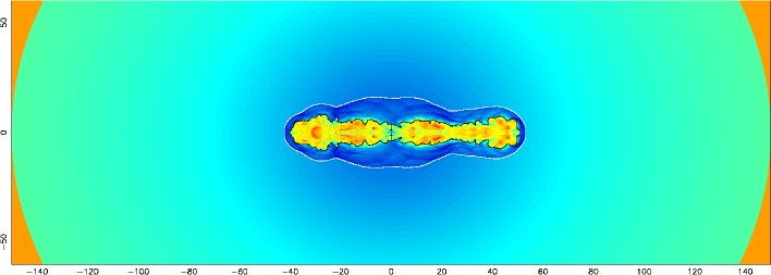
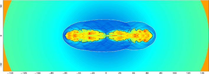
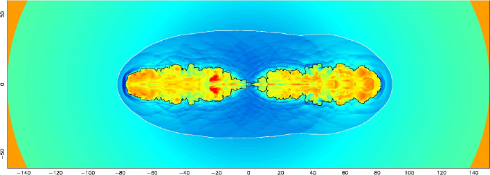
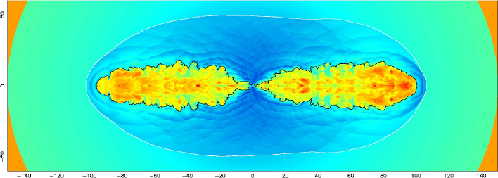
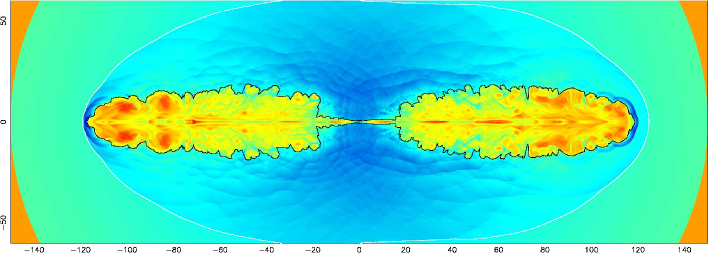
Figure 1: Density in the simulation M25-35-40 for simulation times $t=10$, 20, 30, 40 and 50. The images show a slice through the midplane of the notional 3D volume; as the simulations are axisymmetric, all images are reflection-symmetric about the jet axis. Colours show a logarithmic scale of density between 0.025 and 6.3 simulation units, with dark blue being densest and red least dense. Black and white contours show the lobe and shocked region boundaries respectively, as defined in Section 3. Units of the axes are simulation units ($L_{1}$).

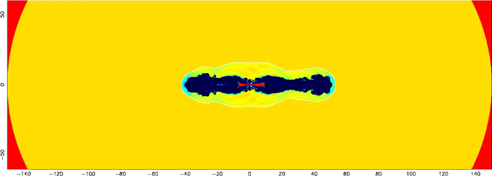
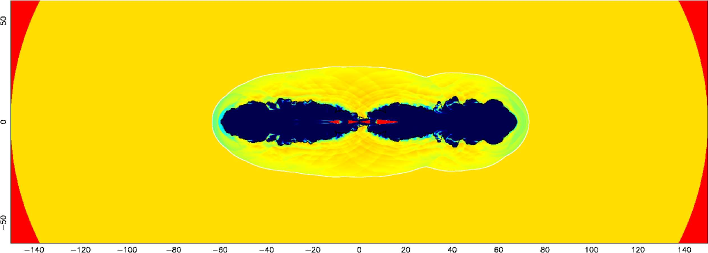
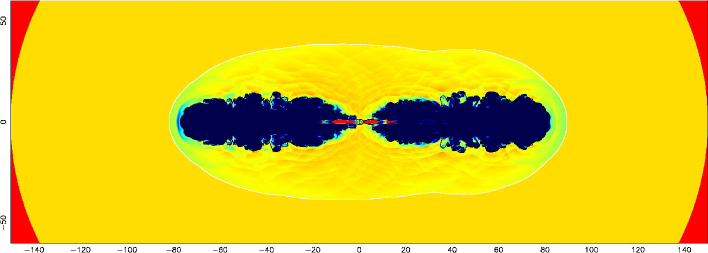
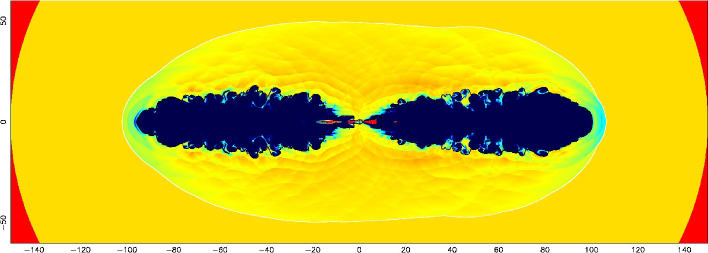
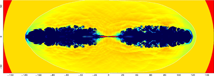
Figure 2: Temperature in the simulation M25-35-40 for simulation times $t=10$, 20, 30, 40 and 50. Notes as for previous figure, but colours show temperatures between 0.32 and 3.2 simulation units, with dark blue being hottest and red coldest.

4.2 Dynamics of the radio lobes

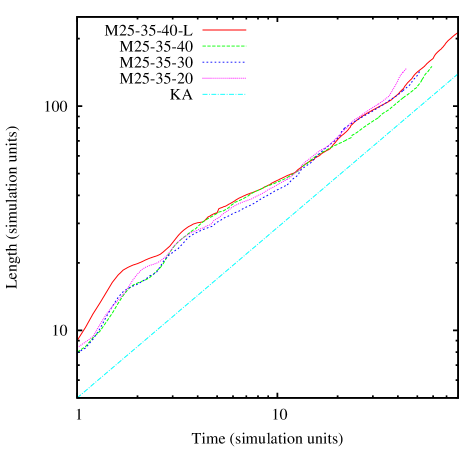
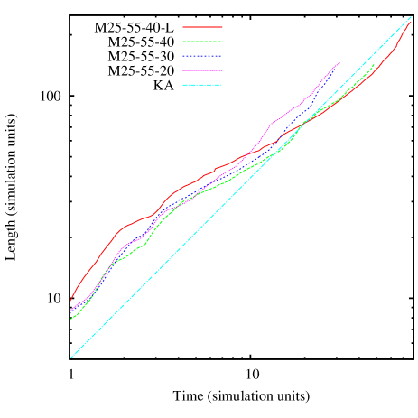
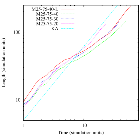
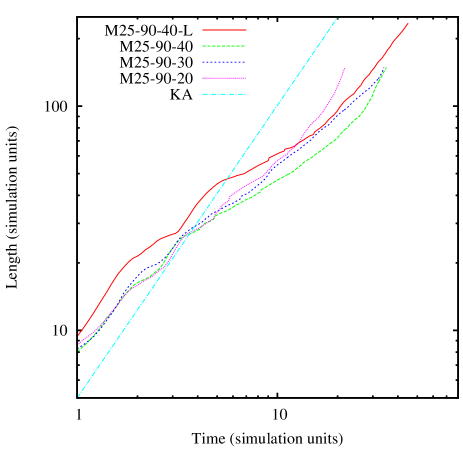
Figure 3: Mean lobe length as a function of simulation time in ${\cal M}=25$ simulations for (top left) $\beta=0.35$, (top right) $\beta=0.55$, (bottom left) $\beta=0.75$ and (bottom right) $\beta=0.90$. Also plotted (‘KA’), with arbitrary normalization, are the Kaiser & Alexander (1997) predictions for a power-law atmosphere.

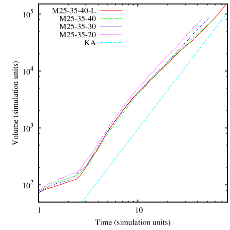
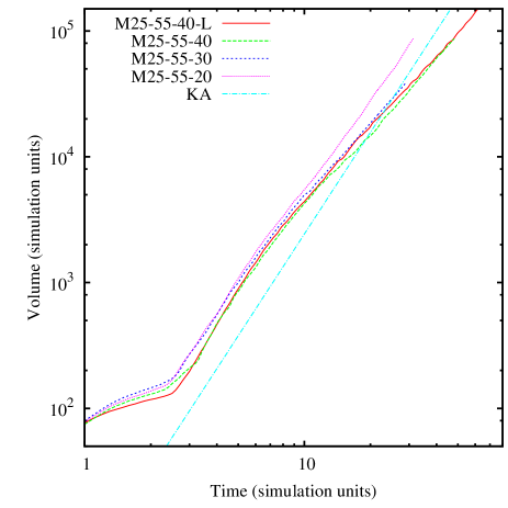
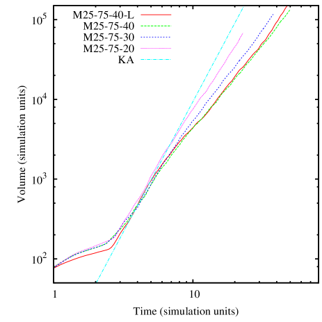
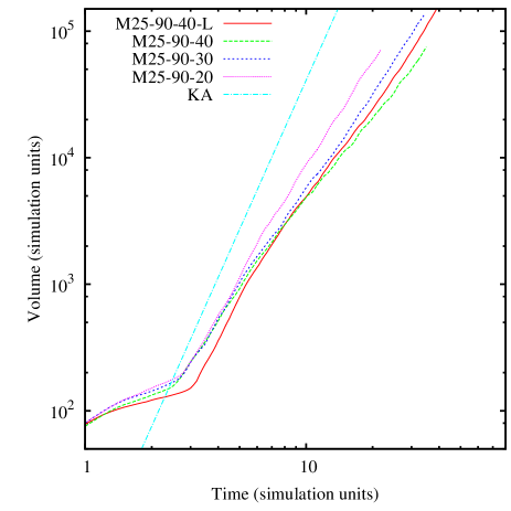
Figure 4: Mean lobe volume as a function of simulation time in ${\cal M}=25$ simulations for (top left) $\beta=0.35$, (top right) $\beta=0.55$, (bottom left) $\beta=0.75$ and (bottom right) $\beta=0.90$. Also plotted (‘KA’), with arbitrary normalization, are the Kaiser & Alexander (1997) predictions for a power-law atmosphere.

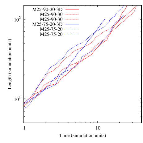
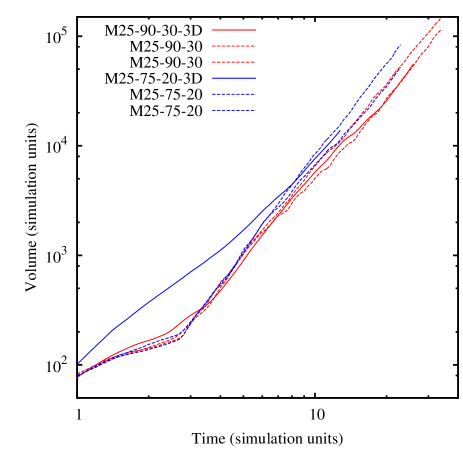
Figure 5: Length and volume as a function of simulation time for the two 3D simulations (solid lines) and the two lobes of the corresponding 2D simulations (dashed lines).

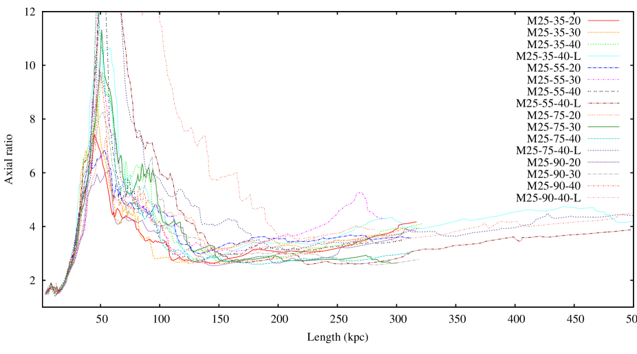
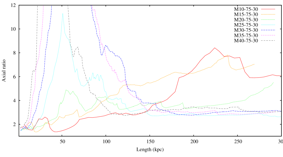
Figure 6: Axial ratio as a function of lobe length in kpc for (top) all the ${\cal M}=25$ simulations and (bottom) simulations with varying Mach numbers but $\beta=0.75$, $r_{\rm c}=62$ kpc.

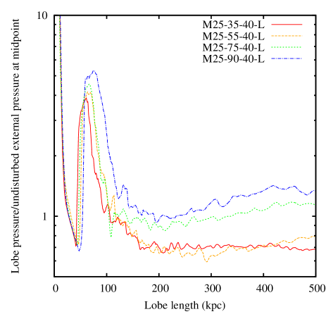
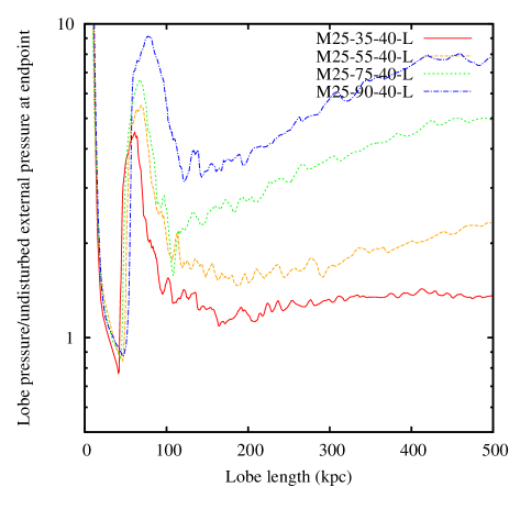
Figure 7: The ratio between mean pressure in the lobes and undisturbed external pressure at (left) the lobe midpoint and (right) the end point of the lobes as a function of lobe length. Only the results from the long simulations are plotted here, but other runs are similar.

In Figs 3 and 4 we plot the mean length and volume of the lobes in the ${\cal M}=25$ runs as a function of simulation time. Here, for each simulation run, we have taken the average length and volume of the two lobes in order to reduce the scatter and highlight the interesting features. Considering the linear growth of the lobes first (Fig. 3) we can generally pick out three distinct slopes in the plots: an initial rapid growth (where the jet grows quickly without forming much in the way of lobes, as we noted above), followed by a phase of slower growth, followed by more rapid expansion again. As the transition between these last two phases happens on scales comparable to $r_{\rm c}$ (and in fact clearly happens earlier for the sources with smaller $r_{\rm c}$; see Fig. 3), it is natural to assume that it is the result of the lobes emerging from the approximately uniform-density material within $r_{\rm c}$ and starting to probe the approximately power-law density regime seen on large scales. Consistent with this, we have plotted the functional form of the length against time, $L_{L}\propto t^{3/(5-3\beta)}$, from the analytic modelling of KA on these plots (with arbitrary normalization) and we see that this is reasonably comparable to the slope at late times – this is particularly clear in the four runs that go out to radii of 250 simulation units. (We note that these four runs seem systematically slightly offset from the equivalent runs with outer radii of 150 units – we attribute this to the slightly lower resolution of the larger runs, which seems to mean that the lobe is slightly longer at all simulation times shown on these plots.) Thus we reproduce not just the qualitatively expected behaviour – higher $\beta$ should mean faster growth at late times – but also do surprisingly well at reproducing the quantitative predictions of KA.

In the volume plots (Fig. 4) we see a very similar three-phase picture: the lobe expands with relatively slow growth of volume at early times (we explore the meaning of this below), then grows rapidly after about $t=2$ in most simulations, and finally expands more slowly and with roughly a power-law dependence on $t$. The power law we see, though, is systematically flatter than the prediction from KA, $V_{L}\propto L_{L}^{3}\propto t^{9/(5-3\beta)}$. KA’s prediction of course comes directly from their assumption of self-similarity in the lobes, so the fact that $V_{L}$ does not appear to scale as $L_{L}^{3}$ points to the fact, already seen in Section 4.1, that these lobes do not grow self-similarly.

The two 3D simulations show very similar lobe dynamics to their corresponding 2D simulations, as shown in Fig. 5. Over most times the growth of length and volume in 3D is indistinguishable from the 2D results. The only noteworthy difference is that the volume seems systematically larger at very early times, particularly in the M25-75-20-3D simulation which has higher spatial resolution. This reinforces the impression that the initial rapid growth of the lobe is not well modelled, since the results depend on the numerical approach taken. However, the 3D and 2D simulations agree very well after this initial phase.

The non-self-similar growth of the lobes is illustrated in another way by Fig. 6 (top panel) which shows the axial ratios as a function of lobe length for all the ${\cal M}=25$ sources in 2D simulations. We define the axial ratio as the ratio of the lobe length to the full lobe width, measured half-way along the lobe length: this is very similar to the definition used by Mullin, Riley, & Hardcastle (2008). With this definition, large numbers imply thin lobes, small numbers correspond to fat ones. Two important features are seen on this plot. Firstly, we note the very strong peak in the axial ratios at small lobe lengths, which corresponds to the phase where the source is growing rapidly in length at close to constant lobe volume. This phase, which is probably not realistic, is generally over by $L_{L}\sim 50L_{1}$ (or $\sim 100$ kpc) as the initial growth of the source slows down and the lobe begins to inflate. More interestingly, at $L_{L}>50L_{1}$ we see a steady growth of the axial ratio as a function of lobe length; that is, throughout most of the lobes’ growth, the lobes are getting thinner as they expand. This is because, while the growth in length of the source is determined by the balance between the lobe pressure and the momentum flux of the jet with the density and pressure at the end of the lobes, the transverse expansion of the lobes is driven by the internal lobe pressure only and the external density and pressure are higher. The change in axial ratio with time or lobe length is not consistent with self-similarity, but it is consistent with what is observed (Mullin et al., 2008). Our simulations do not span the full range of axial ratios observed in real sources, but they do lie in the right region of parameter space, and of course a good deal of scatter is introduced into observed axial ratios by projection effects.

Mach number has some effect on the axial ratio, in the sense that simulations with very low ${\cal M}$ do not form realistic lobes at any stage of the run; their lobe volumes remain low and so their axial ratios are high. This is probably because the material in low Mach-number lobes is never shock-heated to high enough temperatures that the pressure in the lobes (which drives the transverse expansion) becomes comparable to the jet momentum flux. Changing the jet properties, e.g. the opening angle, or including some jet precession would probably allow lobes to form in some circumstances, but in any cases such low jet Mach numbers (for the jet powers we are considering) are not physically very plausible. For ${\cal M}\geq 25$, the late-time axial ratio appears more or less independent of Mach number, and is within the range seen in the various ${\cal M}=25$ simulations (though we note that the early phase of fast lobe growth seems even more extreme for ${\cal M}>25$).

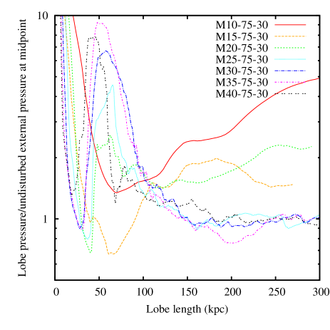
Figure 8: The ratio between mean pressure in the lobes and undisturbed external pressure at the lobe midpoint as a function of lobe length in kpc for varying Mach number.

Finally, we consider pressure balance in the lobes. We compare the mean pressure in the lobes (since the sound speed in the lobes is high, we do not expect any strong pressure gradients internal to the lobes) to the undisturbed external pressure at the midpoints and endpoints of the lobes. This approach is similar to what has been done for radio galaxies, almost exclusively FRIIs, for which the mean lobe pressure can be estimated from observations of inverse-Compton emission and the external pressure from observations of thermal X-ray emission (e.g. Hardcastle et al., 2002a; Croston et al., 2004; Konar et al., 2009; Shelton et al., 2011). Observers use the undisturbed external pressure because this can easily be estimated observationally, e.g. by masking out the lobes and fitting spherically symmetric projected $\beta$ models, although of course the lobes are not expected to be in direct contact with this material. What we find is quite striking (Fig. 7): after the initial expansion, and at $L_{L}\approx L_{2}$ the lobes come into, and remain in, rough pressure balance (within better than a factor 2) with the external pressure at the lobe midpoint, though they are consistently strongly overpressured with respect to the external pressure at the ends of the lobes (as expected since they are seen to drive strong shocks at all times: Section 4.1). Thus the simulations reproduce a key observational result. We also see (Fig. 8) that this result is independent of Mach number so long as the Mach number is high enough that realistic lobes form (${\cal M}\geq 25$). The 3D simulations reproduce these 2D results.

Overall, the simulations seem to do reasonably well at late times at reproducing the behaviour we expect from real radio galaxies. At early times, they are not realistic, as noted above. Only when the lobe has grown to a size comparable to the core radius do we enter a regime that is comparable to the behaviour of real radio galaxies. However, once the simulations enter that regime, they seem to stay there, independent of jet Mach number, so long as it is high enough, and of the dimensionality of the simulation. This means that it is reasonable to consider the energetic effects of the radio source in its environment, as long as we confine ourselves to the period after $t\sim 5$ or so when the lobes are fully established.

4.3 Energetics of the lobe/environment interaction

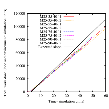
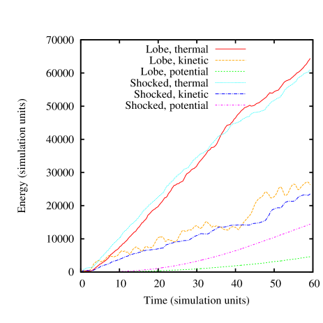
Figure 9: Left panel: the total energy stored in the jets, lobes and external environment as a function of simulation time for each lobe of the four ${\cal M}=25$ simulations with $r_{\rm c}=40$, together with the expected slope as discussed in the text. Right panel: the energy budget of the lobes and shocked region in the simulation M25-35-40 as a function of simulation time.

In this subsection we consider the energetics and environmental impact of the lobes.

The first and most basic test is to check whether the jets are carrying the expected level of energy into the simulation as a function of time. The simulation energy unit $\epsilon$ is $\rho_{0}L_{1}^{3}c_{s}^{2}$, or around $4.6\times 10^{49}$ J for our reference simulations with ${\cal M}=25$. So we can easily compare the rate of growth of energy in the lobes and environment with the expected jet power $Q_{0}$, or, equivalently, we can calculate the expected input power in simulation units (${\cal M}^{3}/8$) to see whether the simulations are conserving energy as expected. The results of such a comparison are shown for some representative simulations in Fig. 9. There are several points to note from this figure. Firstly, we see that there is a short period at the start of every simulation plotted where the total energy in the simulations stays constant, rather than increasing. In detail, it seems that the jet stops flowing into the simulation volume at these times: because the jet is implemented as a boundary condition, it is possible for the jet’s entry on to the grid to be blocked, e.g. by backflow, with no energetic consequences. Once the jet is established, though, we see an approximately linear growth of energy with time, though note the superposed oscillation which is a result of the slight sinusoidal variation imposed on the Mach number (Section 2); we plot the two lobes separately in this figure so that the different phases can be seen. Finally, we note that although the gradients in different simulations are in close agreement, they disagree with the expected slope at around the 10 per cent level, even after a non-zero start time is imposed to account for the fact that a persistent jet only starts at around $t=3$. As we see slightly different slopes for our runs with slightly different resolutions, we believe this discrepancy to be the result of resolution effects connected with the implementation of the jet as a boundary condition. In particular, it seems that the very edges of the jet have a lower density than they should have even at the inner radius, so that less energy enters the simulation than our simple calculation suggests. However, such structures at the jet inlet should stay constant with time, and this is consistent with the fact that the missing power is also constant with time. If there were significant errors in conservation of energy in the simulations, or in the calculations done in post-processing, we would expect the curves in plots like those of Fig. 9 to be non-linear with time, given that the growth of the lobes and the shocked regions is very clearly non-linear. As this is not the case, we are confident that the simulations can be used to study the energetic impact of the expanding lobes after early times; as noted above, the dynamics of the lobe are not realistic at early times anyway.

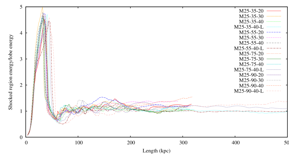
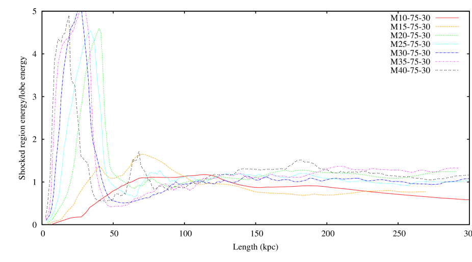
Figure 10: The ratio between the energy stored in the shocked region and the lobes as a function of lobe length; top, for all ${\cal M}=25$ simulations; bottom, for simulations with different Mach number and $\beta=0.75$, $r_{\rm c}$ = 62 kpc.

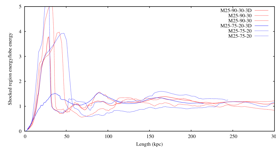
Figure 11: As for the top panel of Fig. 10, but the two 3D simulations are shown compared to the results for individual lobes of the comparator 2D simulations. Solid lines show the 3D simulations and dashed lines the 2D ones. No significant differences between the 2D and 3D results are seen after $L\sim 50$ kpc.

Our post-processing accounts separately for the thermal, kinetic and potential energies in both lobes and in the corresponding shocked regions. Thus we can investigate how the work done by the jet is distributed between these different contributions to the total energy. An example of this type of analysis is shown in Fig. 9. We see that, as might be expected, the thermal energy in the lobes and the shocked region dominates over the other components. Kinetic energy is non-negligible in both, however, accounting for something like a third of the total. At late times the potential energy of the shocked material, i.e. the work done in lifting shocked material out of the centre of the galaxy, also becomes important. There are strong variations in the kinetic energy of the lobe material, which partly reflect the imposed variations in Mach number of the injected jet, but also show the effects of the repeated internal shocks in the lobes.

Perhaps the most obvious feature of this plot is that the thermal and kinetic energy stored in the lobes keeps remarkably well in step with that in the shocked region over most of the lifetime of the source. We can quantify this for the simulated sources in general by plotting the ratio of the total energy stored in the shocked region to that in the lobes (Fig. 10). We see that at all lengths (times) after the regular lobe growth is established ($L=30L_{1}$, corresponding to $t\sim 3$), the ratio of external to internal energies is close to unity, with no very strong dependence on the parameters of the environment (there does seem to be a weak dependence, in the sense that this ratio tends to be higher for higher $\beta$ values). This result confirms earlier findings in MHD simulations by O’Neill et al. (2005) and Gaibler et al. (2009), but is based on a much more comprehensive sampling of parameter space. We return to this very important result in Section 5.

Like others we have considered above, this result appears more or less independent of Mach number within the range we have used (Fig. 10): even in the low-Mach-number systems where realistic lobes are not formed, the energy ratio does not differ strongly from unity at late times. It is also reproduced in the 3D simulations (Fig.11).

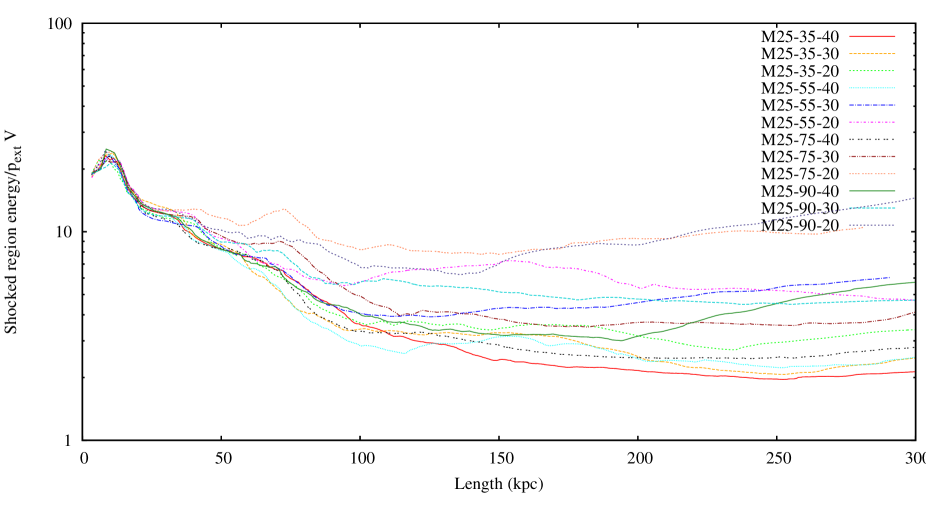
Figure 12: The ratio between the energy stored in the shocked region and $p_{\rm ext}V$ as a function of lobe length for the standard-sized ${\cal M}=25$ simulations.

Finally, we can compare the work done on the external medium with commonly used methods for estimating it. As we have seen, the internal energy in the lobes tracks that in the shocked region reasonably well over most of the lifetime of the source (Fig. 9). Therefore, if the internal energy of the lobe can be estimated, the work done on the external medium can be estimated too. Many literature estimates of the work done (e.g. Bîrzan et al., 2004) assume that it is $\sim pV$, where $p$ is some relevant pressure and $V$ is the volume of the lobe, or of the observed X-ray cavity. This must be of the right order of magnitude, but setting aside the problems in estimating $V$ in real radio galaxies, where projection effects are important, the question is what value of $p$ to adopt. If the internal pressure of the lobe (e.g. from inverse-Compton emission) is known, then this is easy, but in this case of course we know the internal energy density of the lobe as well. If the internal pressure is not known, then our results above suggest that the undisturbed external pressure at the lobe midpoint can give a reasonably good estimate of it. In this case, we can use our simulations to see how badly in error a simple $p_{\rm ext}V$ estimate is.

The ratio between the work done on the external medium and $p_{\rm ext}V$ is plotted in Fig. 12. If the radio source were in pressure balance with the external medium at the midpoint, and if all the energy in the lobe were thermal energy, then we would expect this ratio to have a constant value of 1.5 for roughly equal internal and external energy. However, the fact that some of the work done on the lobes is in the form of bulk k.e. and that the midpoint pressure balance is only approximate causes deviations from this relationship; factors in the range 2–10 are typical. In detail, the trends in Fig. 12 are readily understood. At early times, all simulated radio sources are strongly overpressured and drive strong shocks. Consequently, the ratio is high; it decreases as the source comes close to pressure balance. The simulations with smaller core radii and larger $\beta$ show higher ratios presumably because they are further from pressure balance over most of their length; therefore, at late times, for our smaller core radii and larger values of $\beta$ we generally find values closer to 10, whereas for large core radii and small betas the ratio tends towards two. To summarize, although the exact numerical factor is likely to be different for real radio galaxies, with a relativistic adiabatic index, it is safe to say that $p_{\rm ext}V$ pressure estimates are likely to underestimate the work done on the external medium by a factor of a few; moreover, this factor will depend on the age of the radio galaxy and the environment in which it resides. Of course, it should be noted that our results apply principally to FRII radio galaxies, while many of the objects showing cavities are lower-power FRIs; although qualitatively we might expect similar caveats to apply to a $p_{\rm ext}V$ analysis of FRIs, our simulations do not allow us to make quantitative statements about such systems.

4.4 Radio emission

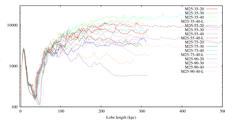
Figure 13: Radio luminosity (simulation units) as a function of mean lobe length for the ${\cal M}=25$ simulations.

Our simulations do not contain all the physics needed (i.e., electron acceleration, loss processes and magnetic fields) to carry out a proper visualization of the synchrotron emission from the lobes. It is, however, interesting to ask how the overall radio luminosity of the lobes would evolve with time, and we can do this by assuming that the pressure that we measure in the lobes is contributed by electrons and magnetic field. Since the simulations do not constrain the contributions of these separately, we need to assume equipartition or some constant departure from equipartition (as measured by inverse-Compton observations, e.g. Croston et al. 2005). Let the energy density in electrons be $U_{e}$ and that in magnetic field be $U_{B}$, then this assumption corresponds to

$$\eta U_{e}=U_{B}=\frac{B^{2}}{2\mu_{0}}$$

where $\eta$ describes the energetic departure from equipartition, $\eta<1$.

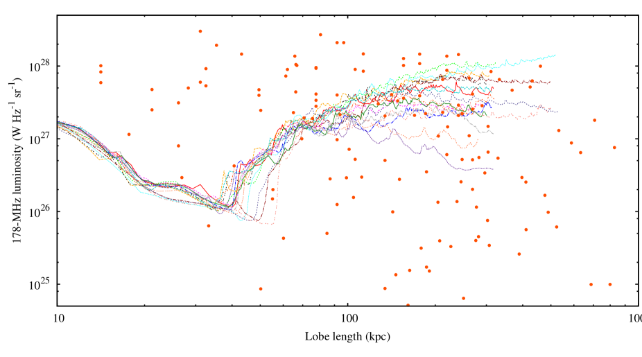
Figure 14: Radio luminosity (physical units) as a function of mean lobe length for the ${\cal M}=25$ simulations, converted from simulation units using the factor ${\cal L}$ for $\eta=0.1$ as described in the text. The line styles correspond to the same simulations as in Fig. 13. Overplotted are the 3CRR radio galaxies above the nominal FRI/FRII cutoff of $5\times 10^{24}$ W Hz^-1 sr^-1, where we have scaled down the largest angular size by a factor $\sqrt{2}$ to account for the fact that the simulations are for a single mean lobe length and that a typical 3CRR source will be projected. Note that the different curves represent radio sources with the same jet power, but in different environments. The radio luminosity increases in environments with a larger core radius and shallower density decline.

If we then assume a power-law electron distribution, it can be shown using standard textbook results (e.g. Longair, 2010) that the volume emissivity goes as $p^{(q+5)/4}$, where $q$ is the electron energy power-law index; the luminosity can be calculated by integrating this over the lobe volume. Taking $q=2.2$, corresponding to a low-frequency spectral index $\alpha=0.6$, the emissivity scales as $p^{1.8}$. We begin therefore by plotting $\int p^{1.8}{\rm d}V$ over the simulation volume as a function of lobe length (Fig. 13). These plots correspond to the ‘tracks in the $P$–$D$ diagram’ commonly used in studies of the evolution of radio galaxies, albeit still in simulation units at this point. We see first of all that the ‘luminosity’ in these plots varies strongly with source length (and therefore time). Ignoring the strong variation before the lobe is properly established at $L<50$ kpc, we see a general trend for the luminosities first to scale up and then to level out. At the longest lengths, the luminosities may level out or decrease slightly, the most obvious decreases being seen in environments with high $\beta$ and small $r_{\rm c}$. At $L\sim 200$ kpc, there is almost an order of magnitude difference in the radio luminosities of sources with, by construction, identical jet powers. We also note the smaller-scale, random or slightly periodic variations in the radio power; these reflect fluctuations in the pressure in the lobes and should not be taken too seriously, since the detailed hydrodynamics in the lobes is probably not correct.

It is important to note that the analysis described here takes no account of radiative losses. The approximation that the electron energy distribution is a power law is not a bad one even when radiative losses are effective, because the energy density in the electrons is dominated by low-energy electrons with long loss timescales; but of course the frequency $\nu$ needs to be low in order to sample the part of the synchrotron spectrum that is still adequately represented by a power law. Since we wish to compare these radio luminosities to real luminosities, we use a notional observing frequency of 178 MHz, which should be low enough to avoid significant spectral ageing effects in all but the oldest sources, and allows direct comparison to observations of the 3CRR sample and to the work of Kaiser, Dennett-Thorpe, & Alexander (1997).

Given that the simulation unit of pressure is $P=\gamma n_{0}kT$, or $1.6\times 10^{-11}$ Pa, and the unit of volume is $L_{1}^{3}$, it can be shown that the simulation unit of radio luminosity in physical units (W Hz^-1 sr^-1) is

$${\cal L}=c(q){\frac{e^{3}}{\epsilon_{0}cm_{e}}}\left({\frac{\nu m_{e}^{3}c^{4}}{e}}\right)^{-\frac{q-1}{2}}\frac{3P^{\frac{q+5}{4}}}{4\pi I}(6\mu_{0}\eta)^{\frac{q+1}{4}}(1+\eta)^{-\frac{q+5}{4}}L_{1}^{3}$$

where $e$ is the charge on the electron, $m_{e}$ its mass, $c$ the speed of light, $\epsilon_{0}$ the permittivity of free space, $\mu_{0}$ the permeability of free space, $I$ the integral of $EN(E)$ over the energy range of the electrons, $E_{\rm min}$ to $E_{\rm max}$, and $c(q)$ a dimensionless constant, the product of a number of gamma functions, of order 0.05. Taking $q=2.2$, $\nu=178$ MHz, $\eta=0.1$ (given that the measured magnetic field strengths can be up to a factor of a few below equipartition, see Croston et al. (2005), $E_{\rm min}=10m_{e}c^{2}$, and $E_{\rm max}=10^{5}m_{e}c^{2}$ (the results are insensitive to this choice of electron energy range), we find that ${\cal L}=6.6\times 10^{23}$ W Hz^-1 sr^-1 for the ${\cal M}=25$ simulations. If we take $\eta=1$, the conversion factor roughly doubles, ${\cal L}=1.4\times 10^{24}$ W Hz^-1 sr^-1, so that we are not excessively sensitive to equipartition assumptions.

This conversion factor allows us to generate a plot of the evolution of radio luminosity in physical units for the ${\cal M}=25$ sources (results for other Mach numbers are similar but are omitted for clarity). We overplot data for the 3CRR sources (Fig. 14; note the change of $x$-axis scale from linear to logarithmic). We see immediately that the luminosities are in the right general area of parameter space for powerful radio galaxies; of course, the 3CRR FRIIs we have overplotted should represent a wide range of jet powers and environments, down to objects with $Q\sim 10^{36}$ W in very poor groups (e.g. Hardcastle et al., 2012), so it is not surprising that the simulations do not sample the full $P-D$ diagram. Within the limitations of the simulations and the calculation we have carried out (i.e., a comparison is only possible for $L>50$ kpc, and we neglect losses, which may well be significant on scales $>300$ kpc) we view the position of our simulation tracks on this plot as good evidence that we are generating physically reasonable radio sources. We note that the typical luminosity, $\sim 10^{27.5}$ W Hz^-1 sr^-1, is exactly what we would expect from a $10^{38}$ W jet using the results of Willott et al. (1999), which, if a coincidence, is certainly a remarkable one.

Having said this, it is striking that the most luminous sources in the simulations (those located in large-$r_{\rm c}$, low-$\beta$ environments) approach the highest luminosities seen for 3CRR sources, which is perhaps surprising given that we are only trying to simulate intermediate-power FRIIs with $Q=10^{38}$ W; however, these environments are very rich, perhaps unrealistically rich for most low-power 3CRR sources, and so we do not regard this as a significant problem. We also note that any non-radiating particle content in the lobe (see Hardcastle & Croston 2010 for a discussion of the evidence for these in FRIIs) would tend to reduce the required electron number densities and hence the radio luminosity.

Finally, it should be noted that the very strong dependence of luminosity on environmental properties on 100-kpc scales, which is independent of these caveats, provides both a quantitative estimate of the boosting effect of rich environments discussed by Barthel & Arnaud (1996) and a useful warning of the dangers of attempting to infer jet power from radio observations alone. On these scales, there is at least an order of magnitude scatter in the radio luminosity expected for a fixed jet power. We return to this point in Section 5.

4.5 X-ray emission

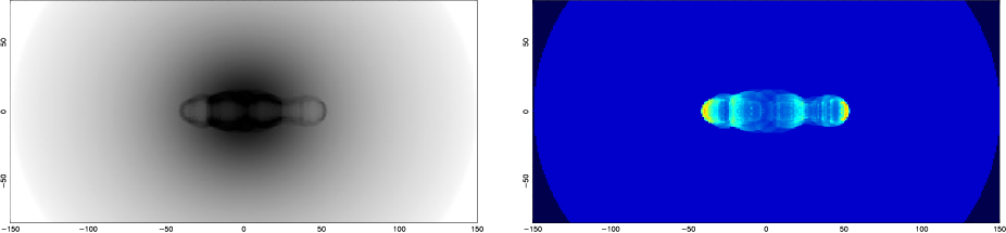
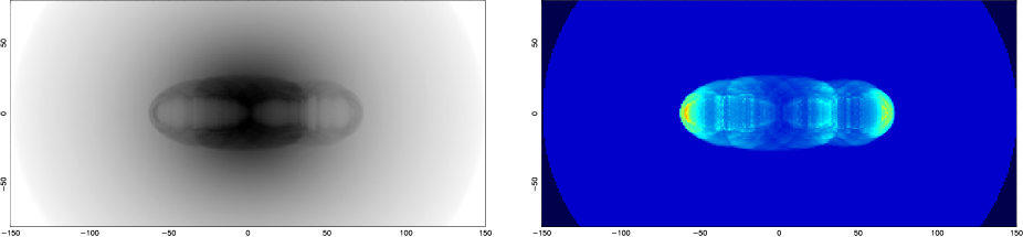
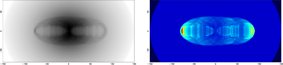
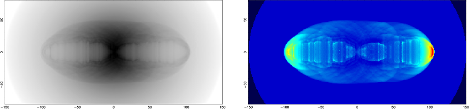
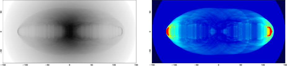
Figure 15: X-ray visualization of the simulation M25-35-40 for simulation times (from top to bottom) $t=10$, 20, 30, 40 and 50. The left-hand images show Chandra counts in the energy range 0.5–5.0 keV, with a linear transfer function. The right-hand images show the corresponding emission-weighted temperature, with dark blue being coldest (1.8 keV) and red being hottest ($>3$ keV); see the text for discussion. The jet axis is at 90^∘ to the line of sight and the image resolution is 1 simulation unit ($\sim 2$ kpc). Compare Figs 1 and 2, which show slices through the midplane of this simulation at high resolution. Co-ordinates shown are simulation units.

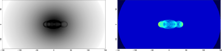
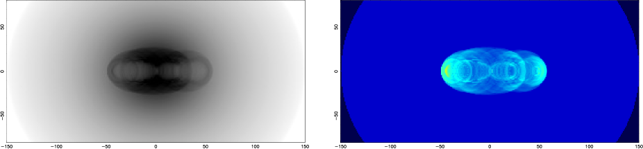
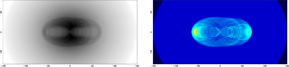
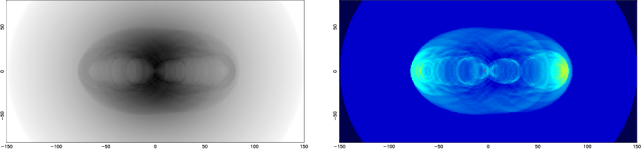
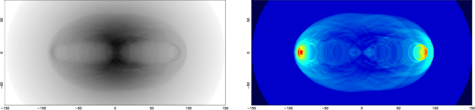
Figure 16: As for Fig. 15, but the jet axis is at 45^∘ to the line of sight.

We can assess the observable effect of the radio galaxy’s interaction with its environment in these models by visualizing the X-ray emission from the environment. We choose to model X-ray emission as seen by Chandra: Chandra’s angular resolution of $\sim 0.5$ arcsec gives a spatial resolution of $\sim 2$ kpc at around $z=0.2$, so we adopt a spatial resolution of 1 simulation unit for the ${\cal M}=25$ simulations. We assume that lobe material does not contribute to the X-ray emission, and therefore exclude it using the tracer. We use xspec with a real Chandra response file to model the conversion between emission measure and (on-axis) count rate in the 0.5–5.0 keV energy band as a function of temperature for an APEC model with 0.3 solar abundance (neglecting Galactic absorption). We can then compute the expected X-ray image (for infinite signal-to-noise) by integrating along lines of sight through the simulated volume: we neglect emission outside the simulation (corresponding to perfect background subtraction). We can also compute the emission-weighted (strictly, counts-weighted) mean temperature along the line of sight; Chandra does not quite measure this quantity, but it is close enough to give an idea of the expected observational effects. We show representations of the counts image and the map of emission-weighted temperature for several times during the simulation M25-35-40 and for two different angles to the line of sight in Figs. 15 and 16.

Bearing in mind that we are ‘observing’ with infinite signal to noise and that therefore many of the details seen in the simulations are not likely to be visible in reality, these visualizations are qualitatively very consistent with real observations. We note first of all that, though there is an approximately elliptical shock with a clear surface brightness contrast at the boundary, the measured temperature difference across the shock is not likely to be very great; the emission-weighted temperature of the shocked region is $\sim 2.5$ keV compared to the unshocked 2-keV gas. This compares very well to the modest temperature increases seen in this region in Cygnus A (Wilson et al., 2006). The regions of strong shocks and high temperatures ($>3$ keV) are confined to the very tips of the lobes, and even then are not always present; it is easy to imagine that these high temperatures will be hard to observe in real radio galaxies, where measurements of spectra require integration over large regions. One is more likely to see moderately increased temperatures over a larger region at the head of the lobes, as suggested in the case of Cygnus A by Belsole & Fabian (2007) and in 3C 452 by Shelton et al. (2011). Cavities are visible, but again quite low in surface brightness contrast, and so not necessarily expected in real observations (particularly as we have not attempted to model inverse-Compton emission from the lobes, which in real observations will fill in some of the cavity emission). The most obvious feature of the simulated observations, which should be present in any real observation if these simulations are well matched to reality, is the emergence of a bright central ‘bar’ of X-ray emission, together with ‘arms’ extending along the inner part of the lobes. This material is cool, with a temperature equal to, or even in places slightly less than, the original temperature; it is generated from the pre-existing dense core of the host cluster, which is initially heated by the radio-lobe shock but then cools adiabatically as the shocked region expands ahead of it, in the manner discussed by Alexander (2002). (Radiative cooling of the thermal material might be expected to enhance the density contrast here still further.) Structures like this, positioned roughly inside the boundary of the radio lobes (though note that projection will affect the lobes and the bar/arms structure differently, so that we do not expect an exact match between the two) are a smoking gun for a system in which the lobes have come into pressure balance at large radii and are now being squeezed out as in Model C of Scheuer (1974). In real observations, structures that could be interpreted in this way are in fact ubiquitous in observations of FRIIs; examples include the central, bright, cool structure in Cygnus A (Wilson et al., 2006), the very obvious bar and arms in 3C 444 (Croston et al., 2011), the ‘ridges’ in 3C 285 and 3C 442A (Hardcastle et al., 2007) and in 3C 401 (Reynolds et al., 2005). In the best-studied cases with the clearest evidence for ongoing strong shocks (Cygnus A and 3C 444) the ‘bar’ and ‘arm’ temperatures are consistent with the unshocked cluster temperature, precisely as expected in our models. The agreement between our simulations and the observations of 3C 444, which is an FRII at $z=0.153$ with a slightly higher jet power embedded in a slightly richer environment, is very striking; forthcoming deep XMM-Newton observations of this object may provide the opportunity for a detailed test of the model’s temperature predictions. This should be combined with sensitive low-frequency observations, e.g. with LOFAR, to establish exactly how the lobes relate to the X-ray structures.

4.6 Suppression of cooling?

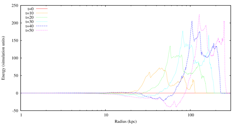
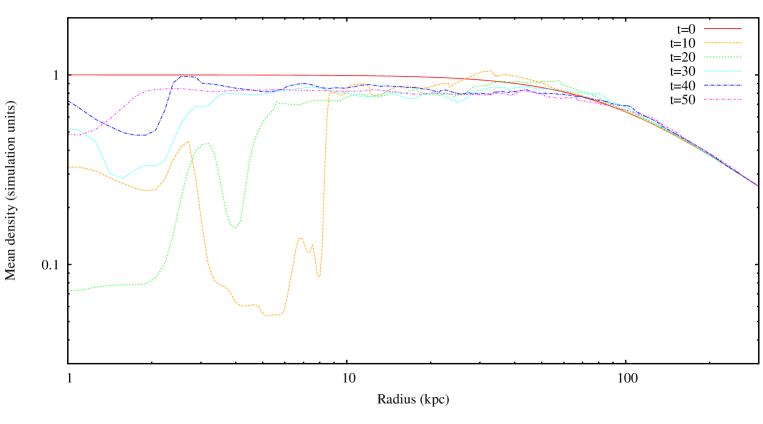
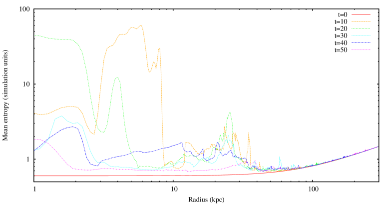
Figure 17: Radial profiles of excess energy, number density and entropy in the external medium as a function of radius for 6 different times in the M25-35-40 simulation. The excess energy profile (note linear scale on the $y$ axis) shows total energy (thermal and kinetic) in all the cells that are not inside the lobe at a given radius, minus the value in those cells at $t=0$. The density and entropy profiles are the volume-weighted mean values at each radius. See Figs 1 and 2 for images of the simulated density and temperature in this simulation at these times ($t>0$).

Our simulation setup was explicitly designed so that the jet power of the FRII exceeds by roughly an order of magnitude the bolometric X-ray luminosity of the simulated cluster environment. But this is not a sufficient (nor indeed a necessary) condition for suppressing radiative cooling of the X-ray-emitting material, because the cooling rate is a strong function of density and thus of radius, and the key requirement for prevention of the traditional cooling catastrophe is to suppress cooling at the centre of the group/cluster. While numerical modelling shows that powerful, FRII-like radio galaxies can suppress cooling (e.g. Basson & Alexander, 2003), it has been clear for some time (e.g. Omma & Binney, 2004) that they are not an efficient way of doing so, because the bulk of the energy/entropy injection takes place on scales that are much larger than the cooling radius (i.e. the radius within which the cooling time is less than some threshold value). In sources like ours, which are intended to come into pressure balance at the centre at late times, the situation is even worse, because there is little or no energy input at the centre of the cluster at all, while the increase in axial ratio with length also means that less of the available volume of the cluster is affected at late times. However, the cluster cores do undergo significant heating early in the simulations.

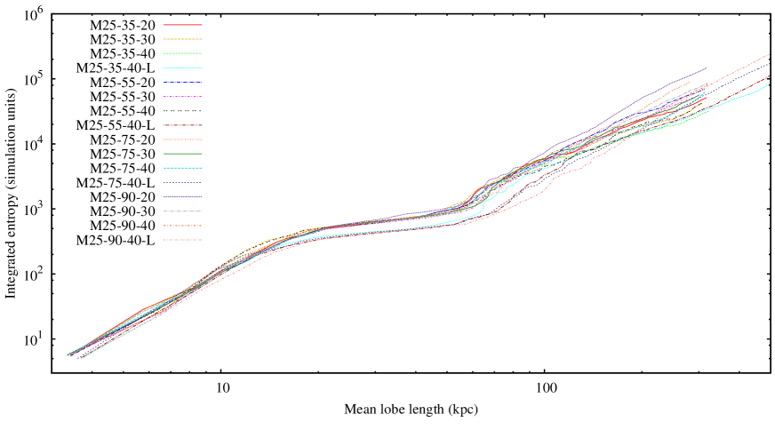
Figure 18: Integrated excess entropy as a function of lobe length for the simulations with ${\cal M}=25$. A baseline corresponding to the initial ($t=0$) entropy of the gas inside the shock front has been subtracted from all values plotted. The slope of this plot gives a measure of the efficiency with which the radio galaxy irreversibly heats the external medium as it grows. The three distinct regions here can be understood in terms of the three phases of lobe growth speed, and therefore shock speed (Fig. 3); weaker shocks have a lesser effect on entropy (Kaiser & Binney, 2003).

We can quantify these effects in our simulations by looking at radial profiles of some quantities related to cooling as a function of simulation time. Fig. 17 shows an example provided by the M25-35-40 run, but all our results are broadly similar. What we see is that, as expected, the total energy input to the atmosphere is mostly co-located with the front of the lobes. The energy input to the atmosphere at small radii is actually negative, because the effect of the radio galaxy is to remove gas from the central regions without providing much in the way of long-term heating in these locations. This can be seen in the density profiles in Fig. 17 – in the short term, the radio source has a dramatic impact on the density of hot gas in the central regions, but as the central pressure drops and material flows in behind the radio lobes the mean density profile rapidly recovers to something not very dis-similar to its original shape behind the shock front. Similarly, the entropy profiles – here we are plotting the entropy index, $\sigma=Pn^{-5/3}$ (Kaiser & Binney, 2003) in simulation units – show a very marked effect at early times but only a very modest increase in the entropy in the central regions of the plot at late times. The effect on cooling time (proportional to $T^{1/2}/n$: not plotted) is very similar to that on entropy. Note also the almost completely negligible effect of the radio source on the entropy profile at large radii – this is because these are volume-averaged radial profiles, and at these large radii very little of the volume of the cluster is actually affected by the radio galaxy.

Why do we see this behaviour of the entropy index? In our simulations, entropy is generated at shock fronts, redistributed in mixing regions, and conserved otherwise. The strong entropy increase in the whole core region at early times means that this gas must in the end rise – either buoyantly or by being carried out by the expanding radio source – out of the centre of the cluster; in other words, much of the core has been efficiently heated. However, the core is then refilled by adjacent gas from larger initial radii. Correspondingly, the density decreases in this region. Therefore, while the effect of the jet was to increase the entropy of much of the gas that was in the core initially by a factor of several tens, the gas that is in the core at the end of the simulation has only a 10-20 per cent higher entropy than the initial conditions in this region. Because the radio galaxies continue to drive strong shocks at large radii, they continue to increase the entropy of the shocked gas at all times: this can be seen in a plot of the integrated entropy, $\int\sigma{\rm d}N$, as a function of lobe length (Fig. 18). However, as the profiles show, this entropy increase is no longer relevant to the cooling core, or significant over the total volume of the cluster.

We conclude that long-lived FRII radio sources with realistic dynamics are not expected to be very efficient at suppressing cooling in this type of environment. Though much of the energy is thermalised and ends up in the ambient gas, only the central parts of the cluster are efficiently, irreversibly heated, and much of this material then leaves the central regions; at late times (i.e. $\sim 10^{8}$ years after the radio activity begins), there are only very modest effects on the central entropy and cooling time. To couple AGN output effectively to the gas with short cooling times in the centres of clusters, radio sources need not to grow beyond the central cluster scale, so that they are continually in the early-time regime seen in Fig. 17. An excellent way of doing this is to make the radio source intermittent (see e.g. Mendygral et al., 2012) and observations of the centres of cool-core clusters such as Perseus show that this is what happens in nature most – but not all! – of the time. One of the key questions to be solved in ‘AGN feedback’ models must be how the AGN in cool cores ‘know’ that they are required to be intermittent in this way while other radio galaxies, like the classical doubles, can exhibit long-term persistent jet activity.

5 Summary and conclusions

We have carried out high-resolution, 2D axisymmetric hydrodynamical simulations of the evolution of the lobes of radio galaxies in a wide range of realistic environments. The simulations are intended to be closely matched to the physical conditions known to obtain in the environments of FRII radio galaxies, and to probe all size scales from the collimation of an initially conical jet up to (and beyond) the size scale at which the lobe pressure is expected to drop below the pressure in the external medium. Although the details of the dynamics internal to the lobe are probably not realistic, we argue that the energetics of the interaction with the external medium should be unaffected by this so long as there is a mechanism that efficiently ‘thermalizes’ the kinetic energy supplied by the jet, as is the case in our simulations once the lobes grow to a few tens of simulation lengths in size.

The key results of our work appear to be independent of both environment and initial jet Mach number, within the range that we have been able to probe, and can be summarized as follows:

1. As expected both from observations and from the design of our simulations, the lobes do come into pressure balance with the external medium in the course of the simulations (Section 4.1, Section 4.2). At late times, the lobes are driven away from the centre of the host cluster by dense, high-pressure ICM. Thus the lobe growth is more consistent with Model C than with Model A of Scheuer (1974), or, equivalently, we observe the ‘cocoon crushing’ process of Williams (1991). Lobe growth is not self-similar, and indeed axial ratios tend to increase with time on hundred-kpc scales, consistent with what is observed (Section 4.2).

2. Unsurprisingly, given the above, the models of KA do not describe some of the behaviour of the simulated radio galaxies (Section 4.2). The late-time length of the sources as a function of time is not badly described by the relations derived by KA, which is not surprising since the environment has close to a power-law behaviour of density with distance on these scales and the momentum flux of the jet, distributed over the ‘working surface’, continues to drive the linear expansion of the radio source. However, the KA relations significantly overestimate the growth of lobe volume with time.

3. The pressure of the undisturbed external environment at the midpoint of the lobes is a reasonable, though not perfect, estimator of the pressure in the lobes once normal lobe growth is established (Section 4.2). Lobes remain strongly overpressured with respect to the ambient medium at their tips. This reproduces a key observational result based on estimates of the lobe pressure from inverse-Compton observations.

4. The work done by the radio galaxy on the environment (including the thermal, kinetic and potential energy of the shocked gas) is very close to the internal energy (thermal and kinetic) of the lobes at all times once the lobes are established (Section 4.3). A simple $p_{\rm ext}V$ estimate of the work done by the lobes underestimates it by a factor of a few (up to an order of magnitude in extreme cases).

5. The simulated radio galaxies can reproduce the approximate radio luminosities of real 3C radio sources whose jet powers are believed to be comparable (Section 4.4). However, there is a large scatter (well over an order of magnitude) in the radio powers expected from sources of the same power (as all our simulated sources are) in different environments.

6. X-ray visualization of our simulations (Section 4.5) makes some predictions for the morphological and temperature structure that we should observe that are in principle testable, and that show striking similarities to what is observed in a few well-studied FRII sources.

7. Finally, we note that, as has been known for a while, FRII radio galaxies with realistic dynamics do not couple effectively to the hot medium at the centres of clusters, and therefore are not in general effective at suppressing cooling (Section 4.6), though their energetic impact can be very considerable in localized regions around the lobes in the outer parts of the cluster.

Several of these points have importance for observational work and for models of the energetic impact of radio galaxies on their environments. Firstly, our conclusion that the internal and external energy of the radio galaxy remain in rough balance, independent of the properties of the external environment or the initial jet Mach number, means that there is a very easy recipe for estimating the work done by an FRII radio galaxy on its environment; simply estimate the energy stored in the lobes, ideally using an inverse-Compton observation to measure the lobe magnetic field strength, and one also has, to within better than a factor 2, the work done on the external environment. Although it might be objected that our modelling does not include important features of the physics of radio galaxies, such as magnetic fields, which might be expected to change this conclusion, we are reassured by the similar conclusions reached for specific simulations with more realistic physics, including magnetic fields, by O’Neill et al. (2005) and Gaibler et al. (2009).

Secondly, if we accept that all FRII radio galaxies follow the basic pattern seen in our modelling and come into rough pressure balance with their environments, independent of the initial power of their jets, at around the lobe midpoint, once they have grown to a sufficiently large scale (i.e. once they are in a roughly power-law atmosphere?), then this means that large-scale FRIIs provide a probe of the pressure of their environments; if one observes an FRII on hundred-kpc scales, the external pressure at its midpoint should be of order the internal pressure, which can again be assessed by inverse-Compton observations or, with some assumptions about magnetic field strength, from synchrotron emission alone. In the coming decades, where deep radio observations may be far easier to get than deep X-ray observations, FRII radio lobes may become a useful proxy for high-redshift, high-pressure environments.

Thirdly, and on a less positive note, we draw attention to the very large scatter seen in the radio luminosity plots. Although we have not included radiative losses (synchrotron and inverse-Compton) in our modelling, these are unlikely to decrease the scatter, and indeed observational constraints on the jet power/radio power relationship for FRIIs show similar amounts of scatter (e.g. Daly et al., 2012). While there should be a statistical correlation between jet power and radio power, our results suggest that naive application of the results of, e.g., Willott et al. (1999), while they may be adequate in a statistical sense, may give very significant errors for individual radio sources.

In future work, we hope to check the robustness of the conclusions we have drawn here by including more of the relevant physics in the simulations (e.g. more detailed 3D simulations, MHD, radiative losses…) while continuing to match our modelling explicitly to realistic radio galaxies and their environments.

REFERENCES

- Alexander (2002) Alexander P., 2002, MNRAS, 335, 610
- Alexander (2006) Alexander P., 2006, MNRAS, 368, 1404
- Barthel & Arnaud (1996) Barthel P. D., Arnaud K. A., 1996, MNRAS, 283, L45
- Basson & Alexander (2003) Basson J. F., Alexander P., 2003, MNRAS, 339, 353
- Begelman & Cioffi (1989) Begelman M. C., Cioffi D. F., 1989, ApJ, 345, L21
- Belsole & Fabian (2007) Belsole E., Fabian A. C., 2007, in Heating vs. cooling in galaxies and clusters of galaxies, Böhringer H., Pratt G.W., Finoguenov A. & Schuecker P., ed., Springer-Verlag, Heidelberg, p. 101
- Bîrzan et al. (2004) Bîrzan L., Rafferty D. A., McNamara B. R., Wise M. W., Nulsen P. E. J., 2004, ApJ, 607, 800
- Blandford & Rees (1974) Blandford R. D., Rees M. J., 1974, MNRAS, 169, 395
- Carvalho & O’Dea (2002) Carvalho J. C., O’Dea C. P., 2002, ApJS, 141, 371
- Croston et al. (2004) Croston J. H., Birkinshaw M., Hardcastle M. J., Worrall D. M., 2004, MNRAS, 353, 879
- Croston et al. (2005) Croston J. H., Hardcastle M. J., Birkinshaw M., 2005, MNRAS, 357, 279
- Croston et al. (2008) Croston J. H., Hardcastle M. J., Kharb P., Kraft R. P., Hota A., 2008, ApJ, 688, 190
- Croston et al. (2011) Croston J. H., Hardcastle M. J., Mingo B., Evans D. A., Dicken D., Morganti R., Tadhunter C. N., 2011, ApJL, 734, L28
- Croton et al. (2006) Croton D. et al., 2006, MNRAS, 365, 111
- Daly et al. (2012) Daly R. A., Sprinkle T. B., O’Dea C. P., Kharb P., Baum S. A., 2012, MNRAS, 423, 2498
- Eilek (1996) Eilek J. A., 1996, in Energy Transport in Radio Galaxies and Quasars, Hardee P.E., Bridle A.H., Zensus J.A., ed., ASP Conference Series vol. 100, San Francisco, p. 281
- Fanaroff & Riley (1974) Fanaroff B. L., Riley J. M., 1974, MNRAS, 167, 31P
- Gaibler et al. (2009) Gaibler V., Krause M., Camenzind M., 2009, MNRAS, 400, 1785
- Hardcastle et al. (2002a) Hardcastle M. J., Birkinshaw M., Cameron R., Harris D. E., Looney L. W., Worrall D. M., 2002a, ApJ, 581, 948
- Hardcastle & Croston (2010) Hardcastle M. J., Croston J. H., 2010, MNRAS, 404, 2018
- Hardcastle et al. (2007) Hardcastle M. J., Kraft R. P., Worrall D. M., Croston J. H., Evans D. A., Birkinshaw M., Murray S. S., 2007, ApJ, 662, 166
- Hardcastle et al. (2012) Hardcastle M. J. et al., 2012, MNRAS, in press (arxiv:1205.0962)
- Hardcastle & Worrall (2000) Hardcastle M. J., Worrall D. M., 2000, MNRAS, 319, 562
- Hardcastle et al. (2002b) Hardcastle M. J., Worrall D. M., Birkinshaw M., Laing R. A., Bridle A. H., 2002b, MNRAS, 334, 182
- Heinz et al. (2006) Heinz S., Brüggen M., Young A., Levesque E., 2006, MNRAS, 373, L65
- Jamrozy et al. (2008) Jamrozy M., Konar C., Machalski J., Saikia D. J., 2008, MNRAS, 385, 1286
- Jetha et al. (2007) Jetha N. N., Ponman T. J., Hardcastle M. J., Croston J. H., 2007, MNRAS, 376, 193
- Kaiser & Alexander (1997) Kaiser C. R., Alexander P., 1997, MNRAS, 286, 215
- Kaiser & Binney (2003) Kaiser C. R., Binney J., 2003, MNRAS, 338, 837
- Kaiser et al. (1997) Kaiser C. R., Dennett-Thorpe J., Alexander P., 1997, MNRAS, 292, 723
- Komissarov & Falle (1998) Komissarov S. S., Falle S. A. E. G., 1998, MNRAS, 297, 1087
- Konar et al. (2009) Konar C., Hardcastle M. J., Croston J. H., Saikia D. J., 2009, MNRAS, 400, 480
- Kössl & Müller (1988) Kössl D., Müller E., 1988, A&A, 206, 204
- Krause (2003) Krause M., 2003, A&A, 398, 113
- Krause (2005) Krause M., 2005, A&A, 431, 45
- Krause et al. (2012) Krause M., Alexander P., Riley J., Hopton D., 2012, MNRAS, in press (arxiv:1206.1778)
- Lind et al. (1989) Lind K. R., Payne D. G., Meier D. L., Blandford R. D., 1989, ApJ, 344, 89
- Longair (2010) Longair M. S., 2010, High Energy Astrophysics. Cambridge University Press
- McNamara & Nulsen (2012) McNamara B. R., Nulsen P. E. J., 2012, New Journal of Physics, 14, 055023
- Mendygral et al. (2012) Mendygral P. J., Jones T. W., Dolag K., 2012, ApJ, 750, 166
- Mignone et al. (2007) Mignone A., Bodo G., Massaglia S., Matsakos T., Tesileanu O., Zanni C., Ferrari A., 2007, ApJS, 170, 228
- Mullin et al. (2008) Mullin L. M., Riley J. M., Hardcastle M. J., 2008, MNRAS, 390, 595
- Norman et al. (1982) Norman M. L., Winkler K.-H. A., Smarr L., Smith M. D., 1982, A&A, 113, 285
- Omma & Binney (2004) Omma H., Binney J., 2004, MNRAS, 350, L13
- O’Neill & Jones (2010) O’Neill S. M., Jones T. W., 2010, ApJ, 710, 180
- O’Neill et al. (2005) O’Neill S. M., Tregillis I. L., Jones T. W., Ryu D., 2005, ApJ, 633, 717
- Perucho & Martí (2007) Perucho M., Martí J. M., 2007, MNRAS, 382, 526
- Reynolds et al. (2005) Reynolds C. S., Brenneman L. W., Stocke J. T., 2005, MNRAS, 357, 381
- Reynolds et al. (2002) Reynolds C. S., Heinz S., Begelman M. C., 2002, MNRAS, 332, 271
- Scheuer (1974) Scheuer P. A. G., 1974, MNRAS, 166, 513
- Shelton et al. (2011) Shelton D. L., Hardcastle M. J., Croston J. H., 2011, MNRAS, 418, 811
- Williams (1991) Williams A. G., 1991, in Beams and Jets in Astrophysics, Hughes P.A., ed., Cambridge University Press, Cambridge, p. 342
- Willott et al. (1999) Willott C. J., Rawlings S., Blundell K. M., Lacy M., 1999, MNRAS, 309, 1017
- Wilson et al. (2006) Wilson A. S., Smith D. A., Young A. J., 2006, ApJ, 644, L9
- Zanni et al. (2003) Zanni C., Bodo G., Rossi P., Massaglia S., Durbala A., Ferrari A., 2003, A&A, 402, 949
- Zanni et al. (2005) Zanni C., Murante G., Bodo G., Massaglia S., Rossi P., Ferrari A., 2005, A&A, 429, 399