Power functional theory for Brownian dynamics

Abstract

Classical density functional theory (DFT) provides an exact variational framework for determining the equilibrium properties of inhomogeneous fluids. We report a generalization of DFT to treat the non-equilibrium dynamics of classical many-body systems subject to Brownian dynamics. Our approach is based upon a dynamical functional consisting of reversible free energy changes and irreversible power dissipation. Minimization of this ‘free power’ functional with respect to the microscopic one-body current yields a closed equation of motion. In the equililibrium limit the theory recovers the standard variational principle of DFT. The adiabatic dynamical density functional theory is obtained when approximating the power dissipation functional by that of an ideal gas. Approximations to the excess (over ideal) power dissipation yield numerically tractable equations of motion beyond the adiabatic approximation, opening the door to the systematic study of systems far from equilibrium.

I Introduction

The dynamics of soft matter is a topic of considerable current interest from both an experimental and theoretical perspective dhont_book ; wagner_book ; brader10review . Among the various theories aiming to provide a microscopic description of complex transport and pattern formation phenomena, the dynamical density functional theory (DDFT) evans79 ; marinibettolomarconi99 has emerged as a prime candidate. Much of the appeal of DDFT arises from its ease of implementation and its close connection to equilibrium density functional theory (DFT), which is a virtually unchallenged framework for the study of equilibrium properties in inhomogeneous liquids evans79 . The DDFT was originally suggested on the basis of phenomenological reasoning evans79 , and has since been rederived from the Langevin equation marinibettolomarconi99 , using projection operators espanol and via coarse graining the many-body Smoluchowski equation archer04ddft . Despite the deep insight provided by these alternative derivations of the DDFT, the final equation of motion for the density remains unchanged and no guidance is provided for making a systematic, or indeed any improvement that goes beyond the standard formulation. A striking and undesirable feature of DDFT is the clear asymmetry between the treatment of spatial and temporal degrees of freedom. The intricate nonlocal spatial structure is in stark contrast to the simple time-local treatment of the dynamics and suggests much potential for improvement, particularly in view of the sophistication of temporally nonlocal memory-function approaches such as the mode-coupling theory sjoegren .

At the heart of DDFT lies the ‘adiabatic approximation’, in which the non-equilibrium pair correlations of the real system are approximated by those of a fictitious equilibrium, whose density distribution is given by the instantaneous density of the non-equilibrium system. Although this provides a reasonable account of relaxational dynamics in colloidal liquids at low and intermediate volume fraction, it does not capture the physics of the glass transition and strongly underestimates the structural relaxation timescale at high volume fraction reinhardt_shear . Moreover, the adiabatic assumption fails when applied to even the simplest driven systems, due to the neglect of non-affine particle motion which generates a nontrivial current in directions orthogonal to local shear flows brader11shear . These omissions make the theory incapable of describing either long-range correlations or symmetry breaking induced by the flow, thus putting out of reach many technologically relevant and fundamental non-equilibrium problems, such as shear-induced ordering wagner_book ; ordering1 ; ordering2 or migration effects in nonuniform channel flows migration .

In this paper we develop a variational approach to colloidal dynamics based upon the current, rather than the density, as the fundamental variable. We thus provide a natural generalization of classical DFT to treat non-equilibrium situations. Our framework transcends the adiabatic approximation and provides a physically intuitive method to go beyond DDFT.

II Theory

II.1 Microscopic dynamics

The overdamped dynamics of colloidal particles can be described on a microscopic level by a stochastic Langevin equation, based upon the assumption that the momentum degrees of freedom equilibrate much faster than the particle positions riskin . The velocity of particle $i$ at time $t$ depends on the configuration, $\{{\mathbf{r}}_{1},\cdots,{\mathbf{r}}_{N}\}\equiv{\mathbf{r}}^{N}$, and is determined by the simple equation of motion

$$\gamma{\bf v}^{\rm Lan}_{i}({\bf r}^{N}\!\!,t)={\bf F}_{i}({\bf r}^{N}\!\!,t)+{\boldsymbol{\chi}}_{i}(t),$$ (1)

where $\gamma$ is a friction constant related to the bare diffusion coefficient, $D_{0}$, according to $\gamma=k_{\rm B}T/D_{0}$, with $k_{\rm B}$ the Boltzmann constant and $T$ the temperature. The stochostic, velocity-dependent viscous force, $\gamma{\bf v}^{\rm Lan}_{i}$, is balanced by both a random force, ${\boldsymbol{\chi}}_{i}(t)$, representing the thermal motion of the solvent, and the force ${\bf F}_{i}$, arising from interparticle interactions and external fields. Due to the fluctuation-dissipation theorem the stochastic force is auto-correlated according to $\left\langle{\boldsymbol{\chi}}_{i}(t){\boldsymbol{\chi}}_{j}(t^{\prime})\right\rangle=2k_{\rm B}T\gamma\delta_{ij}\delta(t-t^{\prime}){\bf 1}$. The deterministic force acting on particle $i$ is given by

$${\bf F}_{i}({\bf r}^{N}\!\!,t)=-\nabla_{i}U({\mathbf{r}}^{N})-\nabla_{i}V_{\rm ext}({\mathbf{r}}_{i},t)+{\bf X}({\mathbf{r}}_{i},t).$$ (2)

This force depends upon the positions of all particles and consists of three physically distinct contributions: (i) Forces arising from the total interaction potential, $U({\mathbf{r}}^{N})$. (ii) Conservative forces generated by an external potential, $V_{\rm ext}({\mathbf{r}},t)$. (iii) Non-conservative forces ${\bf X}({\mathbf{r}},t)$. Our choice to distinguish conservative from nonconservative forces is not essential, but is made for later convenience when developing the variational approach to the many-body dynamics. The noise term in (1) is additive, from which follows that the particle positions, ${\mathbf{r}}_{i}(t)$, obtained by integrating the velocities, are insensitive to the choice of integration scheme employed: Ito and Stratonovich calculus both yield the same result riskin . It should also be noted from (1) that the velocities at any time are well defined quantities, completely determined by the stochastic force and the instantaneous configuration of particles.

An alternative, but entirely equivalent description of Brownian dynamics is provided by the probability density for finding the particles in a given configuration at time $t$, which we denote by $\Psi({\bf r}^{N}\!\!,t)$. The time evolution of this probability is given exactly by the Fokker-Planck equation corresponding to (1), which takes the form of the many-body continuity equation

$$\frac{\partial\Psi({\bf r}^{N}\!\!,t)}{\partial t}=-\sum_{i}\nabla_{i}\cdot{\bf J}_{i}({\bf r}^{N}\!\!,t),$$ (3)

where the sum is taken over all particles and the current of particle $i$ is given by

$${\bf J}_{i}({\bf r}^{N}\!\!,t)=\gamma^{-1}\Psi({\bf r}^{N}\!\!,t)\left[{\bf F}_{i}({\bf r}^{N}\!\!,t)-k_{\rm B}T\nabla_{i}\ln\Psi({\bf r}^{N}\!\!,t)\right].$$ (4)

Equations (3) and (4) constitute a many-body drift-diffusion equation, generally referred to as the Smoluchowski equation dhont_book . The factor in square brackets appearing in (4) is the total force acting on particle $i$, which we denote by

$${\bf F}_{i}^{\rm tot}({\bf r}^{N}\!\!,t)\equiv{{\bf F}}_{i}({\bf r}^{N}\!\!,t)-k_{\rm B}T\nabla_{i}\ln\Psi({\bf r}^{N}\!\!,t),$$ (5)

and which includes both direct forces, as well as statistical, thermal forces. The (deterministic) velocity of particle $i$ can be identified from (4) as

$${\bf v}_{i}({\bf r}^{N}\!\!,t)=\gamma^{-1}{\bf F}_{i}^{\rm tot}({\bf r}^{N}\!\!,t),$$ (6)

such that the current is simply ${\bf J}_{i}({\bf r}^{N}\!\!,t)={\bf v}_{i}({\bf r}^{N}\!\!,t)\Psi({\bf r}^{N}\!\!,t)$. For calculation of average quantities, rather than individual stochastic particle trajectories, the information provided by the deterministic function ${\bf v}_{i}({\bf r}^{N}\!\!,t)$ is equivalent to that of the stochastic Langevin velocity, ${\bf v}^{\rm Lan}_{i}({\bf r}^{N}\!\!,t)$, appearing in (1).

II.2 Central variables

An important average quantity characterizing non-equilibrium particle dynamics is the time-dependent one-body density,

$$\rho({\mathbf{r}},t)=\left\langle\sum_{i}\delta({\mathbf{r}}-{\mathbf{r}}_{i}(t))\right\rangle,$$ (7)

where ${\mathbf{r}}_{i}(t)$ is the position of particle $i$ at time $t$, $\delta(\cdot)$ is the Dirac distribution, and the sum is over all $N$ particles. Within the Langevin description the angle brackets $\langle\cdot\rangle$ indicate an average taken over many solutions of (1) generated using independent realizations of the random forces, ${\boldsymbol{\chi}}_{i}(t)$, and an average over initial conditions. Within the probabilistic Smoluchowski picture the angle brackets should be interpreted as a configurational average, to be calculated using the probability density function $\Psi({\bf r}^{N}\!\!,t)$ obtained from solution of (3). An arbitrary function of the particle coordinates, $\hat{f}({\bf r}^{N}\!\!,t)$, thus has average value $f(t)=\langle\hat{f}({\bf r}^{N}\!\!,t)\rangle\equiv\int d{\mathbf{r}}^{N}\Psi({\bf r}^{N}\!\!,t)\hat{f}({\bf r}^{N}\!\!,t)$.

Within the standard DDFT the one-body density acts as the central variable. However, the motion of the system is better characterized by a vector field, namely the time- and space-resolved one-body current

$${\bf J}({\mathbf{r}},t) =\left\langle\sum_{i}{\bf v}_{i}({\bf r}^{N}\!\!,t)\,\delta({\mathbf{r}}-{\mathbf{r}}_{i}(t))\right\rangle,$$ (8)

where ${\bf v}_{i}({\bf r}^{N}\!\!,t)$ is given by (6), and the angle brackets represent a configurational average. Of course, the same result is obtained from (8), if one replaces ${\bf v}_{i}({\bf r}^{N}\!\!,t)$ with ${\bf v}^{\rm Lan}_{i}({\bf r}^{N}\!\!,t)$ and employs an average over stochastic realizations and initial conditions. It is evident that the vector current (8) provides a more appropriate starting point than the scalar density (7) for a theory aiming to describe flow in a complex liquid; there are many relevant flows for which the density is trivial, $\rho({\mathbf{r}},t)=\rm const$, but the current is not. The same conclusion has also been arrived at within the quantum DFT community, where time-dependent problems are generally addressed using approaches for which the current is regarded as the fundamental variable runge_gross . Once the current is known, the density can be calculated from the continuity equation, given in integral form by

$$\rho({\mathbf{r}},t) =\rho_{0}({\mathbf{r}})-\int_{t_{0}}^{t}dt^{\prime}\nabla\cdot{\bf J}({\mathbf{r}},t^{\prime}),$$ (9)

and expressing the local conservation of particle number. At the initial time $t_{0}$ we take the system to be in equilibrium, possibly in an inhomogeneous state, $\rho_{0}({\mathbf{r}})\neq\rm const$, which is generated by the action of an external potential $V_{{\rm ext},0}({\mathbf{r}})$. The many-body distribution $\Psi_{0}({\mathbf{r}}^{N})$ at time $t_{0}$ is then of Boltzmann form. Recall that equilibrium DFT evans79 provides a framework for calculating $\rho_{0}({\mathbf{r}})$ for given $V_{{\rm ext},0}({\mathbf{r}})$ and interparticle interactions $U({\mathbf{r}}^{N})$; a very brief synopsis of DFT is given below.

II.3 Variational principle

In classical mechanics, dissipative effects are commonly dealt with via Rayleigh’s dissipation function, from which frictional forces are generated by differentiation with respect to particle velocities goldstein . For the Brownian dynamics under consideration, we formulate the many-body problem in terms of a generating function, consisting of dissipative and total force contributions as well as non-mechanical contributions due to temporal changes in the external potential,

$$\hat{R}({\mathbf{r}}^{N}\!\!,\tilde{{\bf v}}^{N}\!\!,t)= \sum_{i}\left(\frac{\gamma}{2}\tilde{{\bf v}}_{i}({\bf r}^{N}\!\!,t)-{\bf F}_{i}^{\rm tot}({\bf r}^{N}\!\!,t)\right)\cdot\tilde{{\bf v}}_{i}({\bf r}^{N}\!\!,t)$$

$$+\sum_{i}\dot{V}_{\rm ext}({\mathbf{r}}_{i},t),$$ (10)

where $\dot{V}_{\rm ext}({\mathbf{r}},t)=\partial V_{\rm ext}({\mathbf{r}},t)/\partial t$, and the $\tilde{{\bf v}}_{i}({\bf r}^{N}\!\!,t)$ are trial functions which may be varied independently of the distribution function contained within the thermal force term in (10). When averaged over particle configurations the many-body function $\hat{R}$ becomes a functional of both the trial velocity and the distribution function

$$R_{t}[\Psi,\tilde{\bf v}^{N}]\equiv\int d{\mathbf{r}}^{N}\Psi({\bf r}^{N}\!\!,t)\hat{R}({\mathbf{r}}^{N},\tilde{{\bf v}}^{N},t),$$ (11)

which is valid for an arbitrary $\Psi({\bf r}^{N}\!\!,t)$. For notational convenience we indicate the dependence of a functional on time $t$ using a subscript. The functional $R_{t}[\Psi,{\bf v}^{N}]$ is minimized by setting equal to zero the functional derivative with respect to the trial field,

$$\frac{\delta R_{t}[\Psi,\tilde{{\bf v}}^{N}]}{\delta\tilde{{\bf v}}_{i}({\bf r}^{N}\!\!,t)}=0,$$ (12)

where the variation is performed at fixed $\Psi({\bf r}^{N}\!\!,t)$ and at fixed time $t$. From (12) follows directly, observing the simple quadratic structure of (10), that the minimal, physically realized trial fields are given by $\tilde{{\bf v}}_{i}={\bf v}_{i}$ and are thus related to the forces according to (6). Imposing the condition that probability is conserved throughout the dynamics, i.e. the many-body continuity equation, then recovers the Smoluchowski equation, (3) and (4). When evaluated at the physical solution, the functional becomes, upon inserting (6) into (10),

$$R_{t}[\Psi,{\bf v}^{N}]= -\frac{1}{2}\int d{\mathbf{r}}^{N}\Psi({\bf r}^{N}\!\!,t)\sum_{i}{\bf F}_{i}^{\rm tot}({\bf r}^{N}\!\!,t)\cdot{\bf v}_{i}({\mathbf{r}},t)$$

$$\quad+\int d{\mathbf{r}}^{N}\Psi({\bf r}^{N}\!\!,t)\sum_{i}\dot{V}_{\rm ext}({\mathbf{r}}_{i},t)$$ (13)

where the first term is $-1/2$ times the total power that the system handles at time $t$ and the second term is the non-mechanical rate of external potential increase. In equilibrium the velocities are zero and the minimization condition (12) reduces to the simple expression $U_{N}({\mathbf{r}}^{N})+\sum_{i}V_{\rm ext}({\mathbf{r}}_{i})-k_{\rm B}T\ln\Psi({\mathbf{r}}^{N})={\rm const}$, thus recovering the Boltzmann distribution.

We now proceed to exploit the results described above in order to arrive at a more useful variational scheme on the one-body, rather than the many-body, level. In the original Hohenberg-Kohn formulation of DFT hohenberg the variational principle relies on the condition that a given one-body density is generated by some external potential (a requirement known as $v$-representability, where $v$ indicates an external potential). The alternative ‘constrained search’ formulation provided by Levy levy has the advantage that it relies on a weaker $N$-representability condition, which, for classical systems, requires only that the given one-body density be generated by some many-body probability distribution brams . The strength of the Levy method, which we now exploit, is that it can be readily applied out-of-equilibrium: the distribution function does not have to be of Boltzmann form. We thus define our central functional, which we henceforth refer to as the free power functional, as a constrained minimization

$${\cal R}_{t}[\rho,{\bf J}]=\min_{\tilde{{\bf v}}^{N}\rightarrow\rho,{\bf J}}R_{t}[\Psi,\tilde{{\bf v}}^{N}].$$ (14)

Here the minimization searches at time $t$ over all possible trial velocities which yield a desired target one-body density and target one-body current, defined respectively by the configurational averages

$$\rho({\mathbf{r}},t) =\int d{\mathbf{r}}^{N}\tilde{\Psi}({\bf r}^{N}\!\!,t)\sum_{i}\delta({\mathbf{r}}-{\mathbf{r}}_{i}),$$ (15)

$${\bf J}({\mathbf{r}},t) =\int d{\mathbf{r}}^{N}\tilde{\Psi}({\bf r}^{N}\!\!,t)\sum_{i}\tilde{{\bf v}}_{i}({\bf r}^{N}\!\!,t)\delta({\mathbf{r}}-{\mathbf{r}}_{i}),$$ (16)

and selects the set of trial velocities $\tilde{\bf v}_{i,\min}({\mathbf{r}},t)$ which minimize $R_{t}$. We take the trial velocities $\tilde{\bf v}_{i}({\mathbf{r}},t)$ to be parametrized by a trial distribution $\tilde{\Psi}({\bf r}^{N}\!\!,t)$, which is normalized according to $\int d{\mathbf{r}}^{N}\tilde{\Psi}({\mathbf{r}},t)=1$, and which generates instantaneously the velocities via

$$\tilde{\bf v}_{i}({\bf r}^{N}\!\!,t)=\gamma^{-1}\left({\bf F}_{i}({\bf r}^{N}\!\!,t)-k_{\rm B}T\nabla_{i}\ln\tilde{\Psi}({\bf r}^{N}\!\!,t)\right).$$ (17)

The minimization (14) hence becomes a minimization with respect to $\tilde{\Psi}({\bf r}^{N}\!\!,t)$ under the contraints (15) and (16). We denote the distribution at the minimum by $\tilde{\Psi}_{\min}({\bf r}^{N}\!\!,t)$.

We can now eliminate the dependence on the many-body distribution, $\Psi({\bf r}^{N}\!\!,t)$, appearing on the right hand side of (14), by requiring it to satisfy the many-body continuity equation, using the trial velocites $\tilde{\bf v}_{i,\min}({\bf r}^{N}\!\!,t)$ and corresponding distribution $\tilde{\Psi}_{\min}({\bf r}^{N}\!\!,t)$ as input, i.e.

$$\Psi({\mathbf{r}},t)=\Psi_{0}({\mathbf{r}}^{N})-\int_{t_{0}}^{t}dt^{\prime}\sum_{i}\nabla_{i}\cdot\tilde{\bf v}_{i,\min}({\bf r}^{N}\!\!,t^{\prime})\tilde{\Psi}_{\min}({\mathbf{r}},t^{\prime}).$$ (18)

The substitution of (18) into (14) is consistent with minimization with respect to the trial velocities at fixed $\Psi({\mathbf{r}},t)$, because the minimization is performed at the fixed time $t$. The high-dimensional variation (12) hence becomes the simpler one-body variational principle

$$\frac{\delta{\cal R}_{t}[\rho,{\bf J}]}{\delta{\bf J}({\mathbf{r}},t)}=0,$$ (19)

where $\rho({\mathbf{r}},t)$ and the history of $\rho({\mathbf{r}},t^{\prime})$ and ${\bf J}({\mathbf{r}},t^{\prime})$ at times $t^{\prime}<t$ are held constant. Within the space of all density and current fields, the physically realized fields are given by the minimum condition (19). The functional ${\cal R}_{t}[\rho,{\bf J}]$ will depend in general on the density and current in a complicated way, nonlocal in space and containing memory effects in time. The spatial nonlocality of ${\cal R}_{t}[\rho,{\bf J}]$ follows from the presence of a finite-range interaction potential $U({\mathbf{r}}^{N})$ in (11), whereas temporal nonlocality is a consequence of the time integral in (18), which couples to the trial velocity fields, and hence the one-body fields via the constraints, at earlier points in time.

II.4 Relationship to Mermin’s functional

It is instructive to relate the configurational contribution in (11) to the form of the many-body functional mermin originally introduced to treat quantum systems at finite temperature. The generating functional can be decomposed as

$$R_{t}[\Psi,{\bf v}^{N}]= \;\dot{\Omega}_{\rm M}[\Psi]+\frac{\gamma}{2}\int d{\mathbf{r}}\Psi({\mathbf{r}},t){\bf v}_{i}^{2}({\mathbf{r}},t)$$

$$-\int d{\mathbf{r}}^{N}\Psi({\bf r}^{N}\!\!,t)\sum_{i}{\bf v}_{i}({\bf r}^{N}\!\!,t)\cdot{\bf X}({\mathbf{r}}_{i},t),$$ (20)

where $\dot{\Omega}_{\rm M}[\Psi]$ is the total time derivative of

$$\Omega_{\rm M}[\Psi]= \int d{\mathbf{r}}^{N}\Psi({\bf r}^{N}\!\!,t)\Big{[}U({\mathbf{r}}^{N})+$$

$$\quad\sum_{i}\left(V_{\rm ext}({\mathbf{r}}_{i},t)-\mu\right)+k_{\rm B}T\ln\Psi({\bf r}^{N}\!\!,t)\Big{]}.$$ (21)

Apart from the absence of a kinetic term, not required for Brownian dynamics, and the addition of time arguments, (21) is the same as Mermin’s functional for the time-independent case mermin ; here $\mu=\rm const$ is the chemical potential. Equation (20) is obtained in a straightforward way from (11) via integration by parts in space, using the many-body continuity equation in order to make the replacement $-\sum_{i}\nabla_{i}\!\cdot\!{\bf v}_{i}\Psi=\dot{\Psi}$, and observing the normalization $\int\!d{\mathbf{r}}^{N}\Psi=1$.

For completeness, we recall that in equilibrium the grand potential density functional $\Omega[\rho]$ follows from (21) via a constrained Levy search in the function space of $\Psi({\mathbf{r}}^{N})$,

$$\Omega[\rho]=\min_{\Psi\to\rho}\Omega_{\rm M}[\Psi]$$ (22)

under the contraint that $\rho({\mathbf{r}})=\int d{\mathbf{r}}^{N}\Psi({\mathbf{r}})\sum_{i}\delta({\mathbf{r}}-{\mathbf{r}}_{i})$ is held fixed brams . The structure of (21) allows one to split (22) into intrinsic and external contributions,

$$\Omega[\rho]=F[\rho]+\int d{\mathbf{r}}\rho({\mathbf{r}})(V_{\rm ext}({\mathbf{r}})-\mu),$$ (23)

where $F[\rho]$ is the intrinsic free energy density functional, which is independent of $V_{\rm ext}({\mathbf{r}})$. The minimization principle evans79 states that

$$\frac{\delta\Omega[\rho]}{\delta\rho({\mathbf{r}})}=0,$$ (24)

where the left hand side can be written as $\delta\Omega[\rho]/\delta\rho({\mathbf{r}})=\delta F[\rho]/\delta\rho({\mathbf{r}})+V_{\rm ext}({\mathbf{r}})-\mu$. The intrinsic free energy density functional $F[\rho]$ contains only adiabatic contributions, as the many-body distribution at the minimium in (22) has Boltzmann form evans79 . However, as our dynamical theory is built on the general form $\dot{\Omega}_{\rm M}[\Psi]$ and thus contains (21), it retains all non-adiabatic effects.

II.5 Generating functional

The many-body function $\hat{R}$ defined in (10) contains forces due to friction, interactions and external fields. By explicitly separating off the external field contributions to the total force, ${\bf F}^{\rm tot}_{i}({\bf r}^{N}\!\!,t)$, and substitution of (10) into the Levy-type functional (14) the intrinsic part of the free power functional can be identified as

$$W_{t}[\rho,{\bf J}]= {\cal R}_{t}[\rho,{\bf J}]+\int d{\mathbf{r}}\left({\bf X}({\mathbf{r}},t)-\nabla V_{\rm ext}({\mathbf{r}},t)\right)\cdot{\bf J}({\mathbf{r}},t)$$

$$-\int d{\mathbf{r}}\,\dot{V}_{\rm ext}({\mathbf{r}},t)\rho({\mathbf{r}},t)$$ (25)

The intrinsic functional retains the same form for all choices of external field and is therefore universal, in the sense that it only depends upon the interparticle interactions $U({\mathbf{r}}^{N})$.

As a consequence of the linearity of the external contributions, the free power functional acts as a generator for the one-body density and current, when differentiated with respect to the conjugate fields,

$$\rho({\mathbf{r}},t) =\frac{\delta{\cal R}_{t}[\rho,{\bf J}]}{\delta\dot{V}_{\rm ext}({\mathbf{r}},t)},$$ (26)

$${\bf J}({\mathbf{r}},t) =-\frac{\delta{\cal R}_{t}[\rho,{\bf J}]}{\delta{\bf X}({\mathbf{r}},t)},$$ (27)

and hence (25) represents a Legendre transform. For completeness, the inverse Legendre transform implies that

$$\frac{\delta W_{t}[\rho,{\bf J}]}{\delta{\bf J}({\mathbf{r}},t)} ={\bf X}({\mathbf{r}},t)-\nabla V_{\rm ext}({\mathbf{r}},t),$$ (28)

$$\frac{\delta W_{t}[\rho,{\bf J}]}{\delta\rho({\mathbf{r}},t)} =\alpha({\mathbf{r}},t)-\dot{V}_{\rm ext}({\mathbf{r}},t),$$ (29)

where (28) follows from the minimization principle (19), and (29) defines a Lagrange multiplier $\alpha({\mathbf{r}},t)=\delta{\cal R}_{t}[\rho,{\bf J}]/\delta\rho({\mathbf{r}},t)$ to ensure that the continuity equation can be satisfied. Physically, $\alpha({\mathbf{r}},t)$ is a measure of the locally dissipated power. The mechanical work created by $V_{\rm ext}({\mathbf{r}},t)$ is accounted for in (28), whereas the non-mechanical “charging” contribution is contained in (29).

II.6 Equation of motion

With a view to constructing approximation schemes it is convenient to split the intrinsic contribution into a sum of dissipative and reversible contributions

$$W_{t}[\rho,{\bf J}]=P_{t}[\rho,{\bf J}]+\int d{\mathbf{r}}\,\,{\bf J}({\mathbf{r}},t)\cdot\nabla\frac{\delta F[\rho]}{\delta\rho({\mathbf{r}},t)},$$ (30)

where the sum consists of a dissipated power functional, $P_{t}[\rho,{\bf J}]$, accounting for irreversible energy loss due to the friction, and a term describing reversible changes in the intrinsic Helmholtz free energy evans79 . The choice to split the intrinsic power functional into two terms does not represent a close-to-equilibrium assumption: Nonadiabatic effects are concentrated in the dissipated power functional. In general, the dissipation functional $P_{t}[\rho,{\bf J}]$ will be non-local in space and time, depending on the history of the fields $\rho({\mathbf{r}},t)$ and ${\bf J}({\mathbf{r}},t)$ prior to time $t$. Employing the functional chain rule, $\dot{F}[\rho]=\int\!d{\mathbf{r}}\,\dot{\rho}({\mathbf{r}},t)\delta F[\rho]/\delta\rho({\mathbf{r}},t)$, and the continuity equation (9), followed by a partial integration in space leads to the alternative expression

$$W_{t}[\rho,{\bf J}]=P_{t}[\rho,{\bf J}]+\dot{F}[\rho],$$ (31)

where $\dot{F}[\rho]$ is the total time derivative of the intrinsic Helmholtz free energy functional. Only the Boltzmann-type contributions are separated away into $\dot{F}[\rho]$. Recalling the decomposition (20) of the many-body functional demonstrates that $P_{t}[\rho,{\bf J}]$ contains a combination of both purely dissipative contributions, via the squared velocities, and the additional non-adiabatic effects contained within $\dot{\Omega}_{\rm M}[\Psi]$, which are in excess of the adiabatic contribution $\dot{F}[\rho]$.

Application of the variational principle (19) yields our fundamental equation of motion

$$\frac{\delta P_{t}[\rho,{\bf J}]}{\delta{\bf J}({\mathbf{r}},t)}=-\nabla\frac{\delta F[\rho]}{\delta\rho({\mathbf{r}},t)}-\nabla V_{\rm ext}({\mathbf{r}},t)+{\bf X}({\mathbf{r}},t),$$ (32)

where the term on the left hand side of (32) represents a friction force, balanced by the terms on the right hand side arising from inhomogeneities in the local intrinsic chemical potential, $\delta F[\rho]/\delta\rho({\mathbf{r}},t)$, and external forces. Equation (32) is supplemented by the one-body continuity equation (9). In equilibrium the left hand side of (32) vanishes and the variational prescription reduces to (24), thus recovering equilibrium DFT as a special case. Given that the construction of the dynamical framework is not based upon the variational principle of DFT (24), we find this alternative derivation to be very remarkable, and revealing that the generating functional ${\cal R}_{t}[\rho,{\bf J}]$, as defined in (11), is a more fundamental object than the grand potential density functional $\Omega[\rho]$, cf. (22). For tackling non-equilibrium situations in practice, the challenge is to find explicit forms for the dissipation functional, $P_{t}[\rho,{\bf J}]$, to obtain a closed equation of motion.

II.7 Limiting cases

In order to gain some intuition into the equation of motion (32), we consider three special limiting cases:

(i) Instantaneous motion. The mathematically simplest case is obtained by neglecting nonconservative external forces and setting $P_{t}[\rho,{\bf J}]=0$. Equation (32) then yields $\delta F[\rho]/\delta\rho({\mathbf{r}},t)=\mu-V_{\rm ext}({\mathbf{r}},t)$, which is identical to the Euler-Lagrange equation of equilibrium DFT, where the chemical potential, $\mu$, keeps the particle number constant. Hence the density field instantaneously follows changes in the external potential.

(ii) Ideal gas. For a system of noninteracting particles the Helmholtz free energy is known exactly, $F_{\rm id}[\rho]=k_{\rm B}T\int d{\mathbf{r}}\rho({\mathbf{r}},t)[\,\ln(\rho({\mathbf{r}},t)\Lambda^{3})-1]$, where $\Lambda$ is the thermal wavelength, and the dissipation functional is given by

$$P_{t}^{\rm id}[\rho,{\bf J}]=\int d{\mathbf{r}}\frac{\gamma{\bf J}({\mathbf{r}},t)^{2}}{2\rho({\mathbf{r}},t)}.$$ (33)

Functional differentiation of this expression at fixed time with respect to the current generates the (mean) friction force, such that ${\bf J}({\mathbf{r}},t)\cdot\delta P_{t}^{\rm id}[\rho,{\bf J}]/\delta{\bf J}({\mathbf{r}},t)={\bf J}({\mathbf{r}},t)\cdot\gamma{\bf v}({\mathbf{r}},t)$ represents the dissipated power density resulting from the average motion of the system; here ${\bf v}({\mathbf{r}},t)={\bf J}({\mathbf{r}},t)/\rho({\mathbf{r}},t)$ is the average one-body velocity. The exact expression for the ideal current, $\gamma{\bf J}_{\rm id}({\mathbf{r}},t)/\rho({\mathbf{r}},t)=-k_{\rm B}T\nabla\ln\rho({\mathbf{r}},t)-\nabla V_{\rm ext}({\mathbf{r}},t)+{\bf X}({\mathbf{r}},t)$ follows from substitution of (33) into (32).

(iii) Dynamical density functional theory. The intrinsic free energy functional of an interacting system can be written as the sum of two contributions, $F[\rho]=F_{\rm id}[\rho]+F_{\rm exc}[\rho]$, where the excess contribution accounts for interparticle interactions. If we retain the full free energy, but assume that the dissipation is given by (33), then (32) yields ${\bf J}({\mathbf{r}},t)={\bf J}_{\rm DDFT}({\mathbf{r}},t)$, where

$$\frac{\gamma{\bf J}_{\rm DDFT}({\mathbf{r}},t)}{\rho({\mathbf{r}},t)}=-\nabla\frac{\delta F[\rho]}{\delta\rho({\mathbf{r}},t)}-\nabla V_{\rm ext}({\mathbf{r}},t)+{\bf X}({\mathbf{r}},t)$$ (34)

is precisely the current of DDFT evans79 ; marinibettolomarconi99 . We thus gain new insight into the standard theory, namely that the adiabatic approximation is equivalent to assuming a trivial, noninteracting form for the dissipation functional. This observation suggests that superior theories can be obtained by developing approximations to $P_{t}[\rho,{\bf J}]$ which recognize the existence of interparticle interactions.

II.8 Beyond DDFT

We can now go beyond DDFT by decomposing the dissipation power functional into two contributions,

$$P_{t}[\rho,{\bf J}]=P_{t}^{\rm id}[\rho,{\bf J}]+P_{t}^{\rm exc}[\rho,{\bf J}],$$ (35)

where $P_{t}^{\rm id}[\rho,{\bf J}]$ is given by (33) and $P_{t}^{\rm exc}[\rho,{\bf J}]$ accounts for dissipation arising from interparticle interactions. Equation (35) is to be viewed as the definition of $P_{t}^{\rm exc}[\rho,{\bf J}]$ rather than as an assumption. Microscopically, the excess dissipation is caused by the non-adiabatic contributions to the time derivative of the Mermin functional (21), and hence $P_{\rm exc}[\rho,{\bf J}]$ depends explicitly on the interparticle interactions $U({\mathbf{r}}^{N})$. Using (35), the fundamental equation of motion (32) becomes

$$\frac{\gamma{\bf J}({\mathbf{r}},t)}{\rho({\mathbf{r}},t)} +\frac{\delta P_{t}^{\rm exc}[\rho,{\bf J}]}{\delta{\bf J}({\mathbf{r}},t)}=$$

$$-\nabla\frac{\delta F[\rho]}{\delta\rho({\mathbf{r}},t)}-\nabla V_{\rm ext}({\mathbf{r}},t)+{\bf X}({\mathbf{r}},t).$$ (36)

Corrections to DDFT thus come from the second term on the left hand side. It is instructive to compare (36) with the formally exact result obtained by integrating the many-body Smoluchowski equation, given by (3) and (4), over $N-1$ particle coordinates archer04ddft . Restricting ourselves for simplicity to systems that interact via pair potentials, $U=\sum_{i<j}\phi({\mathbf{r}}_{i},{\mathbf{r}}_{j})$, an exact equation of motion is obtained,

$$\frac{\gamma{\bf J}({\mathbf{r}},t)}{\rho({\mathbf{r}},t)}= -k_{\rm B}T\nabla\ln(\rho({\mathbf{r}},t)\Lambda^{3})-\nabla V_{\rm ext}({\mathbf{r}},t)$$

$$+{\bf X}({\mathbf{r}},t)-\int d{\mathbf{r}}^{\prime}\frac{\rho^{(2)}({\mathbf{r}},{\mathbf{r}}^{\prime},t)}{\rho({\mathbf{r}},t)}\nabla\phi({\mathbf{r}},{\mathbf{r}}^{\prime}),$$ (37)

where $\rho^{(2)}({\mathbf{r}},{\mathbf{r}}^{\prime},t)$ is the exact (but unknown) out-of-equilibrium equal-time two-body density. Comparison with (36) yields

$$\!\!\!\frac{\delta P_{t}^{\rm exc}[\rho,{\bf J}]}{\delta{\bf J}({\mathbf{r}},t)} =-\nabla\frac{\delta F_{\rm exc}[\rho]}{\delta\rho({\mathbf{r}},t)}+\int d{\mathbf{r}}^{\prime}\frac{\rho^{(2)}({\mathbf{r}},{\mathbf{r}}^{\prime},t)}{\rho({\mathbf{r}},t)}\nabla\phi({\mathbf{r}},{\mathbf{r}}^{\prime}).$$ (38)

Splitting the full non-equilibrium two-body density into an instantaneous-equilibrium and an irreducible part, $\rho^{(2)}({\mathbf{r}},{\mathbf{r}}^{\prime},t)=\rho^{(2)}_{\rm eq}({\mathbf{r}},{\mathbf{r}}^{\prime},t)+\rho^{(2)}_{\rm irr}({\mathbf{r}},{\mathbf{r}}^{\prime},t)$, leads to the following pair of identities

$$\nabla\frac{\delta F_{\rm exc}[\rho]}{\delta\rho({\mathbf{r}},t)} =\int d{\mathbf{r}}^{\prime}\frac{\rho^{(2)}_{\rm eq}({\mathbf{r}},{\mathbf{r}}^{\prime},t)}{\rho({\mathbf{r}},t)}\nabla\phi({\mathbf{r}},{\mathbf{r}}^{\prime}),$$ (39)

$$\frac{\delta P_{t}^{\rm exc}[\rho,{\bf J}]}{\delta{\bf J}({\mathbf{r}},t)} =\int d{\mathbf{r}}^{\prime}\frac{\rho^{(2)}_{\rm irr}({\mathbf{r}},{\mathbf{r}}^{\prime},t)}{\rho({\mathbf{r}},t)}\nabla\phi({\mathbf{r}},{\mathbf{r}}^{\prime}).$$ (40)

Equation (39) is an exact equilibrium relation archer04ddft , whereas (40) expresses the fact that the excess dissipation is intimately connected with beyond-adiabatic, irreducible two-point correlations. This is fully consistent with the interpretation that the dynamic functional is a generator for many-body induced friction forces in the system. If the system contains many-body forces, generalized versions of the identities (39) and (40) hold, which contain three- and higher-body density distributions.

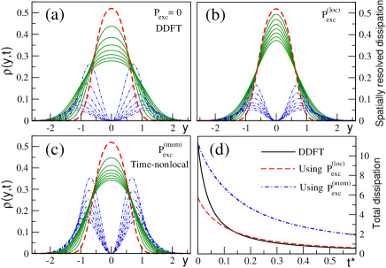
Figure 1: Relaxation of a density peak (slab geometry) from an initial state (red dashed) for which the density is confined to a parabolic potential. Solid green curves show the density and blue dash-dotted curves show the spatially resolved dissipation (scaled down by a factor 20) for three approximations to the excess dissipation (at dimensionless times $t^{*}\!\equiv tk_{\rm B}T/\gamma d^{2}\!\!=\!0.2$ to $1.4$ in steps of $0.2$). Using (a) DDFT, (b) (41), (c) (43). (d) Decay of the total dissipated power.

II.9 Approximations to the excess dissipation

Any practical application of the framework, i.e. implementation of (36) along with (9), requires one to choose an approximation for $P_{t}^{\rm exc}[\rho,{\bf J}]$ for the given physical system (as characterized by $U$). Here we discuss several physically reasonable approximations to $P_{t}^{\rm exc}[\rho,{\bf J}]$, which may be applied to treat systems with arbitrary pairwise interactions. The simplest of these is given by the space- and time-local expression

$$P_{t}^{\rm loc}[\rho,{\bf J}]=\int d{\mathbf{r}}\,\left(\tilde{\gamma}(\rho)-\gamma\right)\frac{{\bf J}({\mathbf{r}},t)^{2}}{2\rho({\mathbf{r}},t)},$$ (41)

where $\tilde{\gamma}(\rho)$ is a density-dependent friction factor which can be approximated using either a virial expansion or, in the case of hard spheres, by employing closed form expressions hayakawa95 . Using (41) slows the dynamics in regions of high density relative to DDFT royallSedimentation , but will still fail to describe collision induced dissipation arising from shearing motions in the fluid. To capture this requires a nonlocal treatment in space and in time which recognizes the finite range of the colloidal interactions. A suitably general form is given by

$$\!\!\!\!P_{t}^{\rm nloc}[\rho,{\bf J}]=\!\!\int\!\!d{\mathbf{r}}\!\!\int\!\!d{\mathbf{r}}^{\prime}\!\!\!\int_{t_{0}}^{t}\!\!\!dt^{\prime}\,{\bf J}({\mathbf{r}},t)\cdot{\bf K}({\mathbf{r}},t;{\mathbf{r}}^{\prime},t^{\prime})\cdot{\bf J}({\mathbf{r}}^{\prime},t^{\prime}),$$ (42)

where the convolution kernel ${\bf K}$ is a second-rank tensor describing current-current scattering and is in general a functional of $\rho$. The incorporation of temporal nonlocality represents a powerful feature of the present approach. A simple specific form for the scattering kernel which captures this is ${\bf K}=\gamma m(t-t^{\prime})\delta({\mathbf{r}}-{\mathbf{r}}^{\prime})/\rho({\mathbf{r}},t)$, where $m(t-t^{\prime})$ is a memory function (with units of inverse time). As a result we obtain a spatially local excess dissipation functional with temporal memory, given by

$$P_{t}^{\rm mem}[\rho,{\bf J}]=\int d{\mathbf{r}}\int_{t_{0}}^{t}dt^{\prime}\frac{\gamma{\bf J}({\mathbf{r}},t)\cdot{\bf J}({\mathbf{r}},t^{\prime})}{\rho({\mathbf{r}},t)}m(t-t^{\prime}).$$ (43)

For general interactions and time-dependent external fields the memory need not be time translationally invariant, as assumed here. The equation of motion (36) thus becomes

$$\frac{\gamma}{\rho({\mathbf{r}},t)} \left({\bf J}({\mathbf{r}},t)+\int_{t_{0}}^{t}dt^{\prime}{\bf J}({\mathbf{r}},t^{\prime})m(t-t^{\prime})\right)=$$

$$-\nabla\frac{\delta F[\rho]}{\delta\rho({\mathbf{r}},t)}-\nabla V_{\rm ext}({\mathbf{r}},t)+{\bf X}({\mathbf{r}},t),$$ (44)

which captures the history-dependence of the one-body current, but neglects the spatial nonlocality of the dissipation.

II.10 Memory effects: A numerical test

We have performed numerical calculations using the (three-dimensional) hard sphere system in a slab geometry using approximations (41) and (43). The (spatially non-local) Rosenfeld functional Rosenfeld89 was used to approximate $F_{\rm exc}[\rho]$. The system is initially confined along the $y$-axis by a parabolic potential, $V_{\rm ext}({\mathbf{r}},t<0)=by^{2}/2$, where $b$ is a constant measuring the strength of the trapping potential. We then switch off the confinement at $t=t_{0}=0$, such that $V_{\rm ext}({\mathbf{r}},t>0)=0$, and monitor the time evolution of the density. In Fig.1 we show the density calculated using three approximations: DDFT, the density-dependent friction coefficient (41) (where we have employed the expression for $\tilde{\gamma}(\rho)$ from hayakawa95 , and the temporally nonlocal approximation (43). When implementing (43) we have approximated the memory function by the simple form $m(t-t^{\prime})=(a/\tau)\exp(-(t-t^{\prime})/\tau)$, where $a$ is a dimensionless parameter and $\tau$ is a relaxation time. In view of the complexity of mode-coupling-type memory functions sjoegren it is clear that the assumption of exponential decay represents a strong simplification, but nevertheless provides a first step towards recognizing the history dependence of the one-body fields.

The density profiles in Fig.1 (generated using the parameter values $a\!=\!0.8,b\!=\!10k_{\rm B}T,\tau\!=\!0.05\gamma d^{2}/k_{\rm B}T$, where the particle diameter, $d$, sets the length-scale) show that both (41) and (43) slow the dynamics. The magnitude of the retardation achieved using (43) depends upon the choice of parameters $a$ and $\tau$ determining the memory. While (43) generates density profiles with a similar functional form to those from DDFT, Eq. (41) leads to a density more sharply peaked at the origin. The spatially resolved dissipation (blue dash-dotted curves) confirms the intuition that power is dissipated mostly in regions of high density gradient and the spatial integral of this quantity, $\int\!d{\mathbf{r}}\,{\bf J}({\mathbf{r}},t)\cdot\delta P_{t}[\rho,{\bf J}]/\delta{\bf J}({\mathbf{r}},t)$, decays towards zero as the system approaches equilibrium. It is well known that relaxation rates predicted by standard DDFT are significantly faster than those found in simulation marinibettolomarconi99 ; royallSedimentation . From our findings we conclude that this failing can be remedied by the incorporation of temporal nonlocality in the excess dissipation functional, leading to memory effects in the equation of motion for ${\bf J}({\mathbf{r}},t)$. If an exponential memory is employed then the computational demands are comparable to those of DDFT.

III Conclusions

In summary, we have shown that collective Brownian dynamics can be formulated as a variational theory (19) based upon the dissipative power as a functional of the one-body density and the one-body current. The underlying many-body expression (11) is a difference of half of the power that is dissipated due to friction and the total power that is generated by the deterministic and entropic forces. As we have shown, this free power functional is minimal for the physical time evolution, and hence plays a role analogous to that of the free energy functional in equilibrium. Thermodynamic potentials in equilibrium are abstract quantities, detectable only through their derivatives. The same is true for the power functional, cf. the equation of motion (32), which hence attains a similar status, but is of more general nature, as it applies out of equilibrium. We have formulated the theory in the Smoluchowski picture, starting with the time evolution of the many-body probability distribution $\Psi({\bf r}^{N}\!\!,t)$. An alternative derivation could be based upon the Langevin equation (1), using the path integral approach to obtain averaged quantities onsager . In both cases, the one-body current and density are averages that do not fluctuate, despite any formal similarities of our approach to dynamical field theories, where the fields themselves can fluctuate.

The appeal of our approach stems from its utility and and ease with which it can be implemented, which contrast strongly with the time-dependent classical DFT formalism by Chan and Finken chan05 . As far as we are aware, the approach of chan05 has never been applied to any model system, possibly because it is built around an action functional, which so far could not be approximated in any systematic or physically intuitive way. This is not the case with the excess dissipation functional identified in the present work, for which even simple expressions, such as (43), transcend the adiabatic approximation. While DDFT remains an active field of research (e.g. hydrodynamic interactions serafim12 and arbitrary particle shapes wittkowski12 have very recently been addressed), it is important to appreciate that all extensions and modifications proposed since the original presentation of DDFT evans79 have been firmly under the constraint of adiabaticity. The power functional approach is free of this restriction and provides a solid, nonadiabatic basis for extensions aiming to treat more complex model systems (e.g. orientational degrees of freedom). Moreover, it applies also to systems governed by many-body forces, where $U({\mathbf{r}}^{N})$ also contains three- and higher-body contributions. The only other nonadiabatic approach of which we are aware is the Generalized Langevin theory of M. Medino-Noyola and coworkers magdeleno . Exploring connections to this work may prove fruitful.

Regarding extensions of the power functional theory: Firstly, generalization to mixtures of different species is straightforward. The ideal contribution becomes $\sum_{i}P_{t}^{\rm id}[\rho_{i},{\bf J}_{i}]$, where $i$ enumerates the different species, whereas the excess dissipation, $P_{t}^{\rm exc}[\{\rho_{i}\},\{{\bf J}_{i}\}]$, generates dynamical coupling between particles of different species. Secondly, if the Langevin equation (1) is generalized to include a velocity-dependent friction coefficient, $\gamma({\bf v}_{i}(t))$, a modified version of the ideal dissipation functional applies, $P_{t}^{\rm id,nl}[\rho,{\bf J}]=\int d{\mathbf{r}}\rho({\mathbf{r}},t)f({\bf v}({\mathbf{r}},t)^{2})$, where the function $f(\cdot)$ is related to the density-dependent friction force via $\gamma({\bf v}^{2})=2\rho f^{\prime}({\bf v}^{2})$ and the prime denotes differentiation with respect to the argument.

Much of the phenomenology of non-equilibrium dynamics can be investigated using two- and higher-body correlation functions. Using the dynamical test particle method archer07dtpl , which identifies the van Hove function with the dynamics of suitably constructed one-body fields, one has immediate access within the present framework to the dynamic structure factor and the intermediate scattering function. Moreover, the relationships (26) and (27) of the one-body fields to their generating functional imply that two- and higher-body dynamic correlation functions can be generated from further functional differentiation, putting a non-equilibrium generalization of the Ornstein-Zernike relation, which in equilibrium is a cornerstone of liquid state theory hansen , within reach. Work along these lines, as well as application to driven lattice models dwandaru , is currently in progress.

- (1) J. K. G. Dhont, An introduction to dynamics of colloids (Elsevier, Amsterdam, 1996).
- (2) J. Mewis and N. J. Wagner, Colloidal suspension rheology (Cambridge University Press, Cambridge, 2012).
- (3) J. M. Brader, J. Phys.: Condensed Matter 22, 363101 (2010).
- (4) R. Evans, Adv. Phys. 28 143 (1979).
- (5) U. M. B. Marconi and P. Tarazona, J. Chem. Phys. 110, 8032 (1999).
- (6) P. Español and H. Löwen, J. Chem. Phys. 131, 244101 (2009).
- (7) A. J. Archer and R. Evans, J. Chem. Phys. 121, 4246 (2004).
- (8) W. Götze and L. Sjögren, Rep. Prog. Phys. 55, 241 (1992).
- (9) J. Reinhardt and J. M. Brader, EPL 102, 28011 (2013).
- (10) J. M. Brader and M. Krüger, Mol. Phys. 109, 1029 (2011).
- (11) D. R. Foss and J. F. Brady, J. Rheol. 44, 629 (2000).
- (12) X. Xu, S. Rice and A. R. Dinner, Proc. Natl. Acad. Sci. 110, 3771 (2013).
- (13) M. Frank, D. Anderson, E. R. Weeks and J. F. Morris, J. Fluid. Mech. 493, 363 (2003).
- (14) H. Riskin, The Fokker-Planck Equation, (Springer, Berlin, 1989).
- (15) E. Runge and E. K. U. Gross, Phys. Rev. Lett. 52, 997 (1984); A. K. Dhara and S. K. Ghosh, Phys. Rev. A 35, 442 (1987).
- (16) H. Goldstein, C. Poole, and J. Safko, Classical Mechanics (Addison Wesley, San Francisco, 2002).
- (17) N. D. Mermin, Phys. Rev. 137, A1441 (1965).
- (18) P. Hohenberg and W. Kohn, Phys. Rev. 136, B864 (1964).
- (19) M. Levy, Proc. Natl. Acad. Sci. 76, 6062 (1979); see also J. K. Percus, Int. J. Quant. Chem. 13, 89 (1978).
- (20) W. S. B. Dwandaru and M. Schmidt, Phys. Rev. E 83, 061133 (2011).
- (21) H. Hayakawa and K. Ichiki, Phys. Rev. E 51, R3815 (1995).
- (22) C. P. Royall, J. Dzubiella, M. Schmidt, and A. van Blaaderen, Phys. Rev. Lett. 98, 188304 (2007).
- (23) Y. Rosenfeld, Phys. Rev. Lett. 63, 980 (1989).
- (24) L. Onsager and S. Machlup, Phys. Rev. 91, 1505 (1953).
- (25) G. K. L. Chan and R. Finken, Phys. Rev. Lett. 94, 183001 (2005).
- (26) B. D. Goddard, A. A. Nold, N. N. Savva, G. A. Pavliotis and S. S. Kalliadasis, Phys. Rev. Lett. 109, 120603 (2012).
- (27) R. Wittkowski and H. Löwen, Mol. Phys. 109, 2935 (2011).
- (28) A. J. Archer, P. Hopkins and M. Schmidt, Phys. Rev. E 75, 040501(R) (2007).
- (29) P. Ramirez-Gonzalez and M. Medina-Noyola, Phys. Rev. E 82, 061503 (2010).
- (30) J.-P. Hansen and I. R. McDonald, Theory of Simple Liquids, (Academic press, 1986).
- (31) W. S. B. Dwandaru and M. Schmidt, J. Phys. A: Math. Theo. 40, 13209 (2007).