Left-orderable fundamental group and Dehn surgery on genus one two-bridge knots

Abstract.

For any hyperbolic genus one $2$-bridge knot in the $3$-sphere, we show that the resulting manifold by $r$-surgery on the knot has left-orderable fundamental group if the slope $r$ lies in some range which depends on the knot.

1. Introduction

A non-trivial group $G$ is said to be left-orderable if it admits a strict total ordering which is invariant under left-multiplication. Thus, if $g<h$ then $fg<fh$ for any $f,g,h\in G$. Many fundamental groups of $3$-manifolds are known to be left-orderable. For examples, all knot and link groups are left-orderable. Boyer, Gordon and Watson [3] propose a conjecture that an irreducible rational homology $3$-sphere $Y$ is an $L$-space if and only if $\pi_{1}Y$ is not left-orderable. An $L$-space is a rational homology $3$-sphere whose Heegaard–Floer homology $\widehat{HF}(Y)$ has rank $|H_{1}(Y;\mathbb{Z})|$ ([16]). Recently, $L$-spaces become the object of interest, and it is an open problem to characterize $L$-spaces without mentioning Heegaard–Floer homology. The affirmative answer to the above conjecture will give an algebraic characterization of $L$-spaces.

On the other hand, irreducible rational homology spheres are obtained by Dehn surgery on knots in the $3$-sphere $S^{3}$, in plenty. For a knot $K$, we call a slope $r$ left-orderable if the resulting manifold $K(r)$ by $r$-surgery on $K$ has left-orderable fundamental group. In this paper, a slope is sometimes identified with its parameter in $\mathbb{Q}\cup\{1/0\}$. In particular, the meridional slope corresponds to $1/0$. It is known that any hyperbolic $2$-bridge knot does not admit Dehn surgery yielding an $L$-space ([16]). Hence any slope but $1/0$ is expected to be left-orderable for a hyperbolic $2$-bridge knot, if we support the above conjecture. In this direction, Boyer, Gordon and Watson [3] proved that for the figure-eight knot, if $r\in(-4,4)$, then $r$ is left-orderable. Later, Clay, Lidman and Watson [6] showed $r=\pm 4$ are also left-orderable. These results were extended to all hyperbolic twist knots [10, 11, 19]. Also, Tran [20] further extended the range of left-orderable slopes for twist knots.

The purpose of this paper is to give new ranges of left-orderable slopes for all hyperbolic genus one, $2$-bridge knots. As a by-product, we obtain a wider range of left-orderable slopes for (positive) twist knots than that in [11].

For non-zero integers $m$ and $n$, let $K(m,n)$ be the $2$-bridge knot $S(4mn+1,2m)$ in Schubert’s normal form as illustrated in Figure 1. In Figure 1, the twists in the vertical box are left-handed (resp. right-handed) if $m>0$ (resp. $m<0$), but those in the horizontal box are right-handed (resp. left-handed) if $n>0$ (resp. $n<0$). Thus $K(1,-1)$ is the trefoil, and $K(1,1)$ is the figure-eight knot. By symmetry, $K(m,n)$ and $K(-n,-m)$ are isotopic. Except the trefoil, $K(m,n)$ is hyperbolic. It is also well known that any genus one $2$-bridge knot is equivalent to $K(m,n)$ for some $m,n$ (see [5]).

Figure 1. The knot $K(m,n)$

Theorem 1.1.

Let $K=K(m,n)$ be a hyperbolic genus one $2$-bridge knot $S(4mn+1,2m)$ in the $3$-sphere $S^{3}$ as illustrated in Figure 1. Let $I$ be the interval defined by

$$I=\begin{cases}(-4n,4m)&\text{if $m>0$ and $n>0$},\\ (4m,-4n)&\text{if $m<0$ and $n<0$},\\ [0,\max\{4m,-4n\})&\text{if $m>0$ and $n<0$},\\ (\min\{4m,-4n\},0]&\text{if $m<0$ and $n>0$}.\end{cases}$$

Then any slope in $I$ is left-orderable. That is, $\pi_{1}(K(r))$ is left-orderable.

We remark that $K(1,-1)$ and $K(-1,1)$ are trefoils, so they are excluded in the statement here.

In a previous paper [11], we showed that any hyperbolic twist knot $K(1,n)\ (n\neq-1)$ admits a range $[0,4]$ of left-orderable slopes. Theorem 1.1 gives a partial improvement of this result.

Corollary 1.2.

Let $K=K(1,n)$ be a hyperbolic $n$-twist knot for $n>0$. If $I=(-4n,4]$, then any slope in $I$ is left-orderable.

This range of Corollary 1.2 coincides with that in [20]. Also, Tran informed us that he obtained a similar result to Theorem 1.1. We would like to thank Anh T. Tran for informing his result.

2. Knot groups and Two sequences of polynomials

Let $K=K(m,n)$ and let $G=\pi_{1}(S^{3}-K)$ be its knot group. We always assume that $m\neq 0$ and $n\neq 0$, unless specified otherwise.

Proposition 2.1.

The knot group $G$ admits a presentation

$$G=\langle x,y\mid w^{n}x=yw^{n}\rangle,$$

where $x$ and $y$ are meridians and $w=(xy^{-1})^{m}(x^{-1}y)^{m}$. Furthermore, the longitude $\mathcal{L}$ is given as $\mathcal{L}=w_{*}^{n}w^{n}$, where $w_{*}=(yx^{-1})^{m}(y^{-1}x)^{m}$ is obtained from $w$ by reversing the order of letters.

This is slightly different from that in [13, Proposition 1], but both are isomorphic.

Proof.

We use a surgery diagram of $K$ as illustrated in Figure 2, where $1/m$–surgery and $-1/n$–surgery are performed along the second and third components, respectively. Let $\mu_{i}$ and $\lambda_{i}$ be the meridian and longitude of the $i$th component.

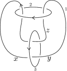
Figure 2. A surgery diagram of $K$

First, $y=\mu_{3}^{-1}x\mu_{3}$, $z=\mu_{2}^{-1}y\mu_{2}$, $\lambda_{2}=x^{-1}y$ and $\lambda_{3}=yz^{-1}$. By $1/m$–surgery on the second component yields a relation $\lambda_{2}^{m}\mu_{2}=1$, so $\mu_{2}=\lambda_{2}^{-m}$. Similarly, $-1/n$–surgery on the third component gives $\mu_{3}=\lambda_{3}^{n}$. Thus

$$\lambda_{3} = y\mu_{2}^{-1}y^{-1}\mu_{2}=y\lambda_{2}^{m}y^{-1}\lambda_{2}^{-m}$$

$$= y(x^{-1}y)^{m}y^{-1}(y^{-1}x)^{m}=(yx^{-1})^{m}(y^{-1}x)^{m}.$$

Then the relation $y=\mu_{3}^{-1}x\mu_{3}$ gives

(2.1) $$y[(x^{-1}y)^{m}(xy^{-1})^{m}]^{n}=[(x^{-1}y)^{m}(xy^{-1})^{m}]^{n}y.$$

Set $w=(xy^{-1})^{m}(x^{-1}y)^{m}$. Since $[(x^{-1}y)^{m}(xy^{-1})^{m}]^{n}=(x^{-1}y)^{m}w^{n}(x^{-1}y)^{-m}$, (2.1) changes to $y(x^{-1}y)^{m}w^{n}(x^{-1}y)^{-m}=(x^{-1}y)^{m}w^{n}(x^{-1}y)^{-m}x$. By $y(x^{-1}y)^{m}=(yx^{-1})^{m}y$, we have $(yx^{-1})^{m}yw^{n}(x^{-1}y)^{-m}=(x^{-1}y)^{m}w^{n}(x^{-1}y)^{-m}x$. Thus,

$$yw^{n} = (xy^{-1})^{m}(x^{-1}y)^{m}w^{n}(x^{-1}y)^{-m}x(x^{-1}y)^{m}$$

$$= w^{n+1}(x^{-1}y)^{-m}x(x^{-1}y)^{m}$$

$$= w^{n}(xy^{-1})^{m}(x^{-1}y)^{m}(x^{-1}y)^{-m}x(x^{-1}y)^{m}$$

$$= w^{n}(xy^{-1})^{m}x(x^{-1}y)^{m}$$

$$= w^{n}x.$$

Set $w_{*}=(yx^{-1})^{m}(y^{-1}x)^{m}$. Then $\lambda_{3}=w_{*}$. The longitude is $\mathcal{L}=\mu_{3}\mu_{2}\mu_{3}^{-1}\mu_{2}^{-1}=w_{*}^{n}\mu_{2}w_{*}^{-n}\mu_{2}^{-1}$. We have

$$\mu_{2}w_{*}^{-n}\mu_{2}^{-1} = (x^{-1}y)^{-m}[(yx^{-1})^{m}(y^{-1}x)^{m}]^{-n}(x^{-1}y)^{m}$$

$$= (x^{-1}y)^{-m}[(x^{-1}y)^{m}(xy^{-1})^{m}]^{n}(x^{-1}y)^{m}$$

$$= [(xy^{-1})^{m}(x^{-1}y)^{m}]^{n}$$

$$= w^{n}.$$

Thus $\mathcal{L}=w_{*}^{n}w^{n}$. ∎

To describe the Riley polynomial of $K$ in Section 3, we prepare two sequences of polynomials with a single variable $s$.

For non-negative integer $m$, let $f_{m}\in\mathbb{Z}[s]$ be defined by the recursion

(2.2) $$f_{m+2}-(s+2)f_{m+1}+f_{m}=0$$

with initial conditions $f_{0}=1$ and $f_{1}=s+1$. Also, let $g_{m}\in\mathbb{Z}[s]$ be defined by the same recursion

(2.3) $$g_{m+2}-(s+2)g_{m+1}+g_{m}=0$$

with slightly different initial conditions $g_{0}=1$ and $g_{1}=s+2$. We remark that $g_{m}$ is equivalent to the Chebyshev polynomial of the second kind.

Lemma 2.2.

The closed formulas for $f_{m}$ and $g_{m}$ are

$$f_{m}=\sum_{i=0}^{m}\binom{m+i}{m-i}s^{i},\quad g_{m}=\sum_{i=0}^{m}\binom{m+1+i}{m-i}s^{i}.$$

In particular, all coefficients of $f_{m}$ and $g_{m}$ are positive integers, and the degree of $f_{m}$ and $g_{m}$ is $m$. Also, $f_{m}$ and $g_{m}$ are monic.

Proof.

These easily follow from the inductive argument by using the recursive formulas. ∎

Set $f_{-m}=f_{m-1}$ for $m\geq 1$, and set $g_{-1}=0$ and $g_{-m}=-g_{m-2}$ for $m\geq 2$. Thus we have defined $f_{m}$ and $g_{m}$ for any integer $m$. In particular, the recursions (2.2) and (2.3) hold for all integers.

Lemma 2.3.

For any integer $m$, the polynomials $f_{m}$, $g_{m}$ satisfy the following relations.

• $f_{m}+g_{m-1}=g_{m}$.

• $f_{m}+sg_{m}=f_{m+1}$.

• $f_{m}^{2}=sg_{m}g_{m-1}+1$.

Proof.

These are easily proved by induction. We prove (3) only here. Clearly, it holds when $m=0$. Assume $f_{m}^{2}=sg_{m}g_{m-1}+1$. From (1) and (2),

$$f_{m+1}^{2} = (f_{m}+sg_{m})^{2}$$

$$= f_{m}^{2}+2sf_{m}g_{m}+s^{2}g_{m}^{2}$$

$$= (sg_{m}g_{m-1}+1)+2sf_{m}g_{m}+s^{2}g_{m}^{2}$$

$$= (sg_{m}g_{m-1}+1)+2s(g_{m}-g_{m-1})g_{m}+s^{2}g_{m}^{2}$$

$$= (s^{2}+2s)g_{m}^{2}-sg_{m}g_{m-1}+1$$

$$= s((s+2)g_{m}-g_{m-1})g_{m}+1$$

$$= sg_{m+1}g_{m}+1.$$

Similarly, $f_{m-1}^{2}=(f_{m}-sg_{m-1})^{2}=sg_{m-1}g_{m-2}+1$. ∎

Lemma 2.4.

If a positive real number is substituted to $s$, then we have the following inequalities.

• For $m>0$, $sg_{m-1}<4f_{m}$.

• For $m<0$, $-sg_{m-1}<4f_{m-1}$.

• For $m<0$, $-2sg_{m-1}<3f_{m-1}$.

Proof.

(1) Since $sg_{m-1}=f_{m}-f_{m-1}$ by Lemma 2.3, this follows from $3f_{m}+f_{m-1}>0$. (2) is equivalent to (1). (3) From $sg_{m-1}=f_{m}-f_{m-1}$, it follows from $2f_{m}+f_{m-1}>0$. ∎

3. Riley polynomials

In this section, we calculate the Riley polynomial of $K$. Let $s$ and $t$ be real numbers such that $s>0$ and $t>1$. Let $\rho:G\to SL_{2}(\mathbb{R})$ be a representation of $G$ defined by

$$\rho(x)=\begin{pmatrix}\sqrt{t}&1/\sqrt{t}\\ 0&1/\sqrt{t}\\ \end{pmatrix},\quad\rho(y)=\begin{pmatrix}\sqrt{t}&0\\ -s\sqrt{t}&1/\sqrt{t}\\ \end{pmatrix}.$$

By [17], $\rho$ gives a non-abelian representation if $s$ and $t$ are a pair of solutions of the Riley polynomial. Recall that $w=(xy^{-1})^{m}(x^{-1}y)^{m}$. Let $W=\rho(w)$ and $z_{i,j}$ be the $(i,j)$-entry of $W^{n}$. Then the Riley polynomial of $K$ is given by $\phi_{K}(s,t)=z_{1,1}+(1-t)z_{1,2}$. (See also [8].)

Since $s$ and $t$ are limited to be positive real numbers in our setting, it is not obvious that there exist solutions for Riley’s equation $\phi_{K}(s,t)=0$. However, this will be verified in Proposition 4.2 under some condition. In fact, we can choose $t$ so that $t>1$ and $s+2<t+1/t<s+2+4/(sg_{m-1}^{2})$ for any $s>0$. We temporarily assume that $s$ and $t$ are chosen to satisfy $\phi_{K}(s,t)=0$. See Example 3.7 when $n=\pm 1$.

Proposition 3.1.

For $W=\rho(w)$, we have

$$W=\begin{pmatrix}f_{m}^{2}-stg_{m-1}^{2}&f_{m-1}g_{m-1}-\frac{f_{m}g_{m-1}}{t}\\ sf_{m}g_{m-1}-stf_{m-1}g_{m-1}&f_{m-1}^{2}-\frac{s}{t}g_{m-1}^{2}\end{pmatrix}.$$

Proof.

We prove by induction on $m$. (For the knot $K(m,n)$, we assume $m\neq 0$. However, this proposition holds even for $m=0$.)

If $m=0$, then $w=1$, so $W$ is the identity matrix. It is easy to check that the claim holds.

Assume the conclusion for $m$. Note

$$\rho(xy^{-1})=\begin{pmatrix}s+1&1\\ s&1\end{pmatrix},\ \rho(x^{-1}y)=\begin{pmatrix}s+1&-1/t\\ -st&1\end{pmatrix}.$$

Calculate the product

$$\begin{pmatrix}s+1&1\\ s&1\end{pmatrix}\begin{pmatrix}f_{m}^{2}-stg_{m-1}^{2}&f_{m-1}g_{m-1}-\frac{f_{m}g_{m-1}}{t}\\ sf_{m}g_{m-1}-stf_{m-1}g_{m-1}&f_{m-1}^{2}-\frac{s}{t}g_{m-1}^{2}\end{pmatrix}\begin{pmatrix}s+1&-1/t\\ -st&1\end{pmatrix}.$$

By using Lemma 2.3, each entry is identified as desired. For example, the $(1,1)$-entry is

$$(f_{m}+s(f_{m}+g_{m-1}))^{2}-st(f_{m-1}+g_{m-1}+sg_{m-1})^{2} = (f_{m}+sg_{m})^{2}-st(f_{m-1}+(s+1)g_{m-1})^{2}$$

$$= f_{m+1}^{2}-st(f_{m}+g_{m-1})^{2}$$

$$= f_{m+1}^{2}-stg_{m}^{2}.$$

Similarly,

$$\rho(yx^{-1})=\begin{pmatrix}1&-1\\ -s&s+1\end{pmatrix},\ \rho(y^{-1}x)=\begin{pmatrix}1&1/t\\ st&s+1\end{pmatrix}.$$

Then, calculating the product

$$\begin{pmatrix}1&-1\\ -s&s+1\end{pmatrix}\begin{pmatrix}f_{m}^{2}-stg_{m-1}^{2}&f_{m-1}g_{m-1}-\frac{f_{m}g_{m-1}}{t}\\ sf_{m}g_{m-1}-stf_{m-1}g_{m-1}&f_{m-1}^{2}-\frac{s}{t}g_{m-1}^{2}\end{pmatrix}\begin{pmatrix}1&1/t\\ st&s+1\end{pmatrix}$$

gives the conclusion again. ∎

Let $\lambda_{\pm}\in\mathbb{C}$ be the eigenvalues of $W$.

Lemma 3.2.

$\lambda_{+}\neq\lambda_{-}$.

Proof.

Since $\det W=1$, $\lambda_{+}\lambda_{-}=1$. If $\lambda_{+}=\lambda_{-}$, then $\lambda_{+}=\lambda_{-}=\pm 1$. Then $\mathrm{tr}W=\pm 2$.

On the other hand, $\mathrm{tr}W=f_{m}^{2}+f_{m-1}^{2}-s(t+1/t)g_{m-1}^{2}=s(s+2-t-1/t)g_{m-1}^{2}+2$ by Proposition 3.1 and Lemma 2.3. Since $g_{m-1}\neq 0$, $s>0$ and $s+2<t+1/t$, $\mathrm{tr}W<2$. If $\mathrm{tr}W=-2$, then $s(t+1/t-s-2)g_{m-1}^{2}=4$, so $t+1/t=s+2+4/(sg_{m-1}^{2})$. But this is impossible by our choice of $t$, remarked before Proposition 3.1. Hence $\lambda_{+}\neq\lambda_{-}$. ∎

Let $w_{i,j}$ be the $(i,j)$-entry of $W$, and let $P=\begin{pmatrix}w_{1,2}&w_{1,2}\\ \lambda_{+}-w_{1,1}&\lambda_{-}-w_{1,1}\end{pmatrix}$.

Lemma 3.3.

$w_{1,2}\neq 0$.

Proof.

Assume $w_{1,2}=0$. By Proposition 3.1, $w_{1,2}=f_{m-1}g_{m-1}-f_{m}g_{m-1}/t$. Since $m\neq 0$, $g_{m-1}\neq 0$. Hence $f_{m}=tf_{m-1}$.

From the recursion (2.2), $tf_{m-1}-(s+2)f_{m-1}+f_{m-2}=0$. Since $f_{m-1}\neq 0$, we have $t=s+2-f_{m-2}/f_{m-1}$. Thus $t<s+2$, contradicting our choice of $t$ again. ∎

The next will be used in Section 5.

Lemma 3.4.

$w_{2,1}=-stw_{1,2}$. Hence $w_{2,1}\neq 0$.

Proof.

This immediately follows from Proposition 3.1 and Lemma 3.3. ∎

By Lemmas 3.2 and 3.3, $\det P=-w_{1,2}(\lambda_{+}-\lambda_{-})\neq 0$. A direct calculation shows $P^{-1}WP=\begin{pmatrix}\lambda_{+}&0\\ 0&\lambda_{-}\end{pmatrix}$.

Set $\tau=\mathrm{tr}W$. For any positive integer $k$, let $\tau_{k}=\tau^{k-1}+\tau^{k-3}+\dots+\tau^{3-k}+\tau^{1-k}$. If $\lambda_{+}\neq\lambda_{-}$, then $\tau_{k}=(\lambda_{+}^{k}-\lambda_{-}^{k})/(\lambda_{+}-\lambda_{-})$. Let $\tau_{0}=0$ and $\tau_{-k}=-\tau_{k}$. Then a recursion $\tau_{k+1}-\tau\tau_{k}+\tau_{k-1}=0$ holds for any integer $k$.

Lemma 3.5.

For $W^{n}=\rho(w^{n})$, we have

$$W^{n}=\begin{pmatrix}w_{1,1}\tau_{n}-\tau_{n-1}&w_{1,2}\tau_{n}\\ w_{2,1}\tau_{n}&\tau_{n+1}-w_{1,1}\tau_{n}\end{pmatrix}.$$

Proof.

When $n=\pm 1$, it is easy to see the conclusion. Let $|n|>1$. This easily follows from $W^{n}=P\begin{pmatrix}\lambda_{+}^{n}&0\\ 0&\lambda_{-}^{n}\end{pmatrix}P^{-1}$. ∎

Proposition 3.6.

The Riley polynomial of $K$ is

$$\phi_{K}(s,t)=(\tau_{n+1}-\tau_{n})+(s+2-t-1/t)f_{m-1}g_{m-1}\tau_{n}.$$

Proof.

By [17] (see also [8, p.309]), the Riley polynomial is $\phi_{K}(s,t)=z_{1,1}+(1-t)z_{1,2}$, where $z_{i,j}$ is the $(i,j)$-entry of $W^{n}$. From Lemma 3.5 and the recursive formula for $\tau_{k}$,

$$\phi_{K}(s,t) = (w_{1,1}\tau_{n}-\tau_{n-1})+(1-t)w_{1,2}\tau_{n}$$

$$= \tau_{n+1}-(\mathrm{tr}W)\tau_{n}+(w_{1,1}+(1-t)w_{1,2})\tau_{n}$$

$$= (\tau_{n+1}-\tau_{n})+(w_{1,1}+(1-t)w_{1,2}+1-\mathrm{tr}W)\tau_{n}.$$

By Proposition 3.1, $\mathrm{tr}W=f_{m}^{2}+f_{m-1}^{2}-s(t+1/t)g_{m-1}^{2}$. Thus we have

$$w_{1,1}+(1-t)w_{1,2}+1-\mathrm{tr}W=(2-t-1/t)f_{m-1}g_{m-1}+1-f_{m-1}^{2}+sg_{m-1}^{2}.$$

Since

$$1-f_{m-1}^{2}+sg_{m-1}^{2} = -sg_{m-1}g_{m-2}+sg_{m-1}^{2}$$

$$= sg_{m-1}(g_{m-1}-g_{m-2})$$

$$= sg_{m-1}f_{m-1},$$

we obtain $\phi_{K}(s,t)=(\tau_{n+1}-\tau_{n})+(s+2-t-1/t)f_{m-1}g_{m-1}\tau_{n}$. ∎

For convenience, we introduce a variable $T=t+1/t$. Then the Riley polynomial of $K$ is expressed as $\phi_{K}(s,T)=(\tau_{n+1}-\tau_{n})+(s+2-T)f_{m-1}g_{m-1}\tau_{n}$.

We remark that the Riley polynomial of $K$ is also described by [15] in a different form.

Example 3.7.

If $n=1$, then

$$\phi_{K}(s,T) = (\tau_{2}-\tau_{1})+(s+2-T)f_{m-1}g_{m-1}\tau_{1}$$

$$= (\mathrm{tr}W-1)+(s+2-T)f_{m-1}g_{m-1}$$

$$= s(s+2-T)g_{m-1}^{2}+1+(s+2-T)f_{m-1}g_{m-1}$$

$$= (s+2-T)g_{m-1}(sg_{m-1}+f_{m-1})+1$$

$$= (s+2-T)g_{m-1}f_{m}+1.$$

Thus Riley’s equation $\phi_{K}(s,T)=0$ has the unique solution $T=s+2+1/(f_{m}g_{m-1})$ for any $s>0$. If $m>0$, then $T>s+2>2$, because $f_{m}>0$ and $g_{m-1}>0$. Hence we have a real solution $t=(T+\sqrt{T^{2}-4})/2>1$. By Lemma 2.4(1), we also have $s+2<T<s+2+4/(sg_{m-1}^{2})$.

If $n=-1$, then $\phi_{K}(s,T)=1+(T-s-2)f_{m-1}g_{m-1}$. Hence the equation $\phi_{K}(s,T)=0$ also has the unique solution $T=s+2-1/(f_{m-1}g_{m-1})$. If $m<0$, then $T>s+2>2$, so there exists a real solution $t>1$ as above. Again, $s+2<T<s+2+4/(sg_{m-1}^{2})$ by Lemma 2.4(2).

4. Solutions of Riley’s equation

In this section, we examine when Riley’s equation $\phi_{K}(s,T)=0$ has a pair of real solutions $(s,T)$. In fact, we can choose $T$ satisfying $s+2+c/s<T<s+2+d/s$, where $c$ and $d$ are constants depending only $n$, for any $s>0$, unless $n=\pm 1$.

Let $k$ be a positive integer. For $z=e^{i\theta}$ $(0\leq\theta\leq\pi)$, set $\mathcal{T}_{k}(z)=z^{k-1}+z^{k-3}+\dots+z^{3-k}+z^{1-k}$. If $z\neq\pm 1$, then $\mathcal{T}_{k}(z)=(z^{k}-z^{-k})/(z-z^{-1})$. Define $\mathcal{T}_{0}=0$ and $\mathcal{T}_{-k}(z)=-\mathcal{T}_{k}(z)$. Since $\mathcal{T}_{k}(z)$ is symmetric for $z$ and $z^{-1}$, it can be expanded as a polynomial of $z+z^{-1}$. Furthermore, a recursive relation

$$\mathcal{T}_{k+1}(z)-(z+z^{-1})\mathcal{T}_{k}(z)+\mathcal{T}_{k-1}(z)=0$$

holds. Also, $\mathcal{T}_{k}(1)=k$ and $\mathcal{T}_{k}(-1)=(-1)^{k-1}k$ for any integer $k$.

Lemma 4.1.

• Let $k\geq 1$. Then, $\mathcal{T}_{k}(e^{\frac{\pi}{2k+1}i})=\mathcal{T}_{k+1}(e^{\frac{\pi}{2k+1}i})$. This value is positive.

• Let $m\geq 2$. Then, $\mathcal{T}_{k}(e^{\frac{3\pi}{2k+1}i})=\mathcal{T}_{k+1}(e^{\frac{3\pi}{2k+1}i})$. This value is negative.

Proof.

(1) Let $z=e^{\frac{\pi}{2k+1}i}$. Then the fact that $z^{2k+1}=-1$ immediately implies $\mathcal{T}_{k}(z)=\mathcal{T}_{k+1}(z)$. A direct calculation shows

$$\mathcal{T}_{k}(z)=\frac{\sin\frac{k\pi}{2k+1}}{\sin\frac{\pi}{2k+1}}>0.$$

(2) Similarly, set $z=e^{\frac{3\pi}{2k+1}i}$. Then $z^{2k+1}=-1$ holds again. Hence we have $\mathcal{T}_{k}(z)=\mathcal{T}_{k+1}(z)$, and

$$\mathcal{T}_{k}(z)=\frac{\sin\frac{3k\pi}{2k+1}}{\sin\frac{3\pi}{2k+1}}<0.$$

∎

Now, fix an $s>0$. We introduce a function $\Phi:[s+2,s+2+4/(sg_{m-1}^{2})]\to\mathbb{R}$ by

(4.1) $$\Phi(T)=(\mathcal{T}_{n+1}(z)-\mathcal{T}_{n}(z))+(s+2-T)f_{m-1}g_{m-1}\mathcal{T}_{n}(z),$$

where $z=(\tau+i\sqrt{4-\tau^{2}})/2$ with $\tau=s(2+s-T)g_{m-1}^{2}+2$.

Note that $-2\leq\tau\leq 2$. We will seek a solution $T$ for $\Phi(T)=0$ satisfying $s+2<T<s+2+4/(sg_{m-1}^{2})$, because it gives a pair of solutions $(s,T)$ for Riley’s equation $\phi_{K}(s,T)=0$.

Proposition 4.2.

Suppose $n\neq\pm 1$. For any $s>0$, Riley’s equation $\phi_{K}(s,T)=0$ has a solution $T$ satisfying $s+2+c/(sg_{m-1}^{2})<T<s+2+d/(sg_{m-1}^{2})$, where $c$ and $d$ are constants in $(0,4)$ depending only on $n$. In particular, $\phi_{K}(s,t)=0$ has a solution $t>1$ for any $s>0$.

Proof.

Suppose $n>1$. By Lemma 4.1,

$$\mathcal{T}_{n+1}(e^{\frac{\pi}{2n+1}i})=\mathcal{T}_{n}(e^{\frac{\pi}{2n+1}i}),\quad\mathcal{T}_{n+1}(e^{\frac{3\pi}{2n+1}i})=\mathcal{T}_{n}(e^{\frac{3\pi}{2n+1}i}).$$

Let $c=2-2\cos\frac{\pi}{2n+1}$ and $c^{\prime}=2-2\cos\frac{3\pi}{2n+1}$. Then $c,c^{\prime}\in(0,4)$ and $c<c^{\prime}$.

If $T=s+2+c/(sg_{m-1}^{2})$ (resp. $s+2+c^{\prime}/(sg_{m-1}^{2}$) then $\tau=2-c$ (resp. $2-c^{\prime}$). Thus

$$\Phi(s+2+\frac{c}{sg_{m-1}^{2}}) = -\frac{cf_{m-1}}{sg_{m-1}}\mathcal{T}_{n}(e^{\frac{\pi}{2n+1}i}),$$

$$\Phi(s+2+\frac{c^{\prime}}{sg_{m-1}^{2}}) = -\frac{c^{\prime}f_{m-1}}{sg_{m-1}}\mathcal{T}_{n}(e^{\frac{3\pi}{2n+1}i}).$$

By Lemma 4.1, these values have distinct signs. We remark that $\Phi(T)$ is a polynomial function of $T$, so it is continuous. Thus if $n>1$, we have a solution $T$ for $\Phi(T)=0$, satisfying $s+2+c/(sg_{m-1}^{2})<T<s+2+c^{\prime}/(sg_{m-1}^{2})$, from the Intermediate-Value Theorem. Since $T>2$, $t+1/t=T$ has a real solution for $t$. If we choose $t=(T+\sqrt{T^{2}-4})/2$, then $t>1$.

Suppose $n<-1$. Set $l=|n|$. If $l>2$, then set $d=2-2\cos\frac{\pi}{2l-1}$ and $d^{\prime}=2-2\cos\frac{3\pi}{2l-1}$. Then $d,d^{\prime}\in(0,4)$ and $d<d^{\prime}$. As before,

$$\mathcal{T}_{l-1}(e^{\frac{\pi}{2l-1}i})=\mathcal{T}_{l}(e^{\frac{\pi}{2l-1}i}),\quad\mathcal{T}_{l-1}(e^{\frac{3\pi}{2l-1}i})=\mathcal{T}_{l}(e^{\frac{3\pi}{2l-1}i}).$$

by Lemma 4.1. Thus

$$\Phi(s+2+\frac{d}{sg_{m-1}^{2}}) = \frac{d\,f_{m-1}}{sg_{m-1}^{2}}\mathcal{T}_{l}(e^{\frac{\pi}{2l-1}i}),$$

$$\Phi(s+2+\frac{d^{\prime}}{sg_{m-1}^{2}}) = \frac{d^{\prime}f_{m-1}}{sg_{m-1}^{2}}\mathcal{T}_{l}(e^{\frac{3\pi}{2l-1}i}).$$

Since these values have distinct signs, we have a solution $T$ with $s+2+d/(sg_{m-1}^{2})<T<s+2+d^{\prime}/(sg_{m-1}^{2})$, if $l>2$, as before.

When $l=2$, we have

$$\Phi(s+2+\frac{1}{sg_{m-1}^{2}})=\frac{f_{m-1}}{sg_{m-1}},\quad\Phi(s+2+\frac{2}{sg_{m-1}^{2}})=-1,$$

$$\Phi(s+2+\frac{3}{sg_{m-1}^{2}})=-2-\frac{3f_{m-1}}{sg_{m-1}}.$$

If $m>0$, then $\Phi(s+2+1/(sg_{m-1}^{2}))>0$, since $f_{m-1},g_{m-1}>0$. Therefore there exists a solution $T$ with $s+2+1/(sg_{m-1}^{2})<T<s+2+2/(sg_{m-1}^{2})$. If $m<0$, $\Phi(s+2+3/(sg_{m-1}^{2}))>0$, since $3f_{m-1}>-2sg_{m-1}$ by Lemma 2.4(3). Thus there exists a solution $T$ with $s+2+2/(sg_{m-1}^{2})<T<s+2+3/(sg_{m-1}^{2})$ ∎

5. Longitudes

For $s>0$, let $\rho_{s}:G\to SL_{2}(\mathbb{R})$ be the representation defined by the correspondence

(5.1) $$\rho_{s}(x)=\begin{pmatrix}\sqrt{t}&0\\ 0&\frac{1}{\sqrt{t}}\end{pmatrix},\quad\rho_{s}(y)=\begin{pmatrix}\frac{t-s-1}{\sqrt{t}-\frac{1}{\sqrt{t}}}&\frac{s}{(\sqrt{t}-\frac{1}{\sqrt{t}})^{2}}-1\\ -s&\frac{s+1-\frac{1}{t}}{\sqrt{t}-\frac{1}{\sqrt{t}}}\end{pmatrix}.$$

For $Q=\begin{pmatrix}t-1&1\\ 0&\sqrt{t}-\frac{1}{\sqrt{t}}\end{pmatrix}$,

$$Q^{-1}\rho_{s}(x)Q=\begin{pmatrix}\sqrt{t}&\frac{1}{\sqrt{t}}\\ 0&\frac{1}{\sqrt{t}}\end{pmatrix},\quad Q^{-1}\rho_{s}(y)Q=\begin{pmatrix}\sqrt{t}&0\\ -s\sqrt{t}&\frac{1}{\sqrt{t}}\end{pmatrix}.$$

Therefore, $\rho_{s}$ is conjugate with $\rho$ defined in Section 3. This implies that if $s$ and $t$ satisfy Riley’s equation $\phi_{K}(s,t)=0$ then $\rho_{s}$ gives a representation of $G$ as well as $\rho$. In this section, we examine the image of the longitude $\mathcal{L}$ of $G$ under $\rho_{s}$.

Throughout the section, let $U=\rho_{s}(w)$ and $u_{i,j}$ be its $(i,j)$-entry, and let $v_{i,j}$ be the entries of $U^{n}$. Also, set $\sigma=\frac{s(\sqrt{t}-\frac{1}{\sqrt{t}})^{2}}{(\sqrt{t}-\frac{1}{\sqrt{t}})^{2}-s}$.

Lemma 5.1.

For $w_{*}^{n}$, we have $\rho_{s}(w_{*}^{n})=\begin{pmatrix}v_{1,1}&\frac{v_{2,1}}{\sigma}\\ v_{1,2}\sigma&v_{2,2}\end{pmatrix}$.

Proof.

By a direct calculation,

$$\rho_{s}(xy^{-1})=\begin{pmatrix}\frac{t-1+st}{t-1}&\frac{s\sqrt{t}}{\sigma}\\ \frac{s}{\sqrt{t}}&\frac{t-1-s}{t-1}\end{pmatrix},\quad\rho_{s}(y^{-1}x)=\begin{pmatrix}\frac{t-1+st}{t-1}&\frac{s}{\sqrt{t}\sigma}\\ s\sqrt{t}&\frac{t-1-s}{t-1}\end{pmatrix},$$

$$\rho_{s}(x^{-1}y)=\begin{pmatrix}\frac{t-1-s}{t-1}&-\frac{s}{\sqrt{t}\sigma}\\ -s\sqrt{t}&\frac{t-1+st}{t-1}\end{pmatrix},\quad\rho_{s}(yx^{-1})=\begin{pmatrix}\frac{t-1-s}{t-1}&-\frac{s\sqrt{t}}{\sigma}\\ -\frac{s}{\sqrt{t}}&\frac{t-1+st}{t-1}\end{pmatrix}.$$

Thus we see that the $(1,2)$-entry of $\rho_{s}(y^{-1}x)$ is the $(2,1)$-entry of $\rho_{s}(xy^{-1})$ divided by $\sigma$, the $(2,1)$-entry of $\rho_{s}(y^{-1}x)$ is the $(1,2)$-entry of $\rho_{s}(xy^{-1})$ multiplied by $\sigma$, and the others of $\rho_{s}(y^{-1}x)$ coincide with those of $\rho_{s}(xy^{-1})$. The same relation between entries holds for $\rho_{s}(x^{-1}y)$ and $\rho_{s}(yx^{-1})$.

In general, such a relation is preserved under the matrix multiplication;

$$\begin{pmatrix}a&b\\ c&d\end{pmatrix}\begin{pmatrix}p&q\\ r&s\end{pmatrix}=\begin{pmatrix}ap+br&aq+bs\\ cp+dr&cq+ds\end{pmatrix},$$

$$\begin{pmatrix}p&\frac{r}{\sigma}\\ q\sigma&s\end{pmatrix}\begin{pmatrix}a&\frac{c}{\sigma}\\ b\sigma&d\end{pmatrix}=\begin{pmatrix}ap+br&\frac{cp+dr}{\sigma}\\ (aq+bs)\sigma&cq+ds\end{pmatrix}.$$

Thus we can confirm that the same relation holds for $\rho_{s}(w^{n})$ and $\rho_{s}(w_{*}^{n})$. ∎

Proposition 5.2.

For the longitude $\mathcal{L}$ of $G$, the matrix $\rho_{s}(\mathcal{L})$ is diagonal, and the $(1,1)$-entry of $\rho_{s}(\mathcal{L})$ is a positive real number.

Proof.

The first assertion follows from the facts that for a meridian $x$, $\rho_{s}(x)$ is diagonal but $\rho_{s}(x)\neq\pm I$ and that $x$ and $\mathcal{L}$ commute.

Since $\mathcal{L}=w_{*}^{n}w^{n}$, Lemma 5.1 implies that

$$\rho_{s}(\mathcal{L})=\rho_{s}(w_{*}^{n})\rho_{s}(w^{n}) = \begin{pmatrix}v_{1,1}&\frac{v_{2,1}}{\sigma}\\ v_{1,2}\sigma&v_{2,2}\end{pmatrix}\begin{pmatrix}v_{1,1}&v_{1,2}\\ v_{2,1}&v_{2,2}\end{pmatrix}$$

$$= \begin{pmatrix}v_{1,1}^{2}+\frac{v_{2,1}^{2}}{\sigma}&v_{1,1}v_{1,2}+\frac{v_{2,1}v_{2,2}}{\sigma}\\ v_{1,1}v_{1,2}\sigma+v_{2,1}v_{2,2}&v_{1,2}^{2}\sigma+v_{2,2}^{2}\end{pmatrix}.$$

Hence the $(1,1)$-entry is $v_{1,1}^{2}+v_{2,1}^{2}/\sigma$, which is positive, because $s>0$ and $(\sqrt{t}-1/\sqrt{t})^{2}-s=T-s-2>0$ from Proposition 4.2. ∎

Remark 5.3.

Since $\rho_{s}(\mathcal{L})$ is diagonal, we also obtain an equation $v_{1,1}v_{1,2}\sigma+v_{2,1}v_{2,2}=0$. This will be used in the proof of Lemma 5.6.

For $W=\rho(w)$, recall that $w_{i,j}$ is its entry.

Lemma 5.4.

For $U=\rho_{s}(w)$,

$$u_{1,1} = w_{1,1}+\frac{w_{2,1}}{t-1},\quad u_{1,2}=\sqrt{t}\left(w_{1,2}-\frac{w_{1,1}}{t-1}\right)+\frac{\sqrt{t}}{t-1}\left(w_{2,2}-\frac{w_{2,1}}{t-1}\right),$$

$$u_{2,1} = \frac{w_{2,1}}{\sqrt{t}},\quad u_{2,2}=w_{2,2}-\frac{w_{2,1}}{t-1}.$$

Proof.

This immediately follows by calculating the product $U=QWQ^{-1}$. ∎

By Lemma 3.5, we have

$$W^{n}=\begin{pmatrix}w_{1,1}\tau_{n}-\tau_{n-1}&w_{1,2}\tau_{n}\\ w_{2,1}\tau_{n}&\tau_{n+1}-w_{1,1}\tau_{n}\end{pmatrix}.$$

Lemma 5.5.

For $U^{n}=\rho_{s}(w^{n})$, we have

$$v_{1,1} = u_{1,1}\tau_{n}-\tau_{n-1},\quad v_{1,2}=u_{1,2}\tau_{n},$$

$$v_{2,1} = u_{2,1}\tau_{n}\quad v_{2,2}=\tau_{n+1}-u_{1,1}\tau_{n}.$$

Proof.

Calculate the product $U^{n}=QW^{n}Q^{-1}$. Then $v_{1,1}=(w_{1,1}+w_{2,1}/(t-1))\tau_{n}-\tau_{n-1}=u_{1,1}\tau_{n}-\tau_{n-1}$ by Lemma 5.4. For $v_{1,2}$, we have

$$\begin{split}v_{1,2}&=\frac{\sqrt{t}}{(t-1)^{2}}\Bigl{(}(t-1)\tau_{n-1}-(t-1)w_{1,1}\tau_{n}+(t-1)^{2}w_{1,2}\tau_{n}\\ &\quad+(t-1)\tau_{n+1}-(t-1)w_{1,1}\tau_{n}-w_{2,1}\tau_{n}\Bigr{)}.\end{split}$$

Recall that the Riley polynomial is $\phi_{K}(s,t)=(w_{1,1}\tau_{n}-\tau_{n-1})+(1-t)w_{1,2}\tau_{n}$. (See the proof of Proposition 3.6.) Since $\phi_{K}(s,t)=0$, $\tau_{n-1}=w_{1,1}\tau_{n}+(1-t)w_{1,2}\tau_{n}$. Hence

$$v_{1,2} = \frac{\sqrt{t}}{(t-1)^{2}}\Bigl{(}(t-1)\tau_{n+1}-(w_{2,1}+(t-1)w_{1,1})\tau_{n}\Bigr{)}$$

$$= \frac{\sqrt{t}}{(t-1)^{2}}\Bigl{(}\bigl{(}(t-1)w_{2,2}-w_{2,1}\bigr{)}\tau_{n}-(t-1)\tau_{n-1}\Bigr{)}$$

$$= \frac{\sqrt{t}}{t-1}\Bigl{(}(w_{2,2}-\frac{w_{2,1}}{t-1})\tau_{n}-\tau_{n-1}\Bigr{)}$$

$$= \frac{\sqrt{t}}{t-1}(u_{2,2}\tau_{n}-\tau_{n-1}),$$

by using the recursion $\tau_{n+1}-(w_{1,1}+w_{2,2})\tau_{n}+\tau_{n-1}=0$. By Lemma 5.4,

$$u_{2,2}=\frac{t-1}{\sqrt{t}}\left(u_{1,2}-\sqrt{t}\left(w_{1,2}-\frac{w_{1,1}}{t-1}\right)\right).$$

Substituting this and $\phi_{K}(s,t)=0$,

$$v_{1,2} = u_{1,2}\tau_{n}+\frac{\sqrt{t}}{t-1}\Bigl{(}w_{1,1}\tau_{n}-\tau_{n-1}+(1-t)w_{1,2}\tau_{n}\Bigr{)}$$

$$= u_{1,2}\tau_{n}.$$

It is straightforward to check $v_{2,1}$ and $v_{2,2}$. We omit them. ∎

Let $B_{s}$ be the $(1,1)$-entry of the matrix $\rho_{s}(\mathcal{L})$.

Lemma 5.6.

$B_{s}=-u_{2,1}/(u_{1,2}\sigma)$.

Proof.

As noted in Remark 5.3, $v_{1,1}v_{1,2}\sigma+v_{2,1}v_{2,2}=0$. Since $\det U^{n}=v_{1,1}v_{2,2}-v_{1,2}v_{2,1}=1$, we have

$$v_{1,2}B_{s} = v_{1,1}^{2}v_{1,2}+\frac{v_{1,2}v_{2,1}^{2}}{\sigma}$$

$$= v_{1,1}^{2}v_{1,2}+\frac{v_{2,1}}{\sigma}(v_{1,1}v_{2,2}-1)$$

$$= v_{1,1}^{2}v_{1,2}+\frac{v_{1,1}}{\sigma}(-v_{1,1}v_{1,2}\sigma)-\frac{v_{2,1}}{\sigma}$$

$$= -\frac{v_{2,1}}{\sigma}.$$

Assume $v_{1,2}=0$. Then $v_{2,1}=0$. By Lemmas 5.4 and 5.5, $v_{2,1}=u_{2,1}\tau_{n}=w_{2,1}\tau_{n}/\sqrt{t}$. Since $w_{2,1}\neq 0$ by Lemma 3.4, we have $\tau_{n}=0$. Recall that $\phi_{K}(s,t)=(\tau_{n+1}-\tau_{n})+(s+2-t-1/t)f_{m-1}g_{m-1}\tau_{n}$ is zero. Thus $\tau_{n+1}=0$. Then the recursive formula for $\tau_{k}$ implies $\tau_{n-1}=0$. In turn, all $\tau_{k}=0$. But this is impossible, because $\tau_{1}=1$. Hence $v_{1,2}\neq 0$, so $B_{s}=-v_{2,1}/(v_{1,2}\sigma)$.

By Lemma 5.5, $v_{1,2}=u_{1,2}\tau_{n}$ and $v_{2,1}=u_{2,1}\tau_{n}$. Thus we have shown that $B_{s}=-u_{2,1}/(u_{1,2}\sigma)$. ∎

Proposition 5.7.

For the longitude $\mathcal{L}$, the $(1,1)$-entry $B_{s}$ of $\rho_{s}(\mathcal{L})$ is given as

(5.2) $$B_{s}=\frac{-f_{m}+tf_{m-1}}{-f_{m-1}+tf_{m}}.$$

Proof.

From Lemma 5.6, $B_{s}=-u_{2,1}/(u_{1,2}\sigma)$. Then Lemma 5.4 and Proposition 3.1,

$$u_{1,2} = \frac{\sqrt{t}}{t-1}\left(f_{m-1}^{2}-f_{m}^{2}+(st-\frac{s}{t})g_{m-1}^{2}\right)-\frac{(t-1)^{2}+st}{\sqrt{t}(t-1)^{2}}g_{m-1}(f_{m}-tf_{m-1}),$$

$$u_{2,1} = \frac{s}{\sqrt{t}}g_{m-1}(f_{m}-tf_{m-1}).$$

For the first term of $u_{1,2}$, Lemma 2.3 implies

$$f_{m-1}^{2}-f_{m}^{2}+(st-\frac{s}{t})g_{m-1}^{2} = (f_{m-1}-f_{m})(f_{m-1}+f_{m})+(t-\frac{1}{t})sg_{m-1}^{2}$$

$$= -sg_{m-1}(f_{m-1}+f_{m})+(t-\frac{1}{t})sg_{m-1}^{2}$$

$$= sg_{m-1}\left(-f_{m-1}-f_{m}+(t-\frac{1}{t})g_{m-1}\right)$$

$$= sg_{m-1}\left(-f_{m-1}-f_{m}+(t-\frac{1}{t})\frac{f_{m}-f_{m-1}}{s}\right)$$

$$= sg_{m-1}\left(\frac{t^{2}-1-st}{st}f_{m}-\frac{t^{2}-1+st}{st}f_{m-1}\right).$$

Thus, dividing $u_{1,2}$ by $sg_{m-1}/\sqrt{t}$ gives

$$\frac{t}{t-1}\left(\frac{t^{2}-1-st}{st}f_{m}-\frac{t^{2}-1+st}{st}f_{m-1}\right)-\frac{(t-1)^{2}+st}{s(t-1)^{2}}(f_{m}-tf_{m-1}).$$

The coefficient of $f_{m}$ is $t/\sigma$, and that of $f_{m-1}$ is $-1/\sigma$. Hence we have

$$B_{s}=-\frac{u_{2,1}}{u_{1,2}\sigma}=\frac{-f_{m}+tf_{m-1}}{-f_{m-1}+tf_{m}}.$$

∎

6. Limits

Let $r=p/q$ be a rational number, and let $K(r)$ denote the resulting manifold by $r$-surgery on $K$. In other words, $K(r)$ is obtained by attaching a solid torus $V$ to the knot exterior $E(K)$ along their boundaries so that the loop $x^{p}\mathcal{L}^{q}$ bounds a meridian disk of $V$, where $x$ and $\mathcal{L}$ are a meridian and longitude of $K$.

Our representation $\rho_{s}:G\to SL_{2}(\mathbb{R})$ induces a homomorphism $\pi_{1}(K(r))\to SL_{2}(\mathbb{R})$ if and only if $\rho_{s}(x)^{p}\rho_{s}(\mathcal{L})^{q}=I$. Since both of $\rho_{s}(x)$ and $\rho_{s}(\mathcal{L})$ are diagonal (see (5.1) and Proposition 5.2), this is equivalent to the single equation

(6.1) $$A_{s}^{p}B_{s}^{q}=1,$$

where $A_{s}$ and $B_{s}$ are the $(1,1)$-entries of $\rho_{s}(x)$ and $\rho_{s}(\mathcal{L})$, respectively. We remark that $A_{s}=\sqrt{t}\ (>1)$ is a positive real number, so is $B_{s}$ by Proposition 5.2. Hence the equation (6.1) is furthermore equivalent to the equation

(6.2) $$-\frac{\log B_{s}}{\log A_{s}}=\frac{p}{q}.$$

Let $g:(0,\infty)\to\mathbb{R}$ be a function defined by

$$g(s)=-\frac{\log B_{s}}{\log A_{s}}.$$

We will examine the image of $g$.

Lemma 6.1.

• $$\lim_{s\to+0}t=\begin{cases}\infty&\text{if $n\neq\pm 1$},\\ \frac{2m+1+\sqrt{4m+1}}{2m}&\text{if $n=1$},\\ \frac{2m-1+\sqrt{1-4m}}{2m}&\text{if $n=-1$}.\end{cases}$$

• $\displaystyle\lim_{s\to\infty}t=\infty$.

• $\displaystyle\lim_{s\to\infty}(t-s)=2$.

• $\displaystyle\lim_{s\to\infty}\frac{t}{s}=1$.

Proof.

(1) If $n=1$, then $T=s+2+1/(f_{m}g_{m-1})$ is the unique solution for $\phi_{K}(s,T)=0$ (see Example 3.7). From Lemma 2.2, we have $\lim_{s\to+0}f_{m}=1$ and $\lim_{s\to+0}g_{m-1}=m$. Hence $\lim_{s\to+0}T=2+1/m$. (Recall $m>0$ when $n=1$.) Since $t=(T+\sqrt{T^{2}-4})/2$, $\lim_{s\to+0}t=(2m+1+\sqrt{4m+1})/(2m)$.

If $n=-1$, then $T=s+2-1/(f_{m-1}g_{m-1})$ by Example 3.7. Recall $m<0$ when $n=-1$. Then $\lim_{s\to+0}f_{m-1}=1$ and $\lim_{s\to+0}g_{m-1}=m$. Thus $\lim_{s\to+0}T=2-1/m$, so $\lim_{s\to+0}t=(2m-1+\sqrt{1-4m})/(2m)$.

Assume $n\neq\pm 1$. From Proposition 4.2, we have $s+2+c/(sg_{m-1}^{2})<T$, where $c$ is a positive constant. Hence $\lim_{s\to+0}T=\lim_{s\to+0}t=\infty$.

(2) As $T>s+2$, $\lim_{s\to\infty}T=\lim_{s\to\infty}t=\infty$.

(3) Since $s+2<t+1/t<s+2+4/(sg_{m-1}^{2})$, (2) implies $\lim_{s\to\infty}(t-s)=2$.

(4) From $s+2<T<s+2+4/(sg_{m-1}^{2})$ again, we have $\lim_{s\to\infty}T/s=1$, which implies $\lim_{s\to\infty}t/s=1$ ∎

Let $F_{k}=t^{k-1}(-f_{k}+tf_{k-1})$ for any integer $k$.

Lemma 6.2.

If $0<k\leq|m|$, then $\lim_{s\to\infty}F_{k}=1$.

Proof.

First, $F_{1}=-f_{1}+tf_{0}=t-s-1$. Hence $\lim_{s\to\infty}F_{1}=1$ by Lemma 6.1(3).

Let $n\neq\pm 1$. By Proposition 4.2, we have

(6.3) $$s+2+\frac{c}{sg_{m-1}^{2}}<t+\frac{1}{t}<s+2+\frac{d}{sg_{m-1}^{2}},$$

where $c$ and $d$ are constants depending on only $n$. Multiplying $t^{k-1}f_{k-1}$ to (6.3) gives

$$(s+2)f_{k-1}t^{k-1}+\frac{ct^{k-1}f_{k-1}}{sg_{m-1}^{2}}<t^{k}f_{k-1}+t^{k-2}f_{k-1}<(s+2)f_{k-1}t^{k-1}+\frac{dt^{k-1}f_{k-1}}{sg_{m-1}^{2}}.$$

Since $(s+2)f_{k-1}=f_{k}+f_{k-2}$ by the recursion,

$$(t^{k-1}f_{k-2}-t^{k-2}f_{k-1})+\frac{ct^{k-1}f_{k-1}}{sg_{m-1}^{2}} < t^{k}f_{k-1}-t^{k-1}f_{k}$$

$$< (t^{k-1}f_{k-2}-t^{k-2}f_{k-1})+\frac{dt^{k-1}f_{k-1}}{sg_{m-1}^{2}}.$$

Then we have

(6.4) $$F_{k-1}+\frac{ct^{k-1}f_{k-1}}{sg_{m-1}^{2}}<F_{k}<F_{k-1}+\frac{dt^{k-1}f_{k-1}}{sg_{m-1}^{2}}.$$

The degree of $f_{k-1}$ is $k-1$, but that of $g_{m-1}$ is $|m|-1$. Hence Lemma 6.1(4) implies

$$\lim_{s\to\infty}\frac{ct^{k-1}f_{k-1}}{sg_{m-1}^{2}}=\lim_{s\to\infty}\frac{dt^{k-1}f_{k-1}}{sg_{m-1}^{2}}=0$$

as long as $k\leq|m|$. Thus $\lim_{s\to\infty}F_{k}=1$ will follow from $\lim_{s\to\infty}F_{k-1}=1$.

Suppose $n=1$. Riley’s equation has the unique solution

(6.5) $$t+\frac{1}{t}=s+2+\frac{1}{f_{m}g_{m-1}}$$

(see Example 3.7).

Multiplying $t^{k-1}f_{k-1}$ to (6.5) gives

$$t^{k}f_{k-1}+t^{k-2}f_{k-1}=(s+2)f_{k-1}t^{k-1}+\frac{t^{k-1}f_{k-1}}{f_{m}g_{m-1}}.$$

Since $(s+2)f_{k-1}=f_{k}+f_{k-2}$,

$$t^{k}f_{k-1}-t^{k-1}f_{k}=t^{k-1}f_{k-2}-t^{k-2}f_{k-1}+\frac{t^{k-1}f_{k-1}}{f_{m}g_{m-1}}.$$

That is, $F_{k}=F_{k-1}+t^{k-1}f_{k-1}/(f_{m}g_{m-1})$. Hence the fact that $\lim_{s\to\infty}F_{k-1}=1$ and $\lim_{s\to\infty}t^{k-1}f_{k-1}/(f_{m}g_{m-1})=0$ imply $\lim_{s\to\infty}F_{k}=1$.

Finally, suppose $n=-1$. Riley’s equation has the unique solution

$$t+\frac{1}{t}=s+2-\frac{1}{f_{m-1}g_{m-1}}$$

as in Example 3.7. Multiplying $t^{k-1}f_{k-1}$ gives $F_{k}=F_{k-1}-t^{k-1}f_{k-1}/(f_{m-1}g_{m-1})$. Since $m<0$, $f_{m-1}$ and $g_{m-1}$ have degree $|m|$ and $|m|-1$, respectively. Thus the fact that $\lim_{s\to\infty}F_{k-1}=1$ and $\lim_{s\to\infty}t^{k-1}f_{k-1}/(f_{m-1}g_{m-1})=0$ imply $\lim_{s\to\infty}F_{k}=1$, again. ∎

Lemma 6.3.

• $\displaystyle\lim_{s\to+0}B_{s}=1$.

• $\displaystyle\lim_{s\to\infty}B_{s}\,t^{2m}=1$.

Proof.

(1) By Proposition 5.7,

$$B_{s}=\frac{-f_{m}+tf_{m-1}}{-f_{m-1}+tf_{m}}.$$

By Lemma 2.2, $\lim_{s\to+0}f_{m}=\lim_{s\to+0}f_{m-1}=1$. Thus Lemma 6.1(1) implies $\lim_{s\to+0}B_{s}=1$.

(2) Let $m>0$. We decompose $B_{s}t^{2m}$ as

$$B_{s}t^{2m} = t^{m-1}(-f_{m}+tf_{m-1})\cdot\frac{t^{m+1}}{-f_{m-1}+tf_{m}}$$

$$= F_{m}\cdot\frac{t^{m+1}}{-f_{m-1}+tf_{m}}.$$

Since the degree of $f_{k}\ (k>0)$ is $k$ and $f_{m}$ is monic,

$$\lim_{s\to\infty}\frac{t^{m+1}}{-f_{m-1}+tf_{m}}=1.$$

Then we have $\lim_{s\to\infty}B_{s}t^{2m}=1$ by combined with Lemma 6.2.

Let $m<0$. Set $l=-m>0$. Recall $f_{m}=f_{l-1}$ and $f_{m-1}=f_{l}$. We decompose $B_{s}t^{2m}$ as

$$B_{s}t^{2m}=\frac{-f_{l-1}+tf_{l}}{t^{l+1}}\cdot\frac{1}{t^{l-1}(-f_{l}+tf_{l-1})}=\frac{-f_{l-1}+tf_{l}}{t^{l+1}}\cdot\frac{1}{F_{l}}.$$

As before,

$$\lim_{s\to\infty}\frac{-f_{l-1}+tf_{l}}{t^{l+1}}=1\ \text{and}\lim_{s\to\infty}F_{l}=1.$$

Thus $\lim_{s\to\infty}B_{s}t^{2m}=1$ again. ∎

Proposition 6.4.

The image of $g$ contains an open interval $(0,4m)$ (resp. $(4m,0)$) if $m>0$ (resp. $m<0$).

Proof.

By Lemma 6.3(1), $\lim_{s\to+0}\log B_{s}=0$. Hence

$$\lim_{s\to+0}g(s)=-\lim_{s\to+0}\frac{\log B_{s}}{\log A_{s}}=-\lim_{s\to+0}\frac{\log B_{s}}{\log\sqrt{t}}=0.$$

Also, we have $\lim_{s\to\infty}(\log B_{s}+2m\log t)=0$ by Lemma 6.3(2). Thus

$$\lim_{s\to\infty}g(s)=-\lim_{s\to\infty}\frac{\log B_{s}}{\log A_{s}}=-\lim_{s\to\infty}\frac{2\log B_{s}}{\log t}=4m.$$

Hence the image of $g$ contains an interval $(0,4m)$ or $(4m,0)$, according as the sign of $m$. ∎

7. Proof of Theorem

The universal covering group $\widetilde{SL_{2}(\mathbb{R})}$ of $SL_{2}(\mathbb{R})$ can be described as

$$\widetilde{SL_{2}(\mathbb{R})}=\{(\gamma,\omega)\mid\gamma\in\mathbb{C},|\gamma|<1,-\infty<\omega<\infty\},$$

(see [1]). Let $\chi:\widetilde{SL_{2}(\mathbb{R})}\to SL_{2}(\mathbb{R})$ be the covering projection. Then $\ker\chi=\{(0,2m\pi)\mid m\in\mathbb{Z}\}$ is isomorphic to $\mathbb{Z}$.

Since the knot exterior $E(K)$ of $K$ satisfies $H^{2}(E(K);\mathbb{Z})=0$, any $\rho_{s}:G\to SL_{2}(\mathbb{R})$ lifts to a representation $\tilde{\rho}:G\to\widetilde{SL_{2}(\mathbb{R})}$ ([9]). Moreover, any two lifts $\tilde{\rho}$ and $\tilde{\rho}^{\prime}$ are related as follows:

$$\tilde{\rho}^{\prime}(g)=h(g)\tilde{\rho}(g),$$

where $h:G\to\ker\chi\subset\widetilde{SL_{2}(\mathbb{R})}$. Since $\ker\chi$ is abelian, the homomorphism $h$ factors through $H_{1}(E(K))$, so it is determined only by the value $h(x)$ of a meridian $x$ (see [14]).

Lemma 7.1.

Let $\tilde{\rho}:G\to\widetilde{SL_{2}(\mathbb{R})}$ be a lift of $\rho_{s}$. Then replacing $\tilde{\rho}$ by a representation $\tilde{\rho}^{\prime}=h\cdot\tilde{\rho}$ for some $h:G\to\widetilde{SL_{2}(\mathbb{R})}$, we can suppose that $\tilde{\rho}(\pi_{1}(\partial E(K)))$ is contained in the subgroup $(-1,1)\times\{0\}$ of $\widetilde{SL_{2}(\mathbb{R})}$.

Proof.

This is proved in [11, Section 7] for twist knots. Since our knot $K$ has genus one, the argument works without any change. ∎

Proof of Theorem 1.1.

Suppose that $m,n>0$. Let $r=p/q\in(0,4m)$. By Proposition 6.4, we can find $s$ so that $g(s)=r$. Choose a lift $\tilde{\rho}$ of $\rho_{s}$ so that $\tilde{\rho}(\pi_{1}(\partial E(K)))\subset(-1,1)\times\{0\}$ (Lemma 7.1). Then $\rho_{s}(x^{p}\mathcal{L}^{q})=I$, so $\chi(\tilde{\rho}(x^{p}\mathcal{L}^{q}))=I$. This means that $\tilde{\rho}(x^{p}\mathcal{L}^{q})$ lies in $\ker\chi=\{(0,2m\pi)\mid m\in\mathbb{Z}\}$. Hence $\tilde{\rho}(x^{p}\mathcal{L}^{q})=(0,0)$. Then $\tilde{\rho}$ can induce a homomorphism $\pi_{1}(K(r))\to\widetilde{SL_{2}(\mathbb{R})}$ with non-abelian image. Recall that $\widetilde{SL_{2}(\mathbb{R})}$ is left-orderable ([2]) and any (non-trivial) subgroup of a left-orderable group is left-orderable. Since $K(r)$ is irreducible [12], $\pi_{1}(K(r))$ is left-orderable by [4, Theorem 1.1]. For $r=0$, $K(0)$ is irreducible and has positive betti number. Hence $\pi_{1}(K(0))$ is left-orderable by [4, Corollary 3.4]. Thus we have shown that any slope in $[0,4m)$ is left-orderable for $K=K(m,n)$.

If we apply this argument for $K(n,m)$, then any slope in $[0,4n)$ is shown to be left-orderable. Since $K(n,m)$ is equivalent to the mirror image of $K(m,n)$, any slope in $(-4n,0]$ is left-orderable for $K(m,n)$. Thus $I=(-4n,4m)$ consists of left-orderable slopes for $K=K(m,n)$.

The other cases are proved similarly. ∎

References

- [1] V. Bargmann, Irreducible unitary representations of the Lorentz group, Ann. of Math. 48 (1947), 568–640.
- [2] G. Bergman, Right orderable groups that are not locally indicable, Pacific J. Math. 147 (1991), 243–248.
- [3] S. Boyer, C. McA. Gordon and L. Watson, On -spaces and left-orderable fundamental groups, to appear in Math. Ann.
- [4] S. Boyer, D. Rolfsen and B. Wiest, Orderable 3-manifold groups, Ann. Inst. Fourier (Grenoble) 55 (2005), 243–288.
- [5] G. Burde and H. Zieschang, Knots, de Gruyter Studies in Mathematics, 5. Walter de Gruyter & Co., Berlin, 2003.
- [6] A. Clay, T. Lidman and L. Watson, Graph manifolds, left-orderability and amalgamation, preprint, arXiv:1106.0486.
- [7] A. Clay and M. Teragaito, Left-orderability and exceptional Dehn surgery on two-bridge knots, to appear in the Proceedings of Geometry and Topology Down Under, Contemporary Mathematics Series.
- [8] J. Dubois, Y. Huynh and Y. Yamaguchi, Non-abelian Reidemeister torsion for twist knots, J. Knot Theory Ramifications 18 (2009), 303–341.
- [9] E. Ghys, Groups acting on the circle, Enseign. Math. 47 (2001), 329–407.
- [10] R. Hakamata and M. Teragaito, Left-orderable fundamental group and Dehn surgery on the knot , preprint, arXiv:1208.2087.
- [11] R. Hakamata and M. Teragaito, Left-orderable fundamental group and Dehn surgery on twist knots, preprint, arXiv:1212.6305.
- [12] A. Hatcher and W. Thurston, Incompressible surfaces in 2-bridge knot complements, Invent. Math. 79 (1985), 225–246.
- [13] J. Hoste and P. Shanahan, A formula for the A-polynomial of twist knots, J. Knot Theory Ramifications 13 (2004), 193–209.
- [14] V. T. Khoi, A cut-and-paste method for computing the Seifert volumes, Math. Ann. 326 (2003), 759–801.
- [15] T. Morifuji and A. T. Tran, Twisted Alexander polynomilas of -bridge knots for parabolic representations, preprint, arXiv:1301.1101.
- [16] P. Ozsváth and Z. Szabó, On knot Floer homology and lens space surgeries, Topology 44 (2005), 1281–1300.
- [17] R. Riley, Nonabelian representations of 2-bridge knot groups, Quart. J. Math. Oxford Ser. (2) 35 (1984), 191–208.
- [18] H. Schubert, Knoten mit zwei Brücken, Math. Z. 65 (1956), 133–170.
- [19] M. Teragaito, Left-orderability and exceptional Dehn surgery on twist knots, to appear in Canad. Math. Bull.
- [20] A. T. Tran, On left-orderable fundamental groups and Dehn surgeries on twist knots, preprint.