Microscopic theory of non-adiabatic response in real and imaginary time
Abstract
We present a general approach to describe slowly driven quantum systems both in real and imaginary time. We highlight many similarities, qualitative and quantitative, between real and imaginary time evolution. We discuss how the metric tensor and the Berry curvature can be extracted from both real and imaginary time simulations as a response of physical observables. For quenches ending at or near the quantum critical point, we show the utility of the scaling theory for detecting the location of the quantum critical point by comparing sweeps at different velocities. We briefly discuss the universal relaxation to equilibrium of systems after a quench. We finally review recent developments of quantum Monte Carlo methods for studying imaginary-time evolution. We illustrate our findings with explicit calculations using the transverse field Ising model in one dimension.
I Introduction
Realizing efficient calculations of dynamical properties of interacting quantum systems remains one of the unresolved challenges of modern physics. Even with some recent progress in simulating the dynamics in one dimension using DMRG and related methods Schollwöck (2005), as well as exact diagonalization (see, e.g., Ref. [Santos and Rigol, 2010]), most physical systems remain currently out of reach. In a recent work De Grandi et al. (2011) 111We here take the opportunity to point out that in Ref. [De Grandi et al., 2011] there is a missing factor of volume in Eq. (10), which is due to the inverse volume factor in the definition of the susceptibility, Eg. (6) of that work. The correct form should be instead: , ., we demonstrated that many difficulties can be overcome by going to imaginary time, where powerful quantum Monte Carlo (QMC) techniques can be used for a wide range of systems. This allows one to study some generic aspects of non-equilibrium dynamics and extract valuable qualitative and quantitative information pertaining also to real-time evolution of interacting systems. We argued that the class of systems which can be analyzed in non-equilibrium setups therefore coincides with those which can be analyzed in equilibrium—those for which the QMC sign problems can be circumvented.
Apart from numerical convenience, imaginary time dynamics also has numerous experimental applications. If we are interested in the dynamics of a subset of degrees of freedom of a system, which couple to the rest of the system forming the environment, then the dynamics becomes dissipative. There is no unique framework describing dissipative systems, but in many situations one can rely on Langevin dynamics, which is also equivalent to the model A dynamics Hohenberg and Halperin (1977), which is in many cases equivalent to the imaginary time quantum dynamics with extra noise. If the bath has a temperature much lower than the driven system then the noise term becomes unimportant. Then the model A dynamics describing the evolution of the real multi-component order parameter becomes equivalent to the imaginary time Schrödinger equation Hohenberg and Halperin (1977):
| (1) |
where is generally a multicomponent order parameter, the index can be either discrete or continuous e.g. corresponding to the spatial coordinate, and is the free energy of the system. This free energy can explicitly depend on time if we are driving, e.g., external fields which explicitly enter . Such situations were recently considered in Ref. [Chandran et al., 2012]. Another wide range of applications of imaginary-time quantum dynamics comes from applications to the Kardar-Parisi-Zhang (KPZ) equation and equivalent nonlinear Burgers equations which describe the equilibrium behavior of polymers in random media, crystal growth, superconducting flux lines and many other systems (see, e.g., Refs. [Kardar et al., 1986; Huse et al., 1985]). For instance, the differential equation describing the partition function of a polymer in a disordered media takes the form of the imaginary time Schrödinger equation in a random potential, where the role of time is played by the coordinate along the polymer Huse et al. (1985). Using the replica trick, the KPZ equation maps to the imaginary-time Schrödinger equation describing bosons with short-range attractive interactions Kardar (1987). There are several other applications of Eq. (1). In this work we will analyze the general properties of the response of systems described by this equation together with the real time Schrödinger equation in situations where the parameters of the system change slowly in time.
The main purposes of this work are: (i) to further elaborate our earlier findings of Ref. De Grandi et al. (2011), (ii) to give a quantitative comparison between real and imaginary time evolution for the specific case of the transverse field Ising model, (iii) to discuss how one can extract quantitative information about real time correlation functions from the low velocity asymptotics of the imaginary time response. We will also describe how one can extract real and imaginary components of the geometric tensor defining the Riemannian metric and the Berry curvature associated with the ground state wave function from both real and imaginary time dynamics. We will discuss the application of the nonequilibrium scaling relations for quantum critical systems obtained in Refs. [S. Deng, 2008; De Grandi et al., 2011; Chandran et al., 2012; Kolodrubetz et al., 2012] to accurately locate the quantum critical point and determine the static and dynamic critical exponents from the collapse of physical observables. Our results can be useful for: understanding quantum annealing (in particular for finding the optimal path in the parameter space), extracting long-time correlation functions and the dynamical exponent for disordered systems, evaluating both real and imaginary parts of the geometric tensor for interacting systems, including the Berry curvature and the fidelity susceptibilities.
The paper is organized as follows. In Sec. II we present the general theory of Kubo response of systems driven with constant velocity both in real and imaginary times. We identify the linear and quadratic susceptibilities of the response of arbitrary observables with respect to the velocity using Adiabatic Perturbation Theory, from here on abbreviated as APT. The linear susceptibilities are given by the components of the geometric tensor. In Sec. III we formulate the scaling theory for slowly driven gapless systems and systems driven through quantum-critical points and discuss its potential implications for experiments. We also relate the scaling of generic observables to the scaling dimension of the relevant components of the geometric tensor. In Sec. IV we briefly review two complementary Monte-Carlo algorithms De Grandi et al. (2011); Liu et al. (2012) for computing the quantities discussed above. In Sec. V we present the exact solution for imaginary-time quenches of the transverse-field Ising model in one dimension. From this solution we extract the scaling behaviors for several observables (e.g., excess heat, log fidelity, and nearest-neighbour spin-spin correlation functions). We compare these exact results with those obtained using APT and find a very good agreement between them. We also confirm the general scaling relations presented in Sec. III. In Sec. VI we compare the expectation values of different observables in imaginary versus real time quenches. In particular, for diagonal observables like the energy and the fidelity, we find a very good qualitative and quantitative agreement between the real and imaginary time evolution. For off-diagonal observables the low velocity asymptotics in real and imaginary time are different (given by the imaginary and real components of the geometric tensor) while at high velocities they only differ by a numerical factor of the order of one. In Sec. VII we illustrate how this scaling analysis, either in real or imaginary time, can be used to detect the position of the quantum-critical point without the need to vary the system size or the temperature. In Sec. VIII we discuss the universal behavior of the relaxation of observables (again in both real and imaginary times) to a prethermalized state following a quench near a quantum critical point.
II Generalized Kubo response of driven systems
Originally Kubo response theory was developed to describe transport coefficients for systems in weak electric fields. By now it refers to a general linear response theory to a static or time dependent external perturbation Mahan (2000). Let us point that in the Weyl gauge the scalar potential is zero and the electric field can be thought as the rate of change of the vector potential: . Thus, we can formally view the response to the electric field as the response to the rate of change of the vector potential. Here we extend this analogy and generalize the notion of Kubo response of a system to the rate of change of an arbitrary coupling .
Let us consider a system described by a Hamiltonian , where is real or imaginary time and is the vector of coupling constants in the parameter space. To distinguish between real and imaginary time we will reserve the symbol for the latter. In the real time case, the dynamics of the system is given by the time dependent Schrödinger equation:
| (2) |
in imaginary time the dynamics is described by the corresponding equation:
| (3) |
We will assume that initially the system is prepared at or in the ground state. In imaginary time this assumption is not important since, for an evolution lasting sufficiently long time, the initial conditions become irrelevant. In real time our results can be readily generalized to arbitrary stationary initial conditions by performing statistical average of the expectation value of an observable over the adiabatically evolved initial density matrix. We will also assume that the rate of change of the coupling is sufficiently slow, such that the system remains close to the instantaneous ground state (appropriately rotated with the Berry phase) at all times during the evolution. We will also make the assumption that the ground state is not degenerate. In this case we can solve the Schrödinger equation using the APT. The details of the derivation of the first order corrections are presented elsewhere (see Refs. [Rigolin et al., 2008; De Grandi and Polkovnikov, 2010] for real time and Ref. [De Grandi et al., 2011] for imaginary time). Here we extend the derivations to the second-order terms.
II.1 Adiabatic perturbation theory in real time
At the first order of APT in real time we find that the transition amplitude to the instantaneous state is given by De Grandi and Polkovnikov (2010):
| (4) |
where is the total phase difference accumulated between the ground and the excited states in the time interval ,
| (5) |
where is the energy of the eigenstate at time . We emphasize that there is a difference in the limits of integration in Eq. (5) and Eqs. (12) and (13) in Ref. De Grandi and Polkovnikov (2010). This difference is due to additional phase transformation in Eqs. (6) and (14) in Ref. [De Grandi and Polkovnikov, 2010]. Going back to the original basis at the end of the calculation gives the result above. Note that the overall phase entering in Eq. (5) can be thought of as a purely dynamical phase coming from the gauge invariant energy:
| (6) |
where and is the Berry connection associated with the -th energy level. It is easy to see that is invariant under the gauge transformation of the basis states by an arbitrary phase factor: .
Similarly in the second order of APT one finds
| (7) |
Let us point out that the first and second order terms in APT are not necessarily analytic functions of the adiabatic parameter . Thus, this is a non perturbative expansion. As an example of this, in Sec. V we will compare the results obtained within the first-order of APT with results from exact diagonalization and find a very good agreement, even when the observables have non-analytic dependence on velocity. In this sense APT does not have a formal expansion parameter, it only relies on the fact that the transition probabilities are small. For example, for a Landau-Zener problem the first order of APT gives the correct non-analytic dependence of the transition probability on the sweep rate, but leads to a small deviation in the prefactor De Grandi and Polkovnikov (2010).
For gapped systems, or for gapless systems in sufficiently high dimensions, the leading non-adiabatic corrections to various observables are analytic functions of the quench velocity Polkovnikov and Gritsev (2008). Then it is possible to expand the expressions for the transition probabilities as a Taylor series in the velocity. This can be done noting that the integrand in Eq. (4) is a product of a slow function (matrix element) and fast function (phase factor) and integrating by parts (see Ref. De Grandi and Polkovnikov (2010) for details). Keeping terms up to the velocity squared we find that
| (8) |
where all matrix elements and energies are evaluated at time . It is straightforward to check that if then
| (9) |
In Eq. (8) we neglected the additional fast oscillating terms which contain the initial excitations of the system. These terms can be suppressed either (i) if the protocol starts smoothly with zero rate or (ii) if the gap in the initial state is very large. The oscillating terms can be further suppressed because of various dephasing mechanisms.
Similarly to the treatment above we can evaluate the leading order contribution to . Again, by neglecting the oscillating terms due to the initial excitations in the system, we find that for ;
| (10) |
and finally the quadratic correction for the ground state amplitude reads:
| (11) |
Combining all the terms up to the second order in we obtain the result:
| (12) |
II.2 Adiabatic perturbation theory in imaginary time
The APT analysis of the imaginary-time dynamics is very similar to that for the real time case. In Ref. [De Grandi et al., 2011] we derived the following exact integral equation for the amplitudes of the wave function in the instantaneous basis:
| (13) |
where and
| (14) |
This equation should be supplemented by the normalization condition:
| (15) |
at , where is the arbitrary final time of interest. From Eq. (14) it is clear that the coefficient coincides with the amplitude for the evolved wave function to be in the instantaneous state only at . This boundary condition applies to the situation where the dynamical process started in a distant past enough for the wave function to become insensitive to the actual initial state (which is always possible to satisfy in imaginary time). Note that, unlike the real time case, the integral equation (13) explicitly contains the unknown amplitude , which has to be found from the asymptotic boundary condition. As in the real time case, if we deal with the eigenstates with a non-zero Berry connection, then one has to use the shifted (complex) energies . Note that the fact that the energies are complex and the ”moving Hamiltonian” is non-Hermitean is the consequence of the imaginary time evolution.
From the integral equation (13) we find that in the leading order of APT:
| (16) |
For and , the first-order correction to the ground state amplitude vanishes. Similarly, in the second order of APT we find:
| (17) |
As in the real-time case one can expand Eqs. (16) and (17) into a Taylor series in the quench rate:
| (18) |
where all energies and matrix elements are evaluated at . Note that there is a sign difference compared to Ref. [De Grandi et al., 2011], due to a different definition of the velocity, , used in that work. Similarly, from Eqs. (13), (18) and (17) we find that for :
| (19) |
Combining the two expressions above we find that up to terms and for :
| (20) |
We point that the real time expression for the transition amplitude (12) can be formally obtained from the imaginary time expression above by the analytic continuation of the velocity to the complex plane . We expect that this will be the case in all orders of expansion in the velocity. However, this continuation might not hold in general when there are additional non-analytic contributions like e.g. an exponential dependence of the transition amplitude on the velocity in the Landau-Zener sweep. There are no analogues of such exponential terms in imaginary time dynamics. We also point that in order to obtain the complex conjugate of the transition amplitude (12) from the imaginary time value (20) one needs to analytically continue velocity to positive imaginary axis: .
The correction to the amplitude for the state can be found by enforcing the normalization condition (15) at :
| (21) |
II.3 Kubo response in the parameter space
Having derived the expressions for the transition amplitudes in real and imaginary time we can next compute the response functions. As in Refs. [De Grandi et al., 2011; Gritsev and Polkovnikov, 2012], and without loss of generality, we will represent an observable as a generalized force:
| (22) |
where is some parameter in the Hamiltonian. The normalization factor in denominator highlights that in imaginary time the wave function should be properly normalized. Clearly is simply the expectation value of the operator . For example if is the external magnetic field, then the generalized force is the magnetization, if is the volume then we have the pressure, if is the spin-spin interaction then we have the spin-spin correlation function, and so on (later on, when presenting the observables for the transverse field Ising model, we will introduce the following generalized forces: excess energy, the log-fidelity and the transverse magnetization, those will be defined according to the definition in Eq. (22) in Sec. V.2). In the first two orders of the adiabatic perturbation theory (both in real and imaginary time) we find:
| (23) | |||||
where is the ground state expectation value. In a more general situation of finite initial temperature and real time dynamics, stands for the adiabatic expectation value of , i.e., the expectation value with respect to the density matrix adiabatically connected to the initial state. Combining this equation with Eqs. (8) and (10) for the real time case and with (18) and (19) for the imaginary case, we find: -in real time:
| (24) |
- while in imaginary time we obtain:
| (25) |
To the linear order in the velocity, Eq. (24) was derived in Refs. [Avron et al., 2011; Gritsev and Polkovnikov, 2012], and in imaginary time it was derived in Ref. [De Grandi et al., 2011]. Note again the sign difference in the first term of Eq. (25) and the result in Ref. [De Grandi et al., 2011] due to different sign conventions in the definition of . In this work . In the above equations and are respectively the Berry curvature and the Riemannian metric tensor, which are related to the imaginary (antisymmetric) and real (symmetric) parts of the geometric tensor Provost and Vallee (1980). Defining the geometric tensor as:
| (26) |
we have:
| (27) | |||||
| (28) |
The Berry curvature can be also expressed as a curl of the Berry connection Berry (1984):
| (29) |
In the general case of a finite temperature, the expectation values with respect to the ground state in the definition of and should be substituted by the trace over the density matrix representing the state adiabatically connected to the initial state.
To the second order in the velocity the coefficients of the response functions are defined as follows:
| (30) | |||||
| (31) | |||||
It is straightforward to see that all the response coefficients , , and are gauge invariant, i.e. invariant under arbitrary basis transformations:
There is a special class of observables in this regard: those that commute with the Hamiltonian in the final state. Examples of these observables include the Hamiltonian itself (i.e., the energy of the system) as well as its various moments; the expectation value of any other conserved quantity; the probability to remain in the ground state, which is known as the fidelity, or in any particular eigenstate of the final Hamiltonian; the diagonal entropy of the system, and others. For these diagonal observables the linear response term in Eqs. (24) and (25) vanishes, as so does the response coefficient . Therefore, the leading-order non-adiabatic response is given by the following quadratic response function, which is the same both for real and imaginary time dynamics:
| (32) |
| (33) |
where .
II.4 Relation to the zero-frequency limit of the response functions
The components of the geometric tensor Venuti and Zanardi (2007); De Grandi et al. (2011) and the second-order susceptibility can be expressed through the non-equal time correlation functions of the generalized forces. Using Eq. (9), the geometric tensor (26) for a non-degenerate ground state can be rewritten as:
| (34) |
Next we recall the identity:
| (35) |
with which one can rewrite the geometric tensor (34) as an integral from the retarded correlation function:
| (36) |
where the subindex implies connected and
| (37) |
is the Heisenberg representation of the generalized force at the point of measurement. Note that here is an auxiliary variable, which is not related to the time evolution during the dynamical process. One can also rewrite Eq. (36) in the imaginary time Heisenberg representation by formally rotating to Euclidean time: .
One can also rewrite Eq. (36) through a derivative of the Fourier transform of the non-equal time correlation function:
| (38) |
where
| (39) |
From this expression we see that the metric tensor and the Berry curvature are given by the imaginary and real parts of the frequency derivative of the corresponding correlation function:
| (40) |
The components of the quadratic susceptibility can be represented through the time-time correlation functions in a similar fashion. For example:
| (41) | |||||
II.5 Equivalent derivation of the Kubo response via a generalized Galilean transformation
The linear Kubo response given by Eqs. (24) and (25) can be derived in a simple and intuitive way by going to a moving frame. The time dependent Schrödinger equation (2) can be rewritten in a comoving basis of the instantaneous Hamiltonian as
| (42) |
where the time derivative acts only on the coefficients of the expansion of the wave function in the comoving basis, while is a generalized momentum operator with respect to the parameter . It can be formally defined through the matrix elements in the instantaneous basis;
| (43) |
It is easy to see that is a Hermitian operator. This follows e.g. from differentiating the identity
| (44) |
with respect to . Alternatively one can note that the states can be obtained from some fixed basis corresponding to e.g. by some unitary transformation:
| (45) |
For a non-degenerate spectrum this unitary operator corresponds to the adiabatic evolution of the Hamiltonian. Then in the moving frame the Hamiltonian in the Schrödinger equation will clearly acquire an extra correction
| (46) |
Clearly the momentum operator is the same as above in Eq. (43).
The RHS of Eq. (42) extends the conventional Galilean transformation of the Hamiltonian in the moving frame. Indeed let us assume that we have a system of interacting particles in an external potential, which depends on time via:
where is a time dependent vector defining the moving frame where the potential is stationary. This vector can also denote a center of mass coordinate of an interacting system. Then Eq. (42) is indeed the Galilean transformation where:
are the usual velocity and momentum operator.
Close to the adiabatic limit the additional term in the effective Hamiltonian in Eq. (42) can be treated as a perturbation. A very similar equation can be written in imaginary time with the (non-Hermitean) Hamiltonian in the moving frame: . At the initial moment of time we turn on the velocity and at the moment of measurement we effectively turn it off. Indeed, we may view the result of the instantaneous measurement as a result of a sudden quench of the velocity going back to zero, which is equivalent to going back to the original lab frame. Thus, for a simple protocol where the velocity suddenly turns on at time and the measurement is done at time our perturbation in the effective Hamiltonian looks like a pulse (see Fig. 1).
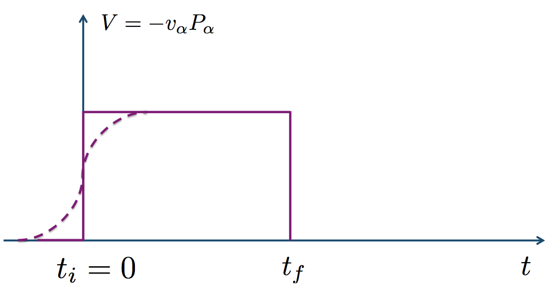
Now the results of the APT, e.g., Eq. (8), leading to the Kubo formulas in real and imaginary time are easily understood as those of the ordinary perturbation theory with respect to the velocity dependent term in the effective Hamiltonian; see Eq. (42). Indeed, if the time of the pulse is short, then we can apply an ordinary time dependent perturbation theory where the transition amplitude is proportional to the matrix element of the perturbation integrated over time, i.e.:
| (47) |
Thus, in this limit of a short pulse we simply reproduce the ordinary perturbation theory where the transition amplitude is proportional to the change of the coupling constant. Conversely, in the long time limit, the response is very different: to leading order of perturbation theory the system is excited at the initial time, then it freely evolves in a moving basis, after which it is excited again by the quench at . Thus, the transition amplitude is the sum of two terms, corresponding to the initial and final quenches. The contribution due to the initial quench comes in as a rapidly changing Rabi phase. As we discussed above, this phase averages to zero due to any dephasing mechanism, or it can be simply suppressed by a slow turning-on of the velocity. If this is the case, then we can reproduce the transition amplitudes (8) and (18) by using an ordinary static perturbation theory with respect to the perturbation for real time protocols and for imaginary time protocols.
II.6 Extracting the Berry curvature from the imaginary time dynamics. Analytic continuation of the imaginary time dynamical response to real time.
Equations (24) and (25) show that one can extract the Berry curvature as a linear response to the quench velocity in real time and the metric tensor from the imaginary time response. Real time dynamics of course corresponds to physical processes and thus can be directly realized in experiments. However, with the exception of one dimensional systems, there are very limited numerical tools which would allow for real time simulations. Imaginary-time dynamics has the advantage that it is amenable to powerful QMC as we first showed with the non-equilibrium QMC (NEQMC) approach in Ref. De Grandi et al. (2011) and later with a different quasi-adiabatic QMC (QAQMC) scheme in Ref. Liu et al. (2012). We will briefly review these approaches in Sec. IV.
Because of the opportunities offered by the NEQMC and QAQMC methods, it would be very practical to have a way to extract the Berry curvature using imaginary-time dynamics as well. This indeed becomes possible if we evolve left and right wave functions in imaginary time with different velocities, and , and evaluate the following expectation value:
| (48) |
where and are the solutions of the imaginary time Schrödinger equation for the two protocols characterized by different velocities. It is important that both and are evaluated at the same point in the parameter space. Then it is easy to see that in the linear order in the velocities and we have:
| (49) |
In particular, if , i.e. if the left wave functions is the instantaneous ground state, then the equation above is equivalent to the real time linear response (24). Very similar results apply to real-time simulations, i.e., if we compute in a real-time protocol we will get the linear response proportional to the real part of the metric tensor.
The result (49) opens the possibility of extracting the Berry curvature from numerical simulations in imaginary time. Note that the Berry curvature is non-zero only if the time reversal symmetry is broken, and, hence, the wave function is complex. In these situations QMC simulations usually suffer from the sign problem. However, it is important to mention that the time reversal symmetry can be broken by the parameter , which does not enter the time evolution and only appears in the definition of the observable we measure. In these situations, the wave function always remains real and the sign problem may be avoidable.
In imaginary time dynamics left and right states corresponding to opposite velocities naturally occur for the asymmetric expectation values. For a closely related QAQMC algorithm this issue was discussed in detail in Ref. Liu et al. (2012). Let us define the protocol where the coupling changes in imaginary time in the symmetric fashion in the interval: : . Then denoting the imaginary time evolution operator
| (50) |
we can write a generally asymmetric value of arbitrary observable as
| (51) |
where is the initial state and . Such expectation values are very straightforward to evaluate for any in e.g. Monte-Carlo simulations (see also discussion below following Eq. (76)). It is easy to see that in the middle point of the evolution this expectation value becomes equivalent to the result of the imaginary time dynamics discussed in the previous sections. Away from the symmetric point the left and right states effectively evolve with the opposite velocities so the expectation value above effectively becomes
| (52) |
As it is discussed in Ref. Liu et al. (2012) the interval around where the crossover between symmetric and asymmetric asymptotics happens vanishes as .
From the analytic properties of the wave-function discussed below Eq. (20) it is clear that the real time expectation value of the observable can be obtained by the analytic continuation of Eq. (52) to the imaginary velocity . Indeed as we noted earlier to get the real time result for the wave function and its complex conjugate one needs to analytically continue the velocity to the imaginary axis in the opposite ways . However, because in Eq. (52) and are evaluated at opposite velocities both have to be analytically continued in the same way . As a result the analytic continuation works for the observable . It is interesting that formally this analytic continuation is valid perturbatively to all orders in . In particular, this implies that the leading asymptotic of off-diagonal observables in the asymmetric points in (51) will be given by the Berry curvature multiplied by the velocity and for the diagonal observables the leading asymptotic will be quadratic in velocity but will have a negative sign (i.e. opposite in sign to the real time asymptotic).
II.7 Extension to non-linear quench protocols
The linear response analysis carried out above was based on the assumption that near the point of measurement the quench velocity is non-zero. This is the case for generic protocols. However, it is also possible to especially design protocols where one approaches the point of measurement with some other power law characterized by the exponent (see also Ref. De Grandi et al., 2010):
| (53) |
Here the parameter:
| (54) |
is the adiabaticity parameter, which plays the role of the quench amplitude for sudden quenches (), quench velocity for linear quenches (), quench acceleration for quadratic quenches (), and so on. We should note that, with the definition (53) for a linear quench, is actually a negative velocity. However, the convention above is more natural for non-linear protocols, in particular for noninteger values of . In Ref. Chandran et al. (2012) it was also analyzed the case when is negative and were found different behaviors. In this work we will not be concerned with such situations.
To evaluate the leading non-adiabatic response for quenches according to (53) with arbitrary we need to perform the asymptotic analysis of Eqs. (4) and (16) using Eq. (53) for the dependence of and taking the asymptotic limit . In this limit the matrix elements and the energy spectrum entering Eqs. (4) and (16) are approximately constant. Then, as an example, in imaginary time Eq. (16) reduces to:
| (55) |
where the matrix element and the energy difference are computed at the point of measurement: . The integral is taken along the actual path and is readily evaluated in the long-time limit:
| (56) |
For the linear quench this expression reduces to the leading term in Eq (18), keeping in mind that for we have ; see Eq. (53). Similarly, in real time we find
| (57) |
Using these excitation amplitudes we can easily find linear response expressions for the generalized forces extending Eqs. (24) and (25).
In real time:
| (58) |
while in imaginary time:
| (59) |
Here we have defined:
| (60) | |||||
As for the linear quenches the difference between real and imaginary time transition amplitudes is contained in the phase factors. One can always eliminate these factors artificially by considering separately left and right states, e.g., in the imaginary time evolution and forming the appropriate linear combinations similarly to Sec. II.6. For diagonal observables such as the energy or generic observables which are measured not instantaneously after the quench at but after allowing the system to relax to the diagonal ensemble, the phases in Eqs. (58) and (59) do not matter. Thus, to leading order in the responses in real and imaginary time coincide and are given by:
| (61) |
where:
| (62) |
This expression opens a way of measuring the symmetric part of the geometric tensor in real-time experiments. For example, one could measure the excess heat: for a protocol with . In this case reduces to the metric tensor .
III Universal scaling near quantum critical points
The linear response theory presented above allows one to associate deviations from adiabaticity of various observables through different susceptibilities. These susceptibilities are in turn expressed through integrals of non-equal time correlation functions and, in particular, are very sensitive to their long time asymptotics. However, in gapless regimes, specifically, near continuous phase transitions, these susceptibilities may diverge and the linear response theory then breaks down. In these situations one can extend standard scaling theory of continuous phase transitions to non-equilibrium setups.
The scaling hypothesis originally introduced by Pokrovsky-Patashinsky and Kadanoff (see, e.g., Refs. [Zinn-Justin, 2002; Sachdev, 1999] for references) is based on the conjecture that universal physics near continuous phase transitions depends on the microscopic parameters only through the correlation length. For quantum phase transitions, which are relevant for our work here, the correlation length universally diverges with the tuning parameter Sachdev (1999) as:
| (63) |
where is the correlation length exponent. For a multi-dimensional parameter space one can have different exponents along different directions. In this case there is more than one correlation length. Then, in finite size systems the scaling hypothesis states that the expectation value of any observable can be written in the following scaling form:
| (64) |
where the first constant term represents a non-universal non-critical contribution to , while is a universal number which defines the scaling dimension of the operator , is the system size and is a universal function. Various two-point correlation functions can be represented in a similar form Sachdev (1999) where instead of the system size we use the separation between points. By definition the scaling dimension of the tuning parameter is .
In general, the scaling dimensions of the coupling and the corresponding generalized force are independent. But there is an important exception, namely, when the coupling is relevant, i.e, this coupling drives the system to or away from the critical point. Then the scaling dimension of the product must be equal to , the scaling dimension of the energy, and thus we must have . If we are dealing with marginal perturbations which keep the system in the gapless regime, e.g. which lead to renormalization of the velocity, then we generally have to set (corresponding to scaling dimension of equal to zero) leading to . In this work we will assume that the driving term in the Hamiltonian is either relevant or marginal but that the observable has an arbitrary scaling dimension . The generalization to situations where the driving term is irrelevant is straightforward.
As it was argued in Refs. [S. Deng, 2008; De Grandi et al., 2010; De Grandi et al., 2011; Kolodrubetz et al., 2011, 2012; Chandran et al., 2012; Liu et al., 2012] the scaling ansatz (64) can be extended to non-equilibrium situations if we add the quench velocity as another scaling variable. In particular, since we can expect that the scaling dimension of the velocity is . This scaling dimension implies that there should be another length scale associated with the velocity :
| (65) |
For generic power law protocols characterized by the exponent [see Eq. (53)] the above result immediately generalizes to:
This length scale is indeed the Kibble-Zurek length, which was first introduced by Zurek Zurek (1985) for classical phase transitions in relation to the Kibble-Zurek mechanism Kibble (1976); Zurek (1985) and later reintroduced in Refs. [Polkovnikov, 2005; Zurek et al., 2005] for quantum phase transitions. Physically describes the length scale beyond which the system effectively freezes and cannot follow the instantaneous ground state. For multicritical points with more than one direction corresponding to different critical exponents, can depend on the direction of the quench Mukherjee et al. (2011). Now one can use this additional length scale to extend the ansatz for both real and imaginary time evolution (64) to:
| (66) |
Here and describe the coupling and its rate of change at the point where we perform the measurement of our observable .
The asymptotics of the scaling function can be often determined from qualitative considerations. Thus, if , then the system effectively behaves adiabatically and we should recover the scaling behavior pertaining to the static equilibrium. In the opposite limit, depending on the ratio of and , we should recover a similar crossover between the linear response discussed earlier and non-equilibrium universal scaling. For we have if there is a non-vanishing relevant component of the geometric tensor or in cases where we expect quadratic scaling with the velocity, e.g., if is a diagonal observable. This asymptotic predicts a non-trivial scaling of the observables with the system size for very slow protocols. In the opposite limit , we expect the extensive observables to scale linearly with the system size, i.e., . While for intensive observables should saturate to a constant value independent on the system size, such that .
These simple considerations well reproduce the scaling behaviors derived earlier. For example, we expect that the density of defects is intensive and that the number of defects has scaling dimension zero (more accurately this statement applies to the log fidelity De Grandi et al. (2010)) and thus:
| (67) |
is the well known Kibble-Zurek scaling form Zurek (1985). Similarly we can recover the scaling of the excess energy density for quenches ending near a quantum-critical point: , which follows from noting that the scaling dimension of the Hamiltonian is (or, equivalently, that the scaling dimension of the Hamiltonian density is ). These scaling considerations equally apply to imaginary-time (dissipative) and real-time dynamics. The only difference is that in the low-velocity limit the response is given by different susceptibilities, which, however, have the same scaling properties. Note that while in this paper we focus on quantum-critical points, the general considerations equally apply to thermal transitions, as it was emphasized in Ref. [Chandran et al., 2012].
IV Time-evolving quantum Monte Carlo algorithms
One of the primary reasons for considering imaginary-time dynamics is that it is amenable to numerical simulation with modified QMC methods. This way, one can go beyond one dimension (where DMRG is applicable in real time) for a rather broad class of systems for which sign problems can be avoided. This class coincides with that for which equilibrium QMC methods can be applied.
Standard QMC algorithms can be classified into finite-temperature methods, where the goal is to compute a quantum-mechanical thermal average of the form:
| (68) |
and ground-state projector methods, where some operator is applied to a “trial state” , such that approaches the ground state (up to an irrelevant normalization factor) when and an expectation value (which is what normally is computed, although one can also stochastically generate the wave function)
| (69) |
approaches the true ground state expectation value, . For the projector, one can use with large or a high power of the Hamiltonian, . If in the latter case one uses with of the former approach, the same rate of convergence applies for a given system volume (which follows, e.g., from a series expansion of the exponential, which for large is dominated by powers of the order , where is the ground state energy).
The differences between and projector methods can be thought of in terms of different boundary conditions in imaginary time: The trace taken at in (68) corresponds to periodic boundaries while the projector methods correspond to opening up these boundaries and replacing them with the ones corresponding to the trial state. Completely open boundary conditions correspond to the trial state being the equal superposition of all states in the basis used.
The time-evolving QMC methods we have developed are essentially modified projector algorithms. In the original NEQMC approach the exponential operator for a fixed Hamiltonian is replaced by the Schrödinger evolution operator in imaginary time,
| (70) |
where indicates time ordering. As in equilibrium QMC schemes, there are several ways to deal with the exponential. In the context of spins and bosons, the most frequently used methods are based on (i) the Suzuki-Trotter-decomposition, which leads to world-line methods Hirsch et al. (1982), (ii) the continuous-time version of world-lines (e.g., the worm algorithm Prokofe’v et al. (1998)), and (iii) the Taylor expansion leading to the SSE method Sandvik and Kurkijärvi (1991); Sandvik (2010) (see Ref. Sandvik (1992) for a recent review of these approaches). The latter two methods are not affected by any approximations (beyond statistical sampling errors), while (i) has a discretization error.
In the NEQMC algorithm a series expansion is employed for (70) in the non-equilibrium case, while in the more recently introduced QAQMC method the power of the Hamiltonian used in standard projector methods is replaced by a product of evolving Hamiltonians. It was shown in Ref. Liu et al. (2012) that the product evolution reproduces imaginary-time Schrödinger dynamics up to the leading corrections in to the adiabatic evolution. In practice, this kind of method is easier to implement than the NEQMC scheme, and, moreover, one can obtain results for all times between the initial and final Hamiltonian in a single run. We here briefly review the two methods.
IV.1 Non-equilibrium Schrödinger approach
In the NEQMC scheme first proposed in De Grandi et al. (2011) the exponential in (70) is expanded in a power-series and applied to an initial state :
| (71) |
The Hamiltonian is a sum of terms,
| (72) |
where the index can refer to lattice sites, links, etc., and is the total number of these operators. A minus sign has been included for convenience. The operator product in (71) is then written as a sum over all strings of the operators . Truncating at some maximum power (adapted to cause no detectable error—see Sandvik (1992) for a discussion of this issue in the SSE method) and introducing a trivial unit operator , one obtains:
| (73) |
where , denotes the sum over all possible sequences of operators and is the number of indices .
At this stage a basis should be chosen. For spin systems, this would normally be the standard basis of the spin components: . If the initial state has some simple known expansion in this basis, , this can be used in (73). The scheme is particularly simple when using the equal superposition, e.g., for an system, but other states can be used as well. For models with spin-isotropic interactions, such as the Heisenberg model, it is easy to use amplitude-product states in the singlet sector Sandvik and Evertz (2010). One can also start with the ground state of some Hamiltonian , by adding to (71) a projection with that fixed Hamiltonian before the quench with the time dependent is applied.
For practical implementations of the QMC scheme, the terms of should have the property that , where is a basis state. In the standard spin basis, this implies that is either a diagonal or off-diagonal operator (i.e., denotes not only a lattice unit but also refers to either a diagonal or off-diagonal part). A string of operators and their associated time values, along with a state then constitute a configuration, and the QMC simulation amounts to importance-sampling of these configurations, which strongly resemble those of a path integral.
To guarantee the absence of a sign problem we need to place certain conditions (which are not always possible to satisfy) on the matrix elements , i.e., the product of all matrix elements corresponding to a term in (73) has to be positive. While this is a limitation of the QMC approach in general, the class of accessible models is still large and includes highly non-trivial and important systems (see Ref. Kaul et al. (2012) for a recent review of quantum spin models without sign problems).
Expectation values are computed by sampling the normalization written with (73). The procedures are very similar to those used in the standard SSE and ground-state projector methods Sandvik (1992, 2003); Sandvik and Evertz (2010). The main difference is that each operator is associated with a time value. The simplest way to deal with the times is to sample them completely independently of the operator and state updates, i.e., the latter are performed with fixed time values, according to one of the standard schemes Sandvik (1992, 2003); Sandvik and Evertz (2010), and the times are updated without changes in the operators and states. A segment of times, , can be simultaneously updated by generating numbers within the range , then order these times according to a standard scheme scaling as W. H. Press and Vetterling (2007). The ordered set is then inserted in place of the old set of times, with a Metropolis acceptance probability obtained from (73). The number can be adjusted to give an acceptance probability close to .
As discussed in Sec. II.6, in addition to conventional expectation values, it is also useful to study asymmetric expectation values defined with two different time evolution operators and , e.g., corresponding to different velocities: . This can be done with a simple generalization of the above NEQMC algorithm.
IV.2 Quasi-adiabatic approach
One may ask whether the role of the time integrals in Eq. (71) is crucial. Clearly, they are needed in order to obtain a mathematically exact expansion of the time evolution operator (70), but one can, in fact, also formulate a scheme similar to time evolution without these integrals, by acting on the initial ground state of with a product of evolving Hamiltonians:
| (74) |
where we consider the parameter changing according to
| (75) |
and is the single-step change in the tuning parameter. One can also consider a non-linear grid of points, but here we focus on the linear evolution. It is clear that approaches the ground state of the final Hamiltonian in the limit of large (up to an irrelevant normalization).
In Ref. Liu et al. (2012) it was also demonstrated, using APT, that , where is the system volume, plays the role of a velocity , and that captures the leading non-adiabatic corrections in to the imaginary-time Schrödinger evolution. This is sufficient for recovering all the dynamical susceptibilities that we discussed in this work.
Moreover, one can also consider generalized (asymmetric) expectation values of the form:
| (76) |
where only the special case corresponds to a true quantum mechanical expectation value but also the generic quantities contain useful dynamic information and obey dynamic finite-size scaling. A significant advantage of QAQMC over the NEQMC approach is then that one can compute for all simultaneously in a single simulation for operators that are diagonal in the basis used. Such a simulation amounts to generating terms (paths) contributing to the normalization and successively measuring diagonal observables after propagation of the state with operators, for on a suitable grid.
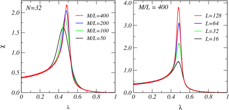
Figure 2 shows examples of results obtained with the QAQMC method in simulations of the 1D transverse-field Ising model, which we introduce in the next section. The quantity shown is the magnetization fluctuation,
| (77) |
which exhibits a peak close to the known quantum-critical point at . The peak grows both as a function of the size and , and one can subject the data to various forms of finite-size and finite-velocity scaling, examples of which are discussed in Ref. Liu et al. (2012).
As an alternative to computing expectation value based on evolving the same state from the left and the right in (76), one can also carry out QAQMC simulations as a one-way evolution. In the simplest case, the left state is the ground state of and the right state is the ground state of . The single sequence (74) between these state will then smoothly connect them, and, again, this evolution captures the leading non-adiabatic corrections in to the standard Schrödinger dynamics, with . As we discussed earlier (see Sec. II.6) asymmetric expectation values including one way evolution can be used for computing the Berry curvature in the system.
V Transverse field Ising model in one dimension
We now investigate the results of the previous sections by analyzing quenches in real or imaginary time of the one-dimensional (1D) transverse field Ising model. This model maps onto free fermions and, thus, it is easily solvable. It was used to rigorously demonstrate the universal scaling relations both for equilibrium phase transitions Sachdev (1999) and various aspects of quantum dynamics, including the Kibble-Zurek scaling Dziarmaga (2005). Furthermore, using a closely related model it was recently demonstrated that the universality of slow quantum dynamics does not rely on integrability Kolodrubetz et al. (2012). We also point out that this model was extensively used to study the dynamics following sudden quenches (see e.g. Refs. McCoy et al. (1971); Calabrese et al. (2011); Iglói and Rieger (2011); Schuricht and Essler (2012)). Here we will use this model again for the purpose of a detailed comparisons between real and imaginary time dynamics, to establish that the universal aspects are identical. We will also demonstrate how one can use this universality to accurately extract the equilibrium transition point and the critical exponents using non-equilibrium protocols.
The 1D transverse-field Ising model is defined by the Hamiltonian:
| (78) |
where and are Pauli matrices and are nearest neighbours sites. The parameters and control the nature of the quantum state: for the system is a quantum paramagnet, while for it is in a magnetically ordered phase. The point of this spin chain is a quantum critical point (QCP) separating the two different phases.
V.1 Imaginary time quench of the transverse field Ising model: exact solution
We investigate the dynamical response of the system in the vicinity of the QCP by changing in time either or . Quenches in real time of the Ising model have been considered previously De Grandi and Polkovnikov (2010), while less is known in imaginary time. In Ref. [De Grandi et al., 2011] we have fixed and considered a particular quench protocol for : , starting in the ground state at and ending at the QCP at . We can implement a similar process fixing and changing as . If instead we change as , then we approach the QCP from the initially ordered (ferromagnetic) phase. All these protocols give a very similar scaling behavior of the observables. Thus, for extracting analytical results we will focus on the particular protocol:
| (79) |
In the next section we will illustrate our results with numerical simulations, in which we also consider different protocols.
V.1.1 Spectrum of the Ising chain
It is well known that the Hamiltonian (78) can be mapped to that one of non-interacting fermions using the Jordan-Wigner transformation Sachdev (1999); Dziarmaga (2005). Because of translational invariance, the relevant excited states are only those which contain pairs of quasi-particles with opposite momenta. As a result, in this reduced Hilbert space the Hamiltonian of the system splits into a direct sum of Hamiltonians describing two-level systems with the states: and corresponding to empty and filled fermionic levels with momenta , respectively:
| (80) |
where:
| (81) |
Each of these Hamiltonians has the following eigenvectors:
| (82) |
where:
| (83) |
corresponding to the eigenenergies with . It is easy to check that:
| (84) |
where we have used .
V.1.2 Linearized spectrum: exact solution
In the adiabatic limit, where only low momentum modes contribute to the excitations, we work with the linearized spectrum of the Ising model. Then the Hamiltonian (81) simplifies to and Eqs. (85) and (86) reduce to:
| (89) | |||
| (90) |
These equations can be solved exactly analytically (we point out that this problem is the imaginary-time counterpart of the half Landau Zener (LZ) problem analyzed in Refs. Vitanov, 1999; Damski and Zurek, 2006; De Grandi and Polkovnikov, 2010). It is convenient to rescale the variables, , , and differentiate both of these equations with respect to time. We then obtain and . Each of these equations is of the type , which has two generic solutions: and , where is the confluent hypergeometric function. The generic solutions for Eqs. (89) and (90) are therefore:
| (91) |
| (92) |
The coefficients are determined by the initial conditions on the wave function at time and two auxiliary conditions, e.g., and (continuity at ). These last two equations give , , while and are set by the requirement that the system was in its ground state in the distant past: and .
Using the expansion of the hypergeometric function when :
we find that:
| (93) |
The resulting probability of being in the excited state at the end of the evolution for is found by overlapping the final wave function with the excited state at :
| (94) |
Therefore we have:
| (95) | |||||
where we point out that, since for any and , we have and . Restoring the dependence on using the substitution we obtain:
| (96) |
| Observable | |||
|---|---|---|---|
| Exact sol. and APT | Exact sol. | APT | |
V.2 Observables
In the following we present some observables that describe the response of the system to the quench in Eq. (79). Their scaling behavior is derived from the exact solution using the excitation probability in Eq. (96). The results are summarized in Table 1, where they are also compared with the correspondent scaling found by adiabatic perturbation theory (APT).
V.2.1 Excess energy Q
We consider the total excess energy of the system (energy above the instantaneous ground state energy):
| (97) |
The scaling predictions in Eq. (25) apply to this case when the observable is associated with the Hamiltonian operator: , according to our definition of generalized force in Eq. (22). In this case, since we are dealing with a diagonal operator, the geometric tensor is identically zero [see Eqs. (26) and (34)] and the response is quadratic and, in this case of a quench of a single parameter, is proportional to a single component (Eq. 30):
| (98) |
The response to the quench, both in real and imaginary time, is:
| (99) |
From the scaling dimension of the susceptibility it is possible to extract the scaling behavior of , as already done in Ref. [De Grandi et al., 2011], and to take into account the finiteness of the system, as discussed in Section III, without knowing the details of the model. The expected scaling behavior is stated in Table 1. By applying APT to the specific Ising Hamiltonian under investigation, we could also extract the numerical prefactors of the scaling, as we will explain in the next section.
From the exact solution presented in section V.1, we evaluate the total excess energy at the final critical point in the scaling limit as:
| (100) |
In the limit , we convert the sum into an integral to find
| (101) |
In the limit : and the total excess energy becomes:
| (102) |
where we used anti-periodic boundary conditions for fermions which map to periodic boundary conditions for spins (see Ref [Burkhardt and Guim, 1985] for details).
V.2.2 Log-fidelity
The logarithm of the fidelity , in the perturbative regime that we are considering, according to Eq. (23), can be approximated as: . Therefore the scaling of the log-fidelity can be extracted from that of the generalized force corresponding to the identity operator: , as it is easy to see from our definition in Eq. (22). Based on the same reasoning as above for the excess energy, the linear response for this observable vanishes, and the coefficient for the quadratic scaling is:
| (103) |
From the exact solution (see also Ref. Rams and Damski (2011)) we can calculate using:
| (104) |
Then in the limit , transforming the sum to an integral we immediately find , while in the opposite limit .
V.2.3 Transverse Magnetization
Finally we study the transverse (excess) magnetization
| (105) |
According to the definition in Eq. (22), corresponds to the expectation value of the observable , i.e., the generalized force with respect to the coupling constant that is quenched in time, which in our case is . Therefore, from Eq. (25) we expect the scaling:
| (106) |
where it should be noted that . We extract the value of from the exact solution a follows: we evaluate for each momentum the expectation value at the end of the process (): , and the sum over all momenta:
| (107) |
Evaluating this expression in the limit we find , while in the opposite limit .
These results from the exact solution are compared in Table 1 with the ones from APT. The agreement is very good, we will comment on this in more detail in the following section.
We point out that if instead we would perform a quench changing , with (as we did with QMC in Ref. De Grandi et al., 2011), the correspondent generalized force is now found with . It corresponds to the observable:
| (108) |
which is the excess interaction energy, or -energy. Therefore, the observables and have the same scaling behavior respectively for a quench of the coupling and of the coupling . When we deal with the QMC simulations and the numerical solution of the differential equations, it is in practice more convenient to perform a quench of the coupling, therefore in the following, when presenting the data we will use the observable .
V.3 Adiabatic perturbation theory for the transverse field Ising model
The exact solution for the quench dynamics in imaginary time of the 1D transverse-field Ising model provides a good opportunity to test the APT method presented in Sec. II. The APT analysis in this case is very accurate, agreeing very well with the exact solution, as shown in Table 1. The basic ingredient of the APT is the transition amplitude , which in terms of the tuning parameter becomes De Grandi et al. (2011):
| (109) |
For the transverse-field Ising model the lowest excitations correspond to flipping the effective spin from to (corresponding to exciting two Bogoliubov’s fermions with opposite momenta) characterized by the matrix element in Eq. (84) and the energy difference . Therefore the transition amplitude from the ground to the excited state is:
| (110) | |||||
This expression simplifies in the slow limit, where we can use the linearized spectrum:
| (111) |
Using these transition amplitudes instead of the exact expressions found in the previous section we recover the last column in Table 1.
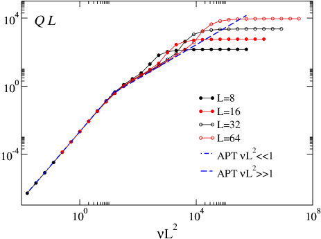
In Fig. 3 we plot the excess energy for different system sizes as a function of computed from the exact solutions of the Schrödinger equation [solving numerically Eqs. (89) and (90)]. In the same plot we also show the APT results for the infinite size. The agreement between the two methods is excellent when sufficiently large systems are used for the exact solution.
In most situations the exact solution for a time-dependent problem is not readily available. The good agreement we found here suggests that one can make many qualitative and even quantitative statements about the dynamics using the adiabatic perturbation theory, which only requires the integration of static quantities.
VI Observables in real and imaginary time quenches of the Ising model
According to the results presented in the previous sections, it follows that the imaginary-time dynamical protocols give very similar results as the real-time protocols considered earlier De Grandi and Polkovnikov (2010). This implies, in particular, that imaginary-time quantum evolution with a time evolving Hamiltonian can be used for simulations of real-time non-equilibrium dynamics, including, e.g., realizations of the quantum Kibble-Zurek mechanism Zurek et al. (2005). However, there are still also important differences between the two types of dynamics. Firstly, the imaginary-time evolution clearly breaks time-reversal symmetry and this introduces a strong asymmetry between the initial and final times of the evolution. Thus, in real-time dynamics, the system is constantly excited during the evolution and these excitations propagate in time. On the contrary, during the imaginary-time evolution the system always relaxes toward the ground state, and the effects of non-adiabaticity are visible only when approaching the final state, i.e., the critical point. For example, in real-time evolution the ground state fidelity and the diagonal entropy Polkovnikov (2011) (which are observable independent measures of non-adiabaticity) are identical for the time-reversed protocols. In particular, the degree of non-adiabaticity is the same if one considers protocols which start or end at the quantum critical point. In imaginary-time evolution this is not the case. If one passes a singularity, like a critical point, in a real-time process, then it will always result in non-analyticities in various observables (the defect density in the case of Kibble-Zurek mechanism is an example of this). In imaginary-time evolution the singularities in the observables will show up only if one ends the process at this singularity or in its close vicinity.
In this section we analyze closely the behavior of the observables in the case of quenches of the transverse-field Ising model, comparing the exact solutions for the real- and imaginary-time cases. For simplicity we consider here the protocol already analyzed in Ref. [De Grandi et al., 2011], where we fix and ramp linearly in time to end at the critical point, i.e., and , in imaginary and real time, respectively, with the final time: . Then the scalings of the excess energy, fidelity and magnetization in real and imaginary times look nearly identical. Since real-time evolution in this model was analyzed earlier in different papers Dziarmaga (2005); De Grandi and Polkovnikov (2010) we will omit the details of the calculation and only present the final results. We note that in Ref. [De Grandi and Polkovnikov, 2010] we analyzed a linear quench where one starts at the quantum critical point. Because of the symmetry of the transition probabilities with respect to time reversal the analysis applies as well to the process we are interested in here, where one ends the quench at the quantum-critical point. The only subtlety appears in the analysis of the -magnetization, which is an off-diagonal observable and which depends on the phase of the transition amplitude. We will comment on this subtlety below.
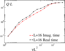
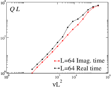
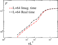
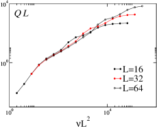
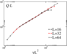
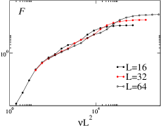
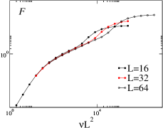
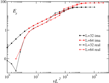
In Table 2 we present the comparison of the scaling of several observables for linear quenches to the QCP in real and imaginary time, obtained from the exact solution of the transverse-field Ising model (see Sec. V.1 for the imaginary-time case and Refs. Dziarmaga (2005); De Grandi and Polkovnikov (2010) for the real-time case). In Figures 4, 5, and 6 we plot the corresponding quantities obtained by solving numerically the Schrödinger equation. The definition of the observables was given in the previous Section V. As mentioned before, since we are quenching (and not , to be consistent with the protocol used in QMC simulation presented in following sections), the observable which gives the fidelity susceptibility in the linear response is the excess interaction energy [see Eq. (108)]. It is expected to scale in the same way as .
Overall we find very good agreement and almost identical behavior between the imaginary and the real time cases. A more careful analysis is nevertheless necessary. For the diagonal observables, the excess energy and the log-fidelity , the scaling behaviors are the same in real and imaginary time and in agreement with the APT predictions presented in the previous section. In particular, in the limit even the prefactors coincide—indeed, in this limit the analytic expression are identical. In the opposite regime the prefactors are slightly different. In this limit, the real-time dynamics presents a more oscillating behavior: see for instance the plots of the excess energy in Fig. 5. A similar behavior was also observed in Refs. Kolodrubetz et al. (2011, 2012).
The case of the excess -energy or magnetization along the -direction [as defined in Eq. (105)] requires more attention. Indeed this quantity, as mentioned before, corresponds to the generalized force with respect to the coupling that drives the dynamics. Working out the asymptotic scaling behavior from the scaling dimension in the limit of we find in both real and imaginary times, according to Eqs. (24) and (25). Concerning the limit , in imaginary time, from the exact solution [see Eq. (107)] we know that . In the real-time case, from analyzing the exact solution we can infer that the behavior for small is non analytic, decaying exponentially as . Such behavior is visible in the plot in Fig. 6; for large values of (but not too large, as finite-size effects also are apparent) the slopes of the real- and imaginary-time functions are the same, the data being shifted by a factor of according to the predictions. For the imaginary-time function decays analytically with slope as expected, while in the real-time case there is a more rapid drop reflecting the non-analyticity of the function.
| Observable | Real | Imag. | Real | Imag. |
|---|---|---|---|---|
| 0 | ||||
VII Application: detection of quantum-critical points
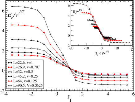
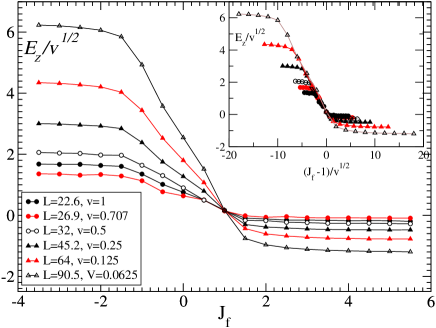
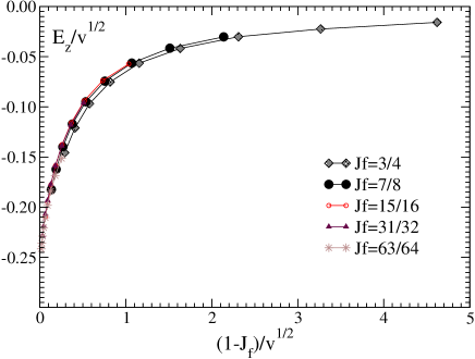
A useful application of the universal scaling presented in the previous sections can be found by considering quenches in either real or imaginary time that sweep through the QCP and end at different final amplitudes . In this case, as discussed in Sec. III, the length scale is not diverging anymore and participates in the scaling behavior along with and the system size . For a generalized force we then expect a scaling behavior as the one given in Eq. (66):
| (112) | |||||
as was already suggested in Ref. De Grandi et al. (2011). If we perform several quenches changing the final amplitude and plot for each of them the rescaled quantity , we expect all the curves (asymptotically for sufficiently large ) to cross at the location of the QCP, since when the rescaled quantity does not depend on anymore. We have performed such an analysis for an imaginary-time quench of the form , and the correspondent real-time one (replacing with ). Sweeping across the critical point, i.e., starting from a negative and ending at some positive value, and looking at the -energy as defined above in Eq. (108), we expect:
| (113) |
In Fig. 7 we show the results for imaginary- (top graph) and real-time (bottom graph) quenches based on the numerical solution of the Schrödinger equation. The expected behavior is confirmed in both cases, all the lines cross around where the QCP is located. Therefore, through this type of analysis it would be possible to locate the position in the parameter space of a QCP of a system that cannot be solved exactly and of which the position of the critical point is not known. The universal behavior described by Eq. (113) is furthermore confirmed by the collapse of the data when plotting versus the rescaled quantity : see the insets of Fig. 7. As expected, a similar collapse is also observed if we perform a quench that does not reach the QCP but ends just before it, as we show by the data in Fig. 8. These results were obtained by numerical simulation of the 1D Ising model with the NEQMC method introduced in Ref. De Grandi et al. (2011) (and discussed also above in Sec. IV), using it to perform a linear quench ending at different values of the final amplitude and approaching .
VIII Universal relaxation to equilibrium after a quench
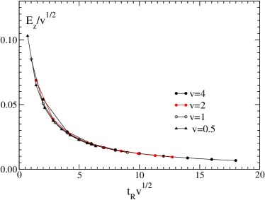
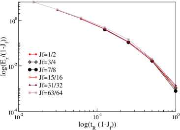
Up to this point we have been concerned with the scaling of the observables right at the end of a quench, in particular at the final time, when the Hamiltonian of the system has reached the QCP or, as in the previous section, some other amplitude . Here we want to address the scaling behavior that follows subsequent to the quench, when the system starts relaxing governed by a fixed Hamiltonian. Therefore we let the system evolve after the end of a quench with the fixed final Hamiltonian for a variable length of time, that we call , and we look at the behavior as a function of , that we call the relaxation time. Based on the scaling arguments that have lead us to Eq. (66), we argue that, if we let the system evolve after the quench for a time , then we expect [for a generic -th power quench as in Eq. (53)]:
| (114) |
This means that the relaxation time itself comes into play in the universal scaling behavior as an additional “length” scale to be compared to the other characteristic lengths of the system. For sudden quenches this conjecture was recently suggested and tested in Ref. Torre et al. (2012). If the system size is large enough, for instance, we expect the quantity to be the rescaled variable that characterize the universal relaxation after quenches with different velocities. As before, we have checked this behavior for the -component excess energy from the exact solutions [solving numerical Eqs. (89) and (90)] for a linear quench, see Fig. 9, and with NEQMC for a sudden quench see Fig. 10.
IX Summary and conclusions
We have presented an overview of general aspects of non-adiabatic response of physical observables to slowly changing parameters, both in imaginary (Euclidean) and real time. There are many similarities between the imaginary- and real-time response, which we demonstrated by calculating the leading first- and second-order non-adiabatic corrections of physical observables. We identified the corresponding susceptibilities and expressed them through the non-equal time correlation functions. In particular, we extended the traditional Kubo response theory to describe the response of systems to perturbations which are slow but can be arbitrarily large in amplitude. The components of the geometric tensor (the metric tensor and the Berry curvature) naturally emerge as response functions of physical observables to the quench velocity.
Both real- and imaginary-time dynamics near continuous phase transitions can be used to analyze universal non-adiabatic response of the system and extract static and dynamic critical exponents, using a generalized non-equilibrium scaling theory, which we also further elaborated here. Importantly, imaginary-time dynamics is amenable to powerful Monte Carlo simulation methods. We briefly reviewed two different QMC algorithms which directly implement quantum dynamics for interacting systems. They have the same range of practical applicability (avoidability of sign problems) as conventional equilibrium finite-temperature or ground-state projection methods.
We illustrated the utility of the general theoretical formalism using the particular example of the transverse-field Ising model in one dimension. Using both exact treatments (through the standard mapping to fermions) and QMC simulations, we found that imaginary- and real-time dynamical responses indeed are very similar near the critical point, for all physical observables examined. We also found excellent agreement with predictions of adiabatic perturbation theory. We illustrated how one can use the non-equilibrium finite size scaling to accurately extract the transition point and the critical exponents.
The ideas presented in this article have many potential applications, including (i) analysing universal dynamical response near quantum phase transitions with unknown dynamical exponent, e.g., in disordered systems; (ii) applying QMC methods to implement imaginary-time quantum annealing and (using the similarity of non-adiabatic response in real and imaginary times) making predictions concerning real-time quantum annealing protocols; (iii) using non-adiabatic response of physical observables to directly extract the Berry curvature and the metric tensor (including the fidelity susceptibility) either experimentally or numerically.
Acknowledgements.
We would like to thank Cheng-Wei Liu for collaboration on the QAQMC method and for generating the data presented in Fig. 2. This work was supported by the NSF under Grant No. NSF PHY11-25915 (AP and AWS). AP also acknowledges support from Grants NSF DMR-0907039 and AFOSR FA9550-10-1-0110, and from the Simons and Sloan Foundations.References
- Schollwöck (2005) U. Schollwöck, Rev. Mod. Phys. 77, 259 (2005).
- Santos and Rigol (2010) L. F. Santos and M. Rigol, Phys. Rev. E 81, 036206 (2010).
- De Grandi et al. (2011) C. De Grandi, A. Polkovnikov, and A. W. Sandvik, Phys. Rev. B 84, 224303 (2011).
- Hohenberg and Halperin (1977) P. C. Hohenberg and B. I. Halperin, Rev. Mod. Phys. 49, 435 (1977).
- Chandran et al. (2012) A. Chandran, A. Erez, S. S. Gubser, and S. L. Sondhi, Phys. Rev. B 86, 064304 (2012).
- Kardar et al. (1986) M. Kardar, G. Parisi, and Y. C. Zhang, Phys. Rev. Lett. 56, 889 (1986).
- Huse et al. (1985) D. A. Huse, C. L. Henley, and D. S. Fisher, Phys. Rev. Lett. 55, 2924 (1985).
- Kardar (1987) M. Kardar, Nucl. Phys. B 290, 582 (1987).
- S. Deng (2008) L. V. S. Deng, G. Ortiz, Europhys. Lett. 84, 67008 (2008).
- Kolodrubetz et al. (2012) M. Kolodrubetz, B. K. Clark, and D. A. Huse, Phys. Rev. Lett. 109, 015701 (2012).
- Liu et al. (2012) C.-W. Liu, A. Polkovnikov, and A. W. Sandvik, arXiv:1212.4815 (2012).
- Mahan (2000) G. D. Mahan, Many-Particle Physics (Kluwer Academic/Plenum Publishers, New York, 2000).
- Rigolin et al. (2008) G. Rigolin, G. Ortiz, and V. H. Ponce, Phys. Rev. A 78, 052508 (2008).
- De Grandi and Polkovnikov (2010) C. De Grandi and A. Polkovnikov, Lect. Notes in Phys. 802, 75 (2010).
- Polkovnikov and Gritsev (2008) A. Polkovnikov and V. Gritsev, Nat. Phys. 4, 477 (2008).
- Gritsev and Polkovnikov (2012) V. Gritsev and A. Polkovnikov, PNAS 109, 6457 (2012).
- Avron et al. (2011) J. E. Avron, M. Fraas, G. M. Graf, and O. Kenneth, New J. Phys. 13, 053042 (2011).
- Provost and Vallee (1980) J. Provost and G. Vallee, Communications in Mathematical Physics 76, 289 (1980).
- Berry (1984) M. Berry, Proc. Royal Soc. London A 392, 45 (1984).
- Venuti and Zanardi (2007) L. C. Venuti and P. Zanardi, Phys. Rev. Lett. 99, 095701 (2007).
- De Grandi et al. (2010) C. De Grandi, V. Gritsev, and A. Polkovnikov, Phys. Rev. B 81, 012303 (2010).
- Zinn-Justin (2002) J. Zinn-Justin, Quantum Field Theory and Critical Phenomena (Oxford University Press, 2002).
- Sachdev (1999) S. Sachdev, Quantum Phase Transitions (Cambridge University Press, 1999).
- Kolodrubetz et al. (2011) M. Kolodrubetz, D. Pekker, B. K. Clark, and K. Sengupta, arXiv:1106.4031 (2011).
- Zurek (1985) W. H. Zurek, Nature 317, 505 (1985).
- Kibble (1976) T. Kibble, J Phys. A: Math. Gen. 9, 1387 (1976).
- Polkovnikov (2005) A. Polkovnikov, Phys. Rev. B 72, 161201(R) (2005).
- Zurek et al. (2005) W. H. Zurek, U. Dorner, and P. Zoller, Phys. Rev. Lett. 95, 105701 (2005).
- Mukherjee et al. (2011) V. Mukherjee, A. Polkovnikov, and A. Dutta, Phys. Rev. B 83, 075118 (2011).
- Hirsch et al. (1982) J. E. Hirsch, R. L. Sugar, D. J. Scalapino, and R. Blankenbecler, Phys. Rev. B 26, 5033 (1982).
- Prokofe’v et al. (1998) N. V. Prokofe’v, B. V. Svistunov, and I. S. Tupitsyn, JETP 87, 311 (1998).
- Sandvik and Kurkijärvi (1991) A. W. Sandvik and J. Kurkijärvi, Phys. Rev. B 43, 5950 (1991).
- Sandvik (2010) A. W. Sandvik, AIP Conf. Proc. 1297, 135 (2010).
- Sandvik (1992) A. W. Sandvik, J. Phys. A 25, 3667 (1992).
- Sandvik and Evertz (2010) A. W. Sandvik and H. G. Evertz, Phys. Rev. B 82, 024407 (2010).
- Kaul et al. (2012) R. K. Kaul, R. G. Melko, and A. W. Sandvik, arXiv:1204.5405 (2012).
- Sandvik (2003) A. W. Sandvik, Phys. Rev. E 68, 056701 (2003).
- W. H. Press and Vetterling (2007) S. A. T. W. H. Press, B. P. Flannery and W. T. Vetterling, Numerical Recipes: The Art of Scientific Computing (Cambridge University Press, 2007).
- Dziarmaga (2005) J. Dziarmaga, Phys. Rev. Lett. 95, 245701 (2005).
- McCoy et al. (1971) B. M. McCoy, E. Barouch, and D. B. Abraham, Phys. Rev. A 4, 2331 (1971).
- Calabrese et al. (2011) P. Calabrese, F. H. L. Essler, and M. Fagotti, Phys. Rev. Lett. 106, 227203 (2011).
- Iglói and Rieger (2011) F. Iglói and H. Rieger, Phys. Rev. Lett. 106, 035701 (2011).
- Schuricht and Essler (2012) D. Schuricht and F. H. L. Essler, arXiv:1203.5080 (2012).
- Vitanov (1999) N. V. Vitanov, Phys. Rev. A 59, 988 (1999).
- Damski and Zurek (2006) B. Damski and W. H. Zurek, Phys. Rev. A 73, 063405 (2006).
- Burkhardt and Guim (1985) T. W. Burkhardt and I. Guim, Journal of Physics A: Mathematical and General 18, L33 (1985).
- Rams and Damski (2011) M. M. Rams and B. Damski, Phys. Rev. Lett. 106, 055701 (2011).
- Polkovnikov (2011) A. Polkovnikov, Annals of Physics 326, 486 (2011).
- Torre et al. (2012) E. G. D. Torre, E. Demler, and A. Polkovnikov, arXiv:1211.5145 (2012).