On transition rates in surface hopping

Abstract

Trajectory surface hopping (TSH) is one of the most widely used quantum-classical algorithms for nonadiabatic molecular dynamics. Despite its empirical effectiveness and popularity, a rigorous derivation of TSH as the classical limit of a combined quantum electron-nuclear dynamics is still missing. In this work we aim to elucidate the theoretical basis for the widely used hopping rules. Naturally, we concentrate thereby on the formal aspects of the TSH.

Using a Gaussian wave packet limit, we derive the transition rates governing the hopping process at a simple avoided level crossing. In this derivation, which gives insight into the physics underlying the hopping process, some essential features of the standard TSH algorithm are retrieved, namely i) non-zero electronic transition rate (“hopping probability”) at avoided crossings; ii) rescaling of the nuclear velocities to conserve total energy; iii) electronic transition rates linear in the nonadiabatic coupling vectors. The well-known Landau-Zener model is then used for illustration.

I Introduction

Practical molecular modeling is based on the Born-Oppenheimer approximation (BOA), which allows one to decouple the fast electronic motion from the usually slower nuclear motion by introducing i) the (adiabatic) potential energy surfaces (PESs), provided by the electrons in a specific eigenstate, and ii) the nonadiabatic couplings (NACs).Born and Huang (2000) When the latter are neglected, nuclei move on a single PES. Despite the success of the BOA, there are many physical situations, such as photo-reaction, electron transfer, or any form of non-radiative electronic relaxation, which involve more than one PES.Wodtke, Tully, and Auerbach (2004) In these cases one has to take into account the coupling between various PESs.

One of the most widely applied techniques to treat nonadiabatic effects in molecular dynamics is the trajectory surface hopping (TSH), with its several variants.Tully and Preston (1971); Tully (1990); Hammes-Schiffer and Tully (1994); Webster et al. (1994); Tully (1998); Prezhdo and Rossky (1997a); Wong and Rossky (2002a, b); Bedard-Hearn, Larsen, and Schwartz (2005); Subotnik and Shenvi (2011); Subotnik (2011); Shenvi, Subotnik, and Yang (2011) The main idea behind this technique is that, while the electronic wave function is propagated coherently, the force field felt by the nuclei varies in a discontinuous, stochastic way — the nuclei move along a single adiabatic PES, selected according to the electronic population of the corresponding state; time changes in the electronic populations can result in a sudden hop to another adiabatic energy surface. In order to conserve the total energy after each hop, the nuclear velocities are rescaled. This leads to a discontinuity in the nuclear velocities which, however, is generally small since the hops are more likely to occur between PESs which are close in energy. Yet, energy conservation is obtained in a rather ad hoc way and, although it is common practice to rescale the velocities along the direction of the nonadiabatic coupling vectors (which couple different adiabatic states),Tully (1990); Hack and Truhlar (2000) in principle other choices are possible.Hack and Truhlar (2000); Bedard-Hearn, Larsen, and Schwartz (2005); Subotnik and Shenvi (2011) As a consequence, most surface hopping algorithms are justified on an empirical basis, by direct comparison with exact analytical results in model systems or experimental data. A further issue concerns the loss of electron-nuclear coherence in the course of the dynamics. This aspect is directly related to the scaling of the transition probability with respect to the nonadiabatic couplings. It is traditionally linear in standard TSH,Tully (1990) but it was recently shown to be incorrect for some model cases,Subotnik and Shenvi (2011) the effect being directly traced back to the treatment of decoherence over time.

In this work emphasis is put on the formal analysis in order to provide a basis for better understanding surface hopping techniques, rather than concentrating on numerical aspects. This aim is similar in spirit to that of previous works, Herman (1984, 1995); Wu and Herman (2006); Tully (1998) but in a simpler framework. The paper is organized as follows. In Sec. II we briefly introduce the formalism which will be used in the rest of the paper. In Sec. III we derive the equations governing the electronic transition rates at an avoided crossing by using a Gaussian wave packet limit for the nuclear wave function. The equations directly display the physics behind the TSH, i.e., the physics governing a hop at an avoided crossing followed by rescaling of the nuclear velocities in order to conserve total energy. We find that the physical source of the velocity rescaling is related to the speed of variation of the NACs and that the rescaling only affects the nuclear velocity components parallel to the NAC vectors. We further discuss some general consequences of our theoretical approach and its relevance in the context of practical nonadiabatic molecular dynamics. In Sec IV the electronic transition rates are explored by using the Landau-Zener model as a paradigmatic test case. We finally draw our conclusions and future perspectives.

II Basics

We consider a quantum mechanical system of $n$ electrons and $N$ nuclei with the total Hamiltonian $\hat{H}=\hat{T}+\hat{H}^{\mathrm{el}}$ being the sum of the kinetic energy of the nuclei, $\hat{T}=-{{\mathbf{\nabla}}^{2}_{\mathbf{R}}}/{2M}$, and the electronic Hamiltonian, $\hat{H}^{\mathrm{el}}$, which contains the kinetic energy of the electrons, the electron-electron potential, the electron-nuclear coupling, and the nucleus-nucleus potential. To keep notations simple, throughout this paper we denote the set of electronic coordinates by $\mathbf{r}$ and the nuclear ones by $\mathbf{R}$; moreover we consider all nuclei having the same mass $M$ and we use atomic units.

The nuclei are much heavier than the electrons and thus it is a natural first approximation to consider them as classical particles, having at all times well defined positions $\mathbf{R}$ and momenta $\mathbf{P}$. This suggests an adiabatic procedure where the electronic problem is solved for nuclei momentarily clamped to fixed positions in space: $\hat{H}^{\mathrm{el}}(\mathbf{R})\phi_{i}(\mathbf{r};\mathbf{R})=E_{i}(\mathbf{R})\phi_{i}(\mathbf{r};\mathbf{R})$. The (adiabatic) electronic eigenfunctions $\{\phi_{i}(\mathbf{r};\mathbf{R})\}$ depend parametrically on the atomic positions and form a complete and orthonormal set. They can be used as a basis to expand the total wave function of the system as

$$\Xi(\mathbf{r},\mathbf{R};t)=\sum_{j}\chi_{j}(\mathbf{R};t)\phi_{j}(\mathbf{r};\mathbf{R}),$$ (1)

and solve the time-dependent Schrödinger equation

$${\mathrm{i}}\partial_{t}\Xi(\mathbf{r},\mathbf{R};t)=\hat{H}\Xi(\mathbf{r},\mathbf{R};t).$$ (2)

The expansion coefficients $\chi_{j}(\mathbf{R};t)$, which depend on the nuclear positions, will be identified as nuclear wave packets. Such wave packets are neither orthogonal nor normalized. In fact, the integral $\int{\mathrm{d}}^{3N}\mathbf{R}\,|\chi_{j}(\mathbf{R};t)|^{2}=||\chi_{j}(t)||^{2}$ gives the instantaneous electronic population of the $j^{th}$ quantum state. By inserting expansion (1) for the total wave function into the Schrödinger equation (2) and projecting out the resulting equation on the electronic state $\phi_{i}$, one obtains

$${\mathrm{i}}\frac{\partial}{\partial t}\chi_{i}(\mathbf{R};t) = \left[\hat{T}+E_{i}(\mathbf{R})\right]\chi_{i}(\mathbf{R};t)$$ (3)

$$-{\mathrm{i}}\sum_{j}\mathbf{D}_{ij}(\mathbf{R})\cdot\hat{\mathbf{P}}\chi_{j}(\mathbf{R};t).$$

with

$$\mathbf{D}_{ij}(\mathbf{R})=\frac{1}{M}\langle\phi_{i}(\mathbf{r};\mathbf{R})|\nabla_{\mathbf{R}}|\phi_{j}(\mathbf{r};\mathbf{R})\rangle$$ (4)

being the NAC vectors and $\hat{\mathbf{P}}=-{\mathrm{i}}\nabla_{\mathbf{R}}$ the momentum operator for the nuclei, and where we used the notation $\langle\phi_{i}(\mathbf{r};\mathbf{R})|\hat{O}|\phi_{j}(\mathbf{r};\mathbf{R})\rangle=\int{\mathrm{d}}^{3n}\mathbf{r}\,\phi^{*}_{i}(\mathbf{r};\mathbf{R})\hat{O}\phi_{j}(\mathbf{r};\mathbf{R})$, with $\hat{O}$ a generic operator. Note that in (3) we neglected the terms $\langle\phi_{i}(\mathbf{r};\mathbf{R})|\hat{T}|\phi_{j}(\mathbf{r};\mathbf{R})\rangle$, being of the order $1/M$ smaller than the kinetic energy of the electrons.Schwabl (2007)

The NAC vectors $\mathbf{D}_{ij}(\mathbf{R})$ couple different adiabatic energy surfaces. Generally the coupling terms in Eq. (3) are of order $1/\sqrt{M}$ smaller than the electronic energy,Schwabl (2007) and therefore they can be safely neglected. In this case the adiabatic nuclear wave functions are evolved independently, i.e., their normalizations — which give the adiabatic populations — are constants of motion. The Born-Oppenheimer approximation is based on this decoupling. However, as the gap between two PESs narrows, the NAC vectors become large, as it can be seen from the following expression:Worth and Cederbaum (2004)

$$\mathbf{D}_{ij}(\mathbf{R})=-\frac{1}{M}\frac{\langle\phi_{i}(\mathbf{r};\mathbf{R})|(\nabla_{\mathbf{R}}\hat{H}^{\mathrm{el}})|\phi_{j}(\mathbf{r};\mathbf{R})\rangle}{E_{i}(\mathbf{R})-E_{j}(\mathbf{R})}\;,$$ (5)

where $E_{i}(\mathbf{R})-E_{j}(\mathbf{R})\neq 0$ and the numerator remains finite. This allows mixing between eigenstates for large enough nuclear velocities. TSH then provides a convenient approximation of the nonadiabatic molecular dynamics, i.e., of the electronic transitions that can occur along with the nuclear motion.

III Beyond the Born-Oppenheimer approximation

III.1 Time-dependent perturbation theory

A statistical reduction of a correlated electron-nuclear dynamics into occasional, independent, PES hopping is possible only if one transition (hop) is fully completed before the next can take place. This requires that the nonadiabatic coupling terms $\mathbf{D}_{ij}(\mathbf{R})$, although not negligible, are small enough to be considered as a perturbation during a short time interval $\Delta t$, as typically assumed in analogous analyses, see, e.g., Refs. Herman, 1995, 2001; Pechukas and Davis, 1972. In such a case, we can separate the Hamiltonian of the system in an unperturbed part $\hat{H}_{{0,i}}=\hat{T}+E_{i}(\mathbf{R})$ and a perturbation part $-{\mathrm{i}}\sum_{j}\mathbf{D}_{ij}(\mathbf{R})\cdot\hat{\mathbf{P}}$. The aim is to find an approximate solution of the time-dependent Schrödinger equation (3) according to the time-dependent perturbation theory. In order to achieve this aim, it is convenient to work in the interaction picture Fetter and Walecka (2003), where

$$\chi_{{i,I}} = e^{{\mathrm{i}}\hat{H}_{{0,i}}t}\chi_{{i}}\quad,$$

$${\mathrm{i}}\partial_{t}\chi_{i,I} = \sum_{j}\hat{W}_{ij,I}\chi_{j,I}\quad,$$

$$\hat{W}_{ij,I} = -{\mathrm{i}}\,e^{{\mathrm{i}}\hat{H}_{0,i}t}\left[\mathbf{D}_{ij}(\mathbf{R})\cdot\hat{\mathbf{P}}\right]e^{-{\mathrm{i}}\hat{H}_{0,j}t}\quad.$$

Note that in the adiabatic representation no time-ordering is needed in the definition of $\hat{W}_{ij}$. Therefore the solution of the equation of motion for $\chi_{i,I}$, between initial time zero and final time $t$, at first order in the perturbation $\sum_{j}\hat{W}_{ij,I}$ reads

$$\chi_{i,I}(\mathbf{R};t) \approx \chi_{i}(\mathbf{R};0)$$ (6)

$$-\sum_{j}\int_{0}^{t}{\mathrm{d}}t^{\prime}\,e^{{\mathrm{i}}\hat{H}_{0,i}t^{\prime}}\mathbf{D}_{ij}(\mathbf{R})\cdot\hat{\mathbf{P}}\,e^{-{\mathrm{i}}\hat{H}_{0,j}t^{\prime}}\chi_{j}(\mathbf{R};0).$$

III.2 Approximations through Gaussians

Eventually, ionic motion is treated classically while the computation of a hopping probability has to proceed in a quantum mechanical framework. In order to establish the link between these two descriptions, we need a semi-classical approximation for the wave functions $\chi$. Inspired by Heller’s work,Heller (1981) the initial state $\chi_{j}(\mathbf{R};0)$ is represented in terms of Gaussian wave packets

$$\mathcal{G}_{\mathbf{R}_{i}\mathbf{P}_{i}\lambda_{i}}(\mathbf{R})=\left(\frac{\lambda_{i}}{\pi}\right)^{3N/4}\exp\left[{\mathrm{i}}\mathbf{P}_{i}\cdot\mathbf{R}-\frac{\lambda_{i}}{2}(\mathbf{R}-\mathbf{R}_{i})^{2}\right]\quad,$$ (7)

as

$$\chi_{j}(\mathbf{R};0)=\alpha_{j}\mathcal{G}_{\mathbf{R}_{j0}\mathbf{P}_{j0}\lambda_{j}}(\mathbf{R}),$$ (8)

with $\mathbf{R}_{j0}$, $\mathbf{P}_{j0}$, and $\alpha_{j}$ being the average positions, average momenta, and amplitudes, respectively, of the wave packet at $t=0$ (see Appendix A for more details on the Gaussian wave packets). All Gaussians are normalized to one. The (complex) coefficient $\alpha_{j}$ regulates the contribution from each Gaussian to the whole state. It expresses the correlations accumulated in previous time steps. The propagator $e^{-{\mathrm{i}}\hat{H}_{0,j}t^{\prime}}$ in (6) then evolves this wave packet from the initial time $t=0$ to a time $t^{\prime}$. At this point we make use of a semi-classical approximation for the nuclei: in the spirit of the frozen Gaussian approximation proposed by Heller,Heller (1981) we impose that, for a short time interval, the width of the Gaussian is fixed (“frozen”) and that the time evolution of the parameters $\mathbf{R}_{j}(t)$ and $\mathbf{P}_{j}(t)$ is given by the solution of the classical equations of motion for an effective nuclear potential given by the $j^{th}$ PES. Note that the use of frozen Gaussians is a common practice both in numerical applications and formal developments in the field.Schwartz et al. (1996); Neria and Nitzan (1993); Subotnik and Shenvi (2011); Prezhdo and Rossky (1997b); Herman and Kluk (1984); Herman (2001); Herman, Akramine, and Moody (2004); Wu and Herman (2006) One can then use the following approximation:

$$e^{-{\mathrm{i}}\hat{H}_{0,j}t^{\prime}}\mathcal{G}_{\mathbf{R}_{j0}\mathbf{P}_{j0}\lambda_{j}} \approx e^{-{\mathrm{i}}(E_{j}+T_{j})t^{\prime}}\mathcal{G}_{\mathbf{R}_{j}(t^{\prime})\mathbf{P}_{j}(t^{\prime})\lambda_{j}},$$ (9)

with $T_{j}=\frac{\mathbf{P}_{j}^{2}}{2M}$, $E_{j}=E_{j}(\mathbf{R}_{j})$, and their sum $T_{j}+E_{j}$ being constant along the classical evolution. In doing so, we are neglecting the term $-\int_{0}^{t^{\prime}}{\mathrm{d}}t\,\dot{\mathbf{P}}_{j}(t)\cdot\mathbf{R}_{j}(t)$ in the quantum phase accumulated during the time evolution. This approximation is justified for small momentum changes during short-time propagation, which is in line with our derivation. In the following, we will refer to this semi-classical limit as the wave packet limit. Note that this limit is in the spirit of the short-time expansion to a semi-classical golden rule employed, e.g., in Refs. Neria and Nitzan, 1993; Schwartz et al., 1996; Prezhdo and Rossky, 1997b, 1998.

For the sake of simplicity, we use a multivariate Gaussian with the same (frozen) width $\lambda_{j}$ for all nuclear Cartesian coordinates. This is justified in the classical limit $\lambda_{j}\rightarrow\infty$, which will be taken at the end of our derivation. Moreover in the following we will drop the time dependence of the average positions and momenta, if not needed. At each time the Gaussian wave packets fulfill the completeness relation

$$\delta^{3N}(\mathbf{R}-\mathbf{R}^{\prime})=\int{\mathrm{d}}^{3N}\mathbf{P}_{k}\int{\mathrm{d}}^{3N}\mathbf{P}_{\ell}\mathcal{G}_{\mathbf{R}_{i}\mathbf{P}_{k}\lambda_{i}}(\mathbf{R})\,\mathcal{I}_{\mathbf{R}_{i}\lambda_{i}}^{-1}(\mathbf{P}_{k},\mathbf{P}_{\ell})\mathcal{G}^{*}_{\mathbf{R}_{i}\mathbf{P}_{\ell}\lambda_{i}}(\mathbf{R^{\prime}}),$$ (10)

where $\mathcal{I}_{\mathbf{R}_{i}\lambda_{i}}^{-1}$ is the inverse of the overlap $\mathcal{I}_{\mathbf{R}_{i}\lambda_{i}}(\mathbf{P}_{k},\mathbf{P}_{\ell})=\langle\mathcal{G}_{\mathbf{R}_{i}\mathbf{P}_{k}\lambda_{i}}|\mathcal{G}_{\mathbf{R}_{i}\mathbf{P}_{\ell}\lambda_{i}}\rangle$ (see Appendix A for details). Inserting (8) and (10) in (6) and applying the wave packet limit (9) yields

$$\chi_{i,I}(\mathbf{R};t) \approx \chi_{i}(\mathbf{R};0)-\sum_{j}\alpha_{j}\int_{0}^{t}{\mathrm{d}}t^{\prime}\int{\mathrm{d}}^{3N}\mathbf{P}_{k}\int{\mathrm{d}}^{3N}\mathbf{P}_{\ell}\,$$ (11)

$$\qquad e^{{\mathrm{i}}({E_{i}}+T_{k}-E_{j}-T_{j})t^{\prime}}\mathcal{G}_{\mathbf{R}_{i0}\mathbf{P}_{k0}\lambda_{i}}(\mathbf{R})\mathcal{I}_{\mathbf{R}_{i}\lambda_{i}}^{-1}(\mathbf{P}_{k},\mathbf{P}_{\ell})$$

$$\qquad\langle\mathcal{G}_{\mathbf{R}_{i}\mathbf{P}_{\ell}\lambda_{i}}|\mathbf{D}_{ij}|\mathcal{G}_{\mathbf{R}_{j}\mathbf{P}_{j}\lambda_{j}}\rangle\cdot\mathbf{P}_{j}\quad,$$

where we applied the wave packet limit also to the $\hat{\mathbf{P}}$ operator in (6) allowing the identification $\hat{\mathbf{P}}\equiv\mathbf{P}_{j}$. Note that, in Eq. (11), $\mathcal{G}_{\mathbf{R}_{i0}\mathbf{P}_{k0}\lambda_{i}}=e^{-{\mathrm{i}}(E_{i}+T_{k})t^{\prime}}e^{{\mathrm{i}}\hat{H}_{0,i}t^{\prime}}\mathcal{G}_{\mathbf{R}_{i}(t^{\prime})\mathbf{P}_{k}(t^{\prime})\lambda_{i}}$ implicitly depends on $t^{\prime}$ as initial time of the backward evolution of $(\mathbf{R}_{i}(t),\mathbf{P}_{k}(t))$ from $t^{\prime}$ to $t=0$.

We have now to decide how to deal with the NAC vectors $\mathbf{D}_{ij}$. The adiabatic basis is associated with strongly varying $\mathbf{D}_{ij}(\mathbf{R})$. Therefore, we will consider the following Gaussian distribution for the coupling vectors

$$\mathbf{D}_{ij}(\mathbf{R})=\mathbf{D}^{(ij)}_{0}\,\exp\left[-\left(\mathbf{R}-\mathbf{R}^{(ij)}_{\mathrm{c}}\right)^{\mathrm{T}}\hat{\mu}^{(ij)}\left(\mathbf{R}-\mathbf{R}^{(ij)}_{\mathrm{c}}\right)\right]\;,$$ (12)

where $\mathrm{T}$ denotes transposition, $\mathbf{D}_{0}^{(ij)}$ is a constant, and $\mathbf{R}^{(ij)}_{\mathrm{c}}$ the position of the avoided crossing. For notational convenience we will drop the superscript “(ij)” on the right-hand side of Eq. (12). The Gaussian “width” $\hat{\mu}^{(ij)}$ is a rank 2 tensor, whose form will be discussed in Sec.  III.3. Ansatz (12) is in line with the avoided crossing model proposed, e.g., in Ref. Tully, 1990, and with the analysis of Ref. Herman, 2001 based on a semi-classical propagator; moreover it allows the NACs to fulfill the curl condition,Baer (2006) at least in the case of a two-level system (2LS), as it is illustrated in Sec. III.3.

The Gaussian form for $\mathbf{D}_{ij}$ allows an analytical evaluation of the transition matrix elements. Moreover, to keep contact with the TSH technique, we consider that transitions $j\rightarrow i$ at an avoided crossing produce again wave packets of about the same spatial width (i.e., $\lambda_{i}=\lambda_{j}=\lambda$) and same average position (i.e., $\mathbf{R}_{j}=\mathbf{R}_{i}$). Therefore, using the folding relations of Gaussians and the inverse $\mathcal{I}_{\mathbf{R}_{j}\lambda}^{-1}(\mathbf{P}_{k},\mathbf{P}_{\ell})$ given in Appendix A, one obtains

$$\chi_{i,I}(\mathbf{R};t) \approx \chi_{i}(\mathbf{R};0)-\left(\frac{1}{4\pi}\right)^{3N/2}\sum_{j}\frac{\alpha_{j}}{\sqrt{\det\left(\hat{\mu}\right)}}\int_{0}^{t}{\mathrm{d}}t^{\prime}\int{\mathrm{d}}^{3N}\mathbf{P}_{k}$$ (13)

$$\qquad e^{{\mathrm{i}}(E_{i}+T_{k}-E_{j}-T_{j})t^{\prime}}\mathcal{G}_{\mathbf{R}_{i0}\mathbf{P}_{k0}\lambda}(\mathbf{R})\;e^{{\mathrm{i}}(\mathbf{P}_{j}-\mathbf{P}_{k})\mathbf{R}_{\mathrm{c}}}$$

$$\qquad\mathbf{D}_{0}\cdot\mathbf{P}_{j}\;\exp\left[-\frac{1}{4}(\mathbf{P}_{j}-\mathbf{P}_{k})^{\mathrm{T}}\hat{\mu}^{-1}(\mathbf{P}_{j}-\mathbf{P}_{k})\right]\quad.$$

In principle, one cannot move the exponentials out of the time integral because the wave packet parameters — being evolved according to the classical equations of motion — can display a non-trivial time dependence. On the other hand, we eventually consider the classical limit $\lambda\rightarrow\infty$ of the previous equation. In this limit, one can consider the evolution of the wave packet parameters to be smooth over a time scale, $t$, large enough to approximate the time-integral with a Dirac delta-function. This is also justified in the proper classical limit because energy fluctuations are suppressed, as in classical molecular dynamics the total energy is exactly conserved at each time-step. The result then becomes

$$\chi_{i,I}(\mathbf{R};t) \approx \chi_{i}(\mathbf{R};0)-\left(\frac{1}{4\pi}\right)^{3N/2}\sum_{j}\frac{\alpha_{j}}{\sqrt{\det\left(\hat{\mu}\right)}}\int{\mathrm{d}}^{3N}\mathbf{P}_{k}\,$$ (14)

$$\qquad\mathcal{G}_{\mathbf{R}_{i0}\mathbf{P}_{k0}\lambda}(\mathbf{R})e^{{\mathrm{i}}(\mathbf{P}_{j}-\mathbf{P}_{k})\mathbf{R}_{\mathrm{c}}}\mathbf{D}_{0}\cdot\mathbf{P}_{j}$$

$$\qquad\exp\left[-\frac{1}{4}(\mathbf{P}_{j}-\mathbf{P}_{k})^{\mathrm{T}}\hat{\mu}^{-1}(\mathbf{P}_{j}-\mathbf{P}_{k})\right]\delta\left(E_{i}+\frac{\mathbf{P}_{k}^{2}}{2M}-E_{j}-\frac{\mathbf{P}_{j}^{2}}{2M}\right).$$

We can now take the limit $\lambda\rightarrow\infty$, which simply localizes the Gaussian wave packet $\mathcal{G}_{\mathbf{R}_{i0}\mathbf{P}_{k0}\lambda}(\mathbf{R})$ while leaving unchanged the rest of the expression.

III.3 The curl condition for the NACs

The NAC vectors are known to satisfy the so-called curl condition if they are not in the neighborhood of a conical intersection.Baer (2006) For an arbitrary number of electronic PESs, the curl condition is nonlinear in the components of the NAC vectors, and its analysis is beyond the scope of this article. However, for a 2LS with real wave functions the curl condition is linear, and reads

$$\frac{\partial D^{(12)}_{\alpha}(\mathbf{R})}{\partial R_{\beta}}-\frac{\partial D^{(12)}_{\beta}(\mathbf{R})}{\partial R_{\alpha}}=0\;,$$ (15)

where $D_{\alpha}^{(12)}(\mathbf{R})$ are the components of the single nonzero independent NAC vector of the system, $\mathbf{D}^{(12)}(\mathbf{R})=-\mathbf{D}^{(21)}(\mathbf{R})$, and the equation holds for all pairs of nuclear coordinates $(\alpha,\beta)$.

Ansatz (12) is flexible enough to adapt to the curl condition for a 2LS, Eq. (15). First, $\hat{\mu}$ should be a semi-positive symmetric matrix in the nuclear coordinates, i.e., it should satisfy $\mu_{\alpha\beta}=\mu_{\beta\alpha}$ and $\mathbf{R}^{\mathrm{T}}\hat{\mu}\mathbf{R}\geq 0$ for all $\mathbf{R}$. The properties of such a matrix $\hat{\mu}$ guarantee that i) there is a change of nuclear coordinates associated to an orthonormal basis change (i.e., a rotation) which transforms $\hat{\mu}$ into diagonal form, and that ii) some of its eigenvalues are positive, and some may be zero. Directions with zero eigenvalues of $\hat{\mu}$ give rise to Dirac deltas in momentum space instead of finite-width Gaussians, and hence there is strict momentum conservation along these directions; eigen-directions with nonzero eigenvalues are described via Gaussians in momentum space, with the $\hat{\mu}$ restricted to this invertible subspace, and hence small changes of the nuclear momentum along these directions are allowed.

It is possible to prove (see Appendix B) that for such an ansatz the curl condition is satisfied for all nuclear configurations $\mathbf{R}$ if and only if

$$\hat{\mu}\propto\mathbf{D}_{0}\otimes\mathbf{D}_{0},$$ (16)

with a positive proportionality constant. Such a $\hat{\mu}$ has a single nonzero eigenvalue, which corresponds to the direction of $\mathbf{D}_{0}$. In the following we will consider a $\hat{\mu}$ as given in (16) also for the general case of multiple PESs.

III.4 Transition rates

From the final result (14) of perturbation theory in the Gaussian wave packet approximation, we can derive the change in time of the electronic population in the $i^{th}$ state, $||\chi_{i}(t)||^{2}-||\chi_{i}(0)||^{2}$, from which the electronic transition rates between an initial state $\chi_{j}$ and the final states $\chi_{i}$ are obtained as

$$W_{j\mathbf{P}_{j}\rightarrow i\mathbf{P}_{k}} \propto \operatorname{Re}(\alpha_{i}^{*}\alpha_{j})\,\mathbf{D}_{0}\cdot\mathbf{P}_{j}\,\exp\left[-\frac{1}{4}(\mathbf{P}_{j}-\mathbf{P}_{k})^{\mathrm{T}}\hat{\mu}^{-1}(\mathbf{P}_{j}-\mathbf{P}_{k})\right]$$ (17)

$$\delta\left(E_{i}+\frac{\mathbf{P}_{k}^{2}}{2M}-E_{j}-\frac{\mathbf{P}_{j}^{2}}{2M}\right)+O((\mathbf{D}_{0}\cdot\mathbf{P}_{j})^{2}).$$

Equation (17) is the central result of this paper: it describes hopping between an initial adiabatic energy surface $E_{j}$, along which nuclei move with momenta $\mathbf{P}_{j}$, and a final adiabatic surface $E_{i}$, along which nuclei move with rescaled momenta $\mathbf{P}_{k}$ in order to conserve the total energy. This is precisely the framework common to the various TSH approaches.

Besides recovering the essential features of the TSH algorithm, our derivation provides a better understanding of the underlying physics. In particular, the change $\mathbf{P}_{j}\rightarrow\mathbf{P}_{k}$ in the nuclear momenta occurs within a range set by $\hat{\mu}$, which is related to the spatial variation of the nonadiabatic coupling vector. A similar result can be found in Ref. Herman, 2001. We note that when considering nearly constant $\mathbf{D}_{ij}$, i.e., when $\hat{\mu}\longrightarrow 0$, the exponential in Eq. (17) becomes $\delta^{3N}(\mathbf{P}_{k}-\mathbf{P}_{j})$ and the energy matching becomes $\delta\left(E_{i}-E_{j}\right)$ requiring a strict level crossing. This is the case in a diabatic basis, as we will see in Sec. IV.

The allowed changes in momentum are aligned along the direction of $\mathbf{D}_{0}$, i.e., the direction of the NAC vectors, as discussed in Sec. III.3. This result supports hence the widely used procedure of adjusting the nuclear velocities along the NAC vectors and it is in line with previous findings in this direction. Tully (1991); Coker and Xiao (1995); Herman (1984, 1995); Wu and Herman (2006) Note that this result strongly relies on the ansatz (12) and (16) for the NACs. This choice allows the NACs to satisfy the curl condition for a 2LS (with real wave functions), Eq. (15), and in our derivation we assume the same form also for a general multi-level system.

Finally, we find a transition rate linear in the coupling vector $\mathbf{D}_{0}$, typical of the standard surface hopping algorithm.Tully (1990) Crucial in getting this scaling is to assume that the state $\chi_{i}$ is initially populated in Eq. (6) which means a non-zero $\alpha_{i}$ in Eq. (17). This requires that the electronic correlations contained in the $\alpha_{j}$ coefficients were propagated coherently over the history of the process.

If one requires, instead, that a full state reduction is performed at each time when evaluating the transition rates, then each coherent propagation starts from a pure single state $j^{\prime}$, i.e., $\alpha_{j}=\delta_{jj^{\prime}}$, which removes the sum over $j$ in (14). In this case the transition rates to previously unoccupied levels $i\neq j^{\prime}$ are quadratic in $\mathbf{D}_{0}$, since the linear term drops from Eq. (17):

$$W_{j^{\prime}\mathbf{P}_{j^{\prime}}\rightarrow i\mathbf{P}_{k}} \propto |\mathbf{D}_{0}\cdot\mathbf{P}_{j^{\prime}}|^{2}\,\exp\left[-\frac{1}{2}(\mathbf{P}_{j^{\prime}}-\mathbf{P}_{k})^{\mathrm{T}}\hat{\mu}^{-1}(\mathbf{P}_{j^{\prime}}-\mathbf{P}_{k})\right]$$ (18)

$$\delta\left(E_{i}+\frac{\mathbf{P}_{k}^{2}}{2M}-E_{j^{\prime}}-\frac{\mathbf{P}_{j^{\prime}}^{2}}{2M}\right).$$

These results are in line with the recent findings that Tully’s surface hopping gives the wrong scaling in the spin-boson model (the correct scaling being quadratic in the coupling vector) and that this is due to an incorrect description of decoherence in the standard TSH.Landry and Subotnik (2011)

IV Illustration in the Landau-Zener model

The final formula (17) can be illustrated in the well known Landau-Zener model.Zener (1932) The basics of the model are sketched schematically in Fig. 1. The nuclear degree of freedom is described by one coordinate $R$. The electronic degrees of freedom are focused to a system of two levels $i=1,2$. The unperturbed system, standing for the diabatic situation, has a linear level crossing at $R=0$. The slope $E^{\prime}$ is the first model parameter. The strength of the interaction between the two diabatic levels is set by the coupling constant $V$, which constitutes the second model parameter. The adiabatic representation is obtained by solving the 2$\times$2 model Hamiltonian for fixed ionic position. This yields the well known adiabatic PESs $E_{1,2}=\pm\sqrt{(RE^{\prime})^{2}+V^{2}}$ as indicated in the figure (solid lines). These are the PESs which enter the hopping formula (17). The deviation from the diabatic energy levels is particularly strong around $R\approx{0}$, which leads to a strongly varying nonadiabatic coupling $\mathbf{D}_{ij}(\mathbf{R})$ as was assumed in our derivation. It is a textbook exercise to work that out for the Landau-Zener model. We find

$$\left|D_{12}(R)\right|\propto\frac{|E^{\prime}/V|}{1+(E^{\prime}/V)^{2}R^{2}}.$$ (19)

This matrix element is strongly peaked at the avoided level crossing, i.e., around $R=0$, with a characteristic $R$ width $\mu^{-1/2}\sim|V/E^{\prime}|$. This translates to a typical width of the momentum distribution of $|E^{\prime}/V|$. The example demonstrates that some non-negligible momentum spread in the hopping is expected as we usually encounter avoided crossings as modeled in the Landau-Zener model. The overall strength of hopping matrix element is governed by the same parameter combination $|E^{\prime}/V|$ which determines the momentum width. We thus find that larger hopping probabilities are associated with larger momentum widths.

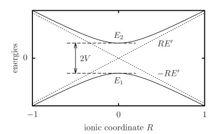
Figure 1: Schematic plot of the diabatic energies $\pm RE^{\prime}$ (dotted lines) and adiabatic energies $E_{1,2}$ (solid lines) in the Landau-Zener model as functions of the ionic distance $R$.

One can also try to generalize the Landau-Zener model to higher dimensions. A simplistic way to achieve this is to promote $E^{\prime}$ to a vector, and, consequently, to interpret $RE^{\prime}$ as a scalar product. In this case Eq. (19) indicates that the direction of $D_{12}$ is along $E^{\prime}$ and $\mu$ is proportional to the tensor product $E^{\prime}\otimes E^{\prime}$. This further supports ansatz (12), with $\hat{\mu}\propto\mathbf{D}_{0}\otimes\mathbf{D}_{0}$, for the NACs, and our findings of Sec. III.4.

V Conclusions

We propose a derivation of the trajectory surface-hopping (TSH) technique based on a semi-classical approximation to the nuclear dynamics in the spirit of a wave packet limit.

The equations governing the electronic transition rates at a simple avoided level crossing display the essential features of TSH algorithm and allows us to elucidate the underlying physics. We find a nonzero electronic transition rate at avoided crossings, which allows for small changes in the nuclear momenta accounted for properly in the energy matching. This justifies the rescaling of the classical velocities done in practice after each hop. Moreover, we find that the physical source of the width of allowed hops in momentum space is related to the speed of variation of the nonadiabatic coupling elements in the adiabatic basis. In the classical limit for the nuclei the derivation supports the rescaling of the momenta along the nonadiabatic coupling vectors. This result strongly relies on the ansatz employed for the nonadiabatic couplings (NACs). In our derivation we assume a multivariate Gaussian form for the NACs, which allows the NACs to fulfill of the so-called curl condition, at least in a two-level case. We also find that the final electronic transition rate is linear in the nonadiabatic coupling vectors, as in the standard TSH algorithm, and that incorporating quantum decoherence makes this scaling quadratic.

Illustration through the Landau-Zener model supports our findings.

Acknowledgments: Work supported by the project RE 322/10-1, Institut Universitaire de France, and Agence Nationale de la Recherche. LS acknowledges financial support from the Spanish MEC (FIS2011-65702-C02-01), ACI-Promociona (ACI2009-1036), Grupos Consolidados UPV/EHU del Gobierno Vasco (IT-319-07), the European Research Council Advanced Grant DYNamo (ERC-2010-AdG-Proposal No. 267374) and CRONOS (280879-2 CRONOS CP-FP7).

Appendix A Gaussian wave packets

In this appendix, we collect a few general properties of the Gaussian wave packets, for which most integrals are known analytically. For example, the folding of Gaussians in general obeys the simple rule

$$\int{\mathrm{d}}^{3N}\mathbf{R} e^{{\mathrm{i}}\mathbf{P}\cdot\mathbf{R}}\,\exp\left(-\frac{(\mathbf{R}^{\prime}-\mathbf{R})^{2}}{a}\right)\,\exp\left(-\frac{{(\mathbf{R}-\mathbf{R}^{\prime\prime})}^{2}}{b}\right)$$ (20)

$$= \left(\frac{ab\pi}{a+b}\right)^{3N/2}\,\exp\left({\mathrm{i}}\mathbf{P}\frac{b\mathbf{R}^{\prime}+a\mathbf{R}^{\prime\prime}}{a+b}\right)$$

$$\exp\left(-\frac{ab}{4(a+b)}\mathbf{P}^{2}-\frac{(\mathbf{R}^{\prime}-\mathbf{R}^{\prime\prime})^{2}}{a+b}\right)\quad.$$

The basic multivariate isotropic Gaussian wave function reads

$$\mathcal{G}_{\mathbf{R}_{i}\mathbf{P}_{i}\lambda}(\mathbf{R})=\left(\frac{\lambda}{\pi}\right)^{3N/4}\exp\left({{\mathrm{i}}}\mathbf{P}_{i}\cdot\mathbf{R}-\frac{\lambda}{2}(\mathbf{R}-\mathbf{R}_{i})^{2}\right)\quad.$$ (21)

where $\lambda$ controls the spatial width of the Gaussian. In the present work we only consider overlaps between two Gaussian wave packets with the same spatial widths and centers,

$$\mathcal{I}_{\mathbf{R}_{i}\lambda}(\mathbf{P}_{i},\mathbf{P}_{j}) = \langle\mathcal{G}_{\mathbf{R}_{i}\mathbf{P}_{i}\lambda}|\mathcal{G}_{\mathbf{R}_{i}\mathbf{P}_{j}\lambda}\rangle$$ (22)

$$= e^{{\mathrm{i}}(\mathbf{P}_{j}-\mathbf{P}_{i})\cdot\mathbf{R}_{i}}\exp\left(-\frac{(\mathbf{P}_{i}-\mathbf{P}_{j})^{2}}{4\lambda}\right)\quad.$$

The inverse of these overlaps, $\mathcal{I}^{-1}_{\mathbf{R}_{i}\lambda}(\mathbf{P}_{k},\mathbf{P}_{j})$ defined to satisfy

$$\int{\mathrm{d}}^{3N}\mathbf{P}_{k}\,\mathcal{I}_{\mathbf{R}_{i}\lambda}(\mathbf{P}_{i},\mathbf{P}_{k})\mathcal{I}^{-1}_{\mathbf{R}_{i}\lambda}(\mathbf{P}_{k},\mathbf{P}_{j})=\delta^{3N}(\mathbf{P}_{i}-\mathbf{P}_{j})\quad,$$ (23)

may be expressed as

$$\mathcal{I}^{-1}_{\mathbf{R}_{i}\lambda}(\mathbf{P}_{i},\mathbf{P}_{j}) = \left(\frac{1}{4\pi\lambda}\right)^{3N/2}e^{-{\mathrm{i}}(\mathbf{P}_{i}-\mathbf{P}_{j})\cdot\mathbf{R}_{i}}$$ (24)

$$\int\frac{{\mathrm{d}}^{3N}\mathbf{Y}}{(2\pi)^{3N}}\exp\left(\lambda\mathbf{Y}^{2}\right)e^{{\mathrm{i}}\mathbf{Y}\cdot(\mathbf{P}_{i}-\mathbf{P}_{j})}\quad.$$

One can verify that such an inverse also satisfies the completeness relation (10).

Details on more general multivariate Gaussians can be found, e.g., in Ref. Riley, Hobson, and Bence, 2006.

Appendix B Proof of the curl-consistency of $\hat{\mu}$ for a two-level system

In the basis where $\hat{\mu}$ is diagonal,

$$\mathbf{D}(\mathbf{R})=\mathbf{D}_{0}\exp\left\{-\sum_{\alpha=1}^{3N}\mu_{\alpha}\left[\left(\mathbf{R}-\mathbf{R}_{\mathrm{c}}\right)_{\alpha}\right]^{2}\right\}\;,$$ (25)

so

$$\frac{\partial D_{\alpha}(\mathbf{R})}{\partial R_{\beta}}-\frac{\partial D_{\beta}(\mathbf{R})}{\partial R_{\alpha}}=-2\left[\mu_{\beta}\left(\mathbf{R}-\mathbf{R}_{\mathrm{c}}\right)_{\beta}D_{\alpha}(\mathbf{R})-\mu_{\alpha}\left(\mathbf{R}-\mathbf{R}_{\mathrm{c}}\right)_{\alpha}D_{\beta}(\mathbf{R})\right]\;.$$ (26)

If we enforce the curl condition for two levels at the point $\mathbf{R}=\mathbf{R}_{\mathrm{c}}+c\hat{\mathbf{e}}_{\gamma}$, where $(\mathbf{R}-\mathbf{R}_{\mathrm{c}})_{\alpha}=c\delta_{\alpha\gamma}$, we get

$$\delta_{\beta\gamma}\mu_{\gamma}D_{0,\alpha}^{(12)}\exp\left(-\mu_{\gamma}c^{2}\right)=\delta_{\alpha\gamma}\mu_{\gamma}D_{0,\beta}^{(12)}\exp\left(-\mu_{\gamma}c^{2}\right)$$ (27)

for all pairs of directions $(\alpha,\beta)$. If we take $\beta=\gamma$, we have

$$\mu_{\gamma}D_{0,\alpha}^{(12)}=\delta_{\alpha\gamma}\mu_{\gamma}D_{0,\gamma}^{(12)}$$ (28)

for all components $\alpha$. There are only two ways to satisfy these equations: either $\mu_{\gamma}=0$, or $D_{0,\alpha}^{(12)}=\delta_{\alpha\gamma}D_{0,\gamma}^{(12)}\;\forall\alpha$. This implies that, if $\gamma$ is a direction such that $\mu_{\gamma}\neq 0$, then, for all components $\alpha\neq\gamma$, $D_{0,\alpha}^{(12)}=0$. Since, in order to have nonzero Gaussian NAC vectors, at least one component of $\mathbf{D}$ and one eigenvalue of $\hat{\mu}$ should be different from zero, there can only be one non-zero eigenvalue of $\hat{\mu}$, and it will correspond to the same direction of the single non-zero component of $\mathbf{D}_{0}^{(12)}$. Therefore, in a base-independent expression, $\hat{\mu}\propto\mathbf{D}_{0}\otimes\mathbf{D}_{0}$, where the tensor product is defined in terms of components as $(a\otimes b)_{\alpha\beta}=a_{\alpha}b_{\beta}$, and the proportionality constant must be a positive real number. It is straightforward that this condition is not only necessary but sufficient, since such a $\hat{\mu}$ will always satisfy Eq. (26).

References

- Born and Huang (2000) M. Born and K. Huang, Dynamical Theory of Crystal Lattices (Oxford University Press, 2000).
- Wodtke, Tully, and Auerbach (2004) A. M. Wodtke, J. C. Tully, and D. J. Auerbach, Int. Rev. in Phys. Chem. 23, 513 (2004).
- Tully and Preston (1971) J. C. Tully and R. K. Preston, J. Chem. Phys. 55, 562 (1971).
- Tully (1990) J. C. Tully, J. Chem. Phys. 93, 1061 (1990).
- Hammes-Schiffer and Tully (1994) S. Hammes-Schiffer and J. C. Tully, J. Chem. Phys. 101, 4657 (1994).
- Webster et al. (1994) F. Webster, E. T. Wang, P. J. Rossky, and R. A. Friesner, J. Chem. Phys. 100, 4835 (1994).
- Tully (1998) J. Tully, Faraday Discuss. 110, 407 (1998).
- Prezhdo and Rossky (1997a) O. Prezhdo and P. Rossky, J. Chem. Phys. 107, 825 (1997a).
- Wong and Rossky (2002a) K. Wong and P. Rossky, J. Chem. Phys. 116, 8418 (2002a).
- Wong and Rossky (2002b) K. Wong and P. Rossky, J. Chem. Phys. 116, 8429 (2002b).
- Bedard-Hearn, Larsen, and Schwartz (2005) M. Bedard-Hearn, R. Larsen, and B. Schwartz, J. Chem. Phys. 123, 234106 (2005).
- Subotnik and Shenvi (2011) J. E. Subotnik and N. Shenvi, J. Chem. Phys. 134, 024105 (2011).
- Subotnik (2011) J. E. Subotnik, J. Phys. Chem. A 115, 12083 (2011).
- Shenvi, Subotnik, and Yang (2011) N. Shenvi, J. E. Subotnik, and W. Yang, J. Chem. Phys. 134, 144102 (2011).
- Hack and Truhlar (2000) M. Hack and D. Truhlar, J. Phys. Chem. A 104, 7917 (2000).
- Herman (1984) M. F. Herman, J. Chem. Phys. 81, 754 (1984).
- Herman (1995) M. F. Herman, J. Chem. Phys. 103, 8081 (1995).
- Wu and Herman (2006) Y. Wu and M. F. Herman, J. Chem. Phys 125, 154116 (2006).
- Schwabl (2007) F. Schwabl, Quantum Mechanics, 4th ed. (Springer, 2007), p. 273–275 .
- Worth and Cederbaum (2004) G. A. Worth and L. S. Cederbaum, Annu. Rev. Phys. Chem. 55, 127 (2004).
- Herman (2001) M. F. Herman, Chem. Phys. 273, 175 (2001).
- Pechukas and Davis (1972) P. Pechukas and J. P. Davis, J. Chem. Phys 56, 4970 (1972).
- Fetter and Walecka (2003) A. Fetter and J. D. Walecka, Quantum Theory of Many-Particle Systems (Dover, 2003).
- Heller (1981) E. J. Heller, J. Chem. Phys. 75, 2923 (1981).
- Schwartz et al. (1996) B. J. Schwartz, E. R. Bittner, O. V. Prezhdo, and P. J. Rossky, J. Chem. Phys. 104, 5942 (1996).
- Neria and Nitzan (1993) E. Neria and A. Nitzan, J. Chem. Phys. 99, 1109 (1993).
- Prezhdo and Rossky (1997b) O. V. Prezhdo and P. J. Rossky, J. Chem. Phys. 107, 5863 (1997b).
- Herman and Kluk (1984) M. F. Herman and E. Kluk, Chem. Phys. 91, 27 (1984).
- Herman, Akramine, and Moody (2004) M. F. Herman, O. E. Akramine, and M. P. Moody, J. Chem. Phys 120, 7383 (2004).
- Prezhdo and Rossky (1998) O. V. Prezhdo and P. J. Rossky, Phys. Rev. Lett. 81, 5294 (1998).
- Baer (2006) M. Baer, Beyond Born-Oppenheimer (John Wiley Sons, 2006).
- Tully (1991) J. C. Tully, Int. J. Quant. Chem. 40, 299 (1991).
- Coker and Xiao (1995) D. F. Coker and L. Xiao, J. Chem. Phys 102, 496 (1995).
- Landry and Subotnik (2011) B. R. Landry and J. E. Subotnik, J. Chem. Phys. 135, 191101 (2011).
- Zener (1932) C. Zener, Proc. Royal Soc. A 137, 696 (1932).
- Riley, Hobson, and Bence (2006) K. F. Riley, M. P. Hobson, and S. J. Bence, Mathematical Methods for Physics and Engineering, 3rd ed. (Cambridge University Press, 2006).