Equivalence of Deterministic One-Counter Automata is NL-complete

Abstract

We prove that language equivalence of deterministic one-counter automata is NL-complete. This improves the superpolynomial time complexity upper bound shown by Valiant and Paterson in 1975. Our main contribution is to prove that two deterministic one-counter automata are inequivalent if and only if they can be distinguished by a word of length polynomial in the size of the two input automata.

1 Introduction

In theoretical computer science, one of the most fundamental decision problems is the equivalence problem which asks whether two given machines behave equivalently. Among the various models of computation – such as Turing machines, random access machines and loop programs, just to mention a few of them – the equivalence problem already becomes undecidable when one imposes strong restrictions on their time and space consumption.

Emerging from formal language theory, a classical model of computation is that of pushdown automata. A folklore result is that already universality (and hence equivalence) of pushdown automata is undecidable. Concerning deterministic pushdown automata (dpda), it is fair to say that the computer science community knows very little about the equivalence problem and its complexity.

Oyamaguchi proved that the equivalence problem for real-time dpda (dpda without $\varepsilon$-transitions) is decidable [17]. It took significant further innovation to show the decidability for general dpda, which is the celebrated result by Sénizergues [19], see also [20]. A couple of years later, Stirling showed that dpda equivalence is in fact primitive recursive [22], and his bound is still the best known upper bound for this problem. Probably due to its intricacy, this fundamental problem has not attracted too much research in the past ten years; only recently a simplified proof has been announced [13], with no substantial improvement of the complexity bound.

It is burdensome to realize that for equivalence of dpda there is still an enormous complexity gap, where the mentioned upper bound is far from the best known lower bound, i.e. from $\mathsf{P}$-hardness (which straightforwardly follows from $\mathsf{P}$-hardness of the emptiness problem).

The same complexity gap persists even for real-time dpda. Thus, further subclasses of dpda have been studied. A $\mathsf{coNP}$ upper bound is known [21] for finite-turn dpda which are dpda where the number of switches between pushing and popping phases is bounded. For simple dpda (which are single state and real-time dpda), equivalence is even decidable in polynomial time [12] (see [4] for the currently best known upper bound).

Deterministic one-counter automata (doca) are one of the simplest infinite-state computational models, extending deterministic finite automata just with one nonnegative integer counter; doca are thus dpda over a singleton stack alphabet plus a bottom stack symbol. Doca were first studied by Valiant and Paterson in 1975 [23]; they showed that equivalence is decidable in time $2^{O(\sqrt{n\log n})}$, and a simple analysis of their proof reveals that the equivalence problem is in $\mathsf{PSPACE}$. The problem is easily shown to be $\mathsf{NL}$-hard, there is however an exponential gap between $\mathsf{NL}$ and $\mathsf{PSPACE}$. There were attempts to settle the complexity of the doca equivalence problem (later we mention some) but the problem proved intricate; only recently $\mathsf{NL}$-completeness was established for real-time one-counter automata [2] but it was far from clear if and how the proof can be extended to the general case.

Let us mention that a convenient and equi-succinct way to present a doca is to partition the control states (and thus the configurations) into stable states, in which the automaton waits for a letter to be read, and into reset states, in which the counter is reset to zero and the residue class of the current counter value modulo some specified number determines the successor (stable) state. Technically speaking, the difference between deterministic one-counter automata and their real-time variant is the lack of reset states in the real-time case. The presence of reset states substantially increases the difficulty of the equivalence problem.

One reason seems to be that a doca can exhibit a behaviour with exponential periodicity, demonstrated by the following example (which slightly adapts the version from [23]). We take a family $(\mathcal{A}_{n})_{n\geq 1}$ where $\mathcal{A}_{n}$ is a doca accepting the regular language $L_{n}=\{a^{m}b_{i}\mid 1\leq i\leq n,m\equiv 0\ (\text{mod }p_{i})\}$, where $p_{i}$ denotes the $i^{\text{th}}$ prime number. The index of the Myhill-Nerode congruence of $L_{n}$ is obviously $2^{\Omega(n)}$ but we can easily construct $\mathcal{A}_{n}$ with $O(n^{2}\log n)$ states. The example also demonstrates that doca are exponentially more succint than their real-time variant, since one can prove that real-time deterministic one-counter automata accepting $L_{n}$ have $2^{\Omega(n)}$ states. It is also easy to show that doca are strictly more expressive than their real-time variant. Analogous expressiveness and succinctness results hold for dpda and real-time dpda, respectively.

As mentioned above, this increase in difficulty in the presence of $\varepsilon$-transitions is confirmed by the fact that it took more than a decade to lift the decidability of real-time dpda [17] to the general case [19, 20].

Our contribution and overview. The main result of this paper is that equivalence of doca is $\mathsf{NL}$-complete, thus closing the exponential complexity gap that has been existing for over thirty-five years ever since doca were introduced.

The above-mentioned exponential behavior of doca is reflected in our central notion of extended deterministic transition system $\mathcal{T}_{\mathsf{ext}}(\mathcal{A})$ that is attached to each doca $\mathcal{A}$. This system includes a special finite deterministic transition system which might be exponentially large in the size of $\mathcal{A}$ and which corresponds to the special-mode variant of stable configurations. Roughly speaking, in the special mode we do not count with reaching the zero value in the counter unless a reset state is visited, and each reset-state visit finishes the special mode. Hence the special mode assumes that the counter is positive and it only requires to remember finite information which is sufficient to perform the resets correctly; in more detail, only the current control state and the current residue classes of the counter value w.r.t. the numbers associated with reset states are needed.

For understanding the shortest words distinguishing two stable inequivalent configurations of $\mathcal{A}$, it turns out useful to include also the special-mode variants of the configurations in the study. This allows us to show that shortest distinguishing words for two zero configurations have polynomial length.

In Section 2 we introduce basic definitions and state our main result that equivalence of doca is $\mathsf{NL}$-complete. A proof of the central claim on polynomial length is given in Section 3 which is in turn divided into the following parts. We give a brief overview of shortest positive paths in the transition system of a doca in Section 3.1; this is the only part which is derived directly from [23]. In Section 3.2 we introduce the above mentioned central notion $\mathcal{T}_{\mathsf{ext}}(\mathcal{A})$, and we make a straightforward analysis of some useful related notions in Sections 3.3–3.7. In particular, in Section 3.4 we study the independence level of a configuration, as the length of a shortest distinguishing word for the configuration and its special-mode variant. This allows us to make various useful observations, e.g. about linear relations between counter values of configurations with the same independence level in Section 3.7.

Sections 3.8 and 3.9 contain the main argument. Sections 3.8 shows that when following a shortest distinguishing word for two zero configurations, we cannot get a long line-climbing segment in which the counter values grow at both sides, keeping a linear relation entailed by keeping the same independence levels. Section 3.9 then shows that a shortest distinguishing word for two zero configurations cannot be long without having a long line-climbing segment.

In Section Appendix (classical doca equivalence) we add a remark on the regularity problem. In Appendix we sketch the standard ideas of showing that the deterministic one-counter automata as introduced in [23] and the above-mentioned reset model that we work with are equi-succinct. We also make clear that our simple form of language equivalence, called trace equivalence, does not bring any loss of generality.

Related work. As mentioned above, doca were introduced by Valiant and Paterson in [23], where the above-mentioned $2^{O(\sqrt{n\log n})}$ time upper bound for language equivalence was proven. Polynomial time algorithms for language equivalence and inclusion for strict subclasses of doca were provided in [10, 11]. In [1, 5] polynomial time learning algorithms were presented for doca. Simulation and bisimulation problems on one-counter automata were studied in [3, 14, 15, 16]. In recent years one-counter automata have attracted a lot of attention in the context of formal verification [9, 7, 6, 8].

Remark: In [1, 18] it is stated that equivalence of doca can be decided in polynomial time. Unfortunately, the proofs provided in [1, 18] were not exact enough to be verified, and they raise several questions which are unanswered to date.

2 Definitions and results

By $\mathbb{N}$ we denote the set $\{0,1,2,\ldots\}$ of non-negative integers, and by $\mathbb{Z}$ the set of all integers. For a finite set $X$, by $|X|$ we denote its cardinality.

By $\Sigma^{*}$ we denote the set of finite sequences of elements of $\Sigma$, i.e. of words over $\Sigma$. For $w\in\Sigma^{*}$, $|w|$ denotes the length of $w$. By $\varepsilon$ we denote the empty word; hence $|\varepsilon|=0$. If $w=uv$ then $u$ is a prefix of $w$ and $v$ is a suffix of $w$.

By $\div$ we denote integer division; for $m,n\in\mathbb{N}$ where $n>0$ we have $m=(m\div n)\cdot n+(m\bmod n)$. We use  “$\bmod$” in two ways, clarified by the following example: $3=18\bmod 5$, $8\neq 18\bmod 5$, $3\equiv 18\,(\bmod\,5)$, $8\equiv 18\,(\bmod\,5)$. For $m\in\mathbb{Z}$, $|m|$ denotes the absolute value of $m$.

We use $\omega$ to stand for infinity; we stipulate $z<\omega$ and $\omega+z=z+\omega=\omega$ for all $z\in\mathbb{Z}$.

A deterministic labelled transition system, a det-LTS for short, is a tuple

$\mathcal{T}=(S_{\mathsf{St}},S_{\varepsilon},\Sigma,(\stackrel{{\scriptstyle a}}{{\mapsto}})_{a\in\Sigma},\stackrel{{\scriptstyle\varepsilon}}{{\mapsto}})$

where $S_{\mathsf{St}}$ and $S_{\varepsilon}$ are (maybe infinite) disjoint sets of stable states and unstable states, respectively, $\Sigma$ is a finite alphabet, $\stackrel{{\scriptstyle a}}{{\mapsto}}\subseteq S_{\mathsf{St}}\times(S_{\mathsf{St}}\cup S_{\varepsilon})$, for $a\in\Sigma$, and $\stackrel{{\scriptstyle\varepsilon}}{{\mapsto}}\subseteq S_{\varepsilon}\times S_{\mathsf{St}}$ are sets of labelled transitions; for each $s\in S_{\varepsilon}$ there is precisely one $t\in S_{\mathsf{St}}$ such that $s\stackrel{{\scriptstyle\varepsilon}}{{\mapsto}}t$, whereas for any $s\in S_{\mathsf{St}}$ and $a\in\Sigma$ there is at most one $t\in S_{\mathsf{St}}\cup S_{\varepsilon}$ such that $s\stackrel{{\scriptstyle a}}{{\mapsto}}t$. For all $w\in\Sigma^{*}$, we define relations $\stackrel{{\scriptstyle w}}{{\longrightarrow}}\subseteq S\times S$, where $S=S_{\mathsf{St}}\cup S_{\varepsilon}$, inductively: $s\stackrel{{\scriptstyle\varepsilon}}{{\longrightarrow}}s$ for each $s\in S$; if $s\stackrel{{\scriptstyle\varepsilon}}{{\mapsto}}t$ then $s\stackrel{{\scriptstyle\varepsilon}}{{\longrightarrow}}t$; if $s\stackrel{{\scriptstyle a}}{{\mapsto}}t$ ($a\in\Sigma$) then $s\stackrel{{\scriptstyle a}}{{\longrightarrow}}t$; if $s\stackrel{{\scriptstyle u}}{{\longrightarrow}}s^{\prime}$ and $s^{\prime}\stackrel{{\scriptstyle v}}{{\longrightarrow}}t$ ($u,v\in\Sigma^{*}$) then $s\stackrel{{\scriptstyle uv}}{{\longrightarrow}}t$.

By $s\stackrel{{\scriptstyle w}}{{\longrightarrow}}$ we denote that $w$ is enabled in $s$, i.e. $s\stackrel{{\scriptstyle w}}{{\longrightarrow}}t$ for some $t$.

Given $\mathcal{T}=(S_{\mathsf{St}},S_{\varepsilon},\Sigma,(\stackrel{{\scriptstyle a}}{{\mapsto}})_{a\in\Sigma},\stackrel{{\scriptstyle\varepsilon}}{{\mapsto}})$, trace equivalence $\sim$ on $S=S_{\mathsf{St}}\cup S_{\varepsilon}$ is defined as follows:

$s\sim t\quad$ if $\quad\forall w\in\Sigma^{*}:s\stackrel{{\scriptstyle w}}{{\longrightarrow}}\,\Leftrightarrow\,t\stackrel{{\scriptstyle w}}{{\longrightarrow}}$.

Hence two states are equivalent iff they enable the same set of words (also called traces). A word $w\in\Sigma^{*}$ is a non-equivalence witness for $(s,t)$, a witness for $(s,t)$ for short, if $w$ is enabled in precisely one of $s,t$.

Remark. By the above definitions, $s\stackrel{{\scriptstyle\varepsilon}}{{\mapsto}}t$ implies $s\sim t$. This could suggest merging the states $s$ and $t$ but we keep them separate since this is convenient in the definitions of det-LTSs generated by deterministic one-counter automata, as given below.

We put $\Sigma^{\leq i}=\{w\in\Sigma^{*};\,|w|\leq i\}$, and we note that $\sim\,=\bigcap\,\{\sim_{i}\mid i\in\mathbb{N}\}$ where the equivalences $\sim_{0}\,\supseteq\,\sim_{1}\,\supseteq\,\sim_{2}\,\supseteq\dots$ are defined as follows:

$s\sim_{i}t\quad$ if $\quad\forall w\in\Sigma^{\leq i}:s\stackrel{{\scriptstyle w}}{{\longrightarrow}}\,\Leftrightarrow\,t\stackrel{{\scriptstyle w}}{{\longrightarrow}}$.

Each pair of states $(s,t)$ has the equivalence level, the eqlevel for short, $\mathsf{EqL}(s,t)\in\mathbb{N}\cup\{\omega\}$:

$\mathsf{EqL}(s,t)=\begin{cases}\omega&\text{ if $s\sim t$},\\ \max\{j\in\mathbb{N}\mid s\sim_{j}t\}&\text{ otherwise.}\end{cases}$

We also write $s\stackrel{{\scriptstyle e}}{{\longleftrightarrow}}t$ instead of $\mathsf{EqL}(s,t)=e$ (where $e\in\mathbb{N}\cup\{\omega\}$). We note that the length of any shortest witness for $(s,t)$, where $s\not\sim t$, is $\mathsf{EqL}(s,t)+1$. We also highlight the next simple fact (valid since our LTSs are deterministic).

Observation 1.

Suppose $s\stackrel{{\scriptstyle w}}{{\longrightarrow}}s^{\prime}$ and $t\stackrel{{\scriptstyle w}}{{\longrightarrow}}t^{\prime}$ in a given det-LTS. Then we have:

1. $\mathsf{EqL}(s^{\prime},t^{\prime})\geq\mathsf{EqL}(s,t)-|w|$. (Hence $s^{\prime}\sim t^{\prime}$ if $s\sim t$.)

2. If $w$ is a (proper) prefix of a witness for $(s,t)$ then $\mathsf{EqL}(s^{\prime},t^{\prime})=\mathsf{EqL}(s,t)-|w|$.

A deterministic one-counter automaton, a doca for short, is a tuple

$\mathcal{A}=(Q_{\mathsf{St}},Q_{\mathsf{Res}},\Sigma,\delta,(\mathsf{per}_{s})_{s\in Q_{\mathsf{Res}}},(\mathsf{goto}_{s})_{s\in Q_{\mathsf{Res}}})$

where $Q_{\mathsf{St}}$ and $Q_{\mathsf{Res}}$ are disjoint finite sets of stable control states and reset control states, respectively, $\Sigma$ is a finite alphabet, $\delta\subseteq Q_{\mathsf{St}}\times\Sigma\times\{0,1\}\times(Q_{\mathsf{St}}\cup Q_{\mathsf{Res}})\times\{-1,0,1\}$ is a set of (transition) rules, $\mathsf{per}_{s}\in\mathbb{N}$ are periods satisfying $1\leq\mathsf{per}_{s}\leq|Q_{\mathsf{St}}|$, and $\mathsf{goto}_{s}:\{0,1,2,\dots,\mathsf{per}_{s}{-}1\}\rightarrow Q_{\mathsf{St}}$ are reset mappings. For each $p\in Q_{\mathsf{St}}$, $a\in\Sigma$, $c\in\{0,1\}$ there is at most one pair $(q,j)$ (where $q\in Q_{\mathsf{St}}\cup Q_{\mathsf{Res}}$, $j\in\{{-}1,0,1\}$) such that $(p,a,c,q,j)\in\delta$; moreover, if $c=0$ then $j\neq{-}1$. The tuples $(p,a,0,q,j)\in\delta$ are called the zero rules, the tuples $(p,a,1,q,j)\in\delta$ are the positive rules.

A doca $\mathcal{A}=(Q_{\mathsf{St}},Q_{\mathsf{Res}},\Sigma,\delta,(\mathsf{per}_{s})_{s\in Q_{\mathsf{Res}}},(\mathsf{goto}_{s})_{s\in Q_{\mathsf{Res}}})$ defines the det-LTS

$$\mathcal{T}(\mathcal{A})=(Q_{\mathsf{St}}\times\mathbb{N},Q_{\mathsf{Res}}\times\mathbb{N},\Sigma,(\stackrel{{\scriptstyle a}}{{\mapsto}})_{a\in\Sigma},\stackrel{{\scriptstyle\varepsilon}}{{\mapsto}})$$ (1)

where $\stackrel{{\scriptstyle a}}{{\mapsto}}$ and $\stackrel{{\scriptstyle\varepsilon}}{{\mapsto}}$ are defined by the following (deduction) rules.

1. If $(p,a,1,q,j)\in\delta$ and $n>0$ then $(p,n)\stackrel{{\scriptstyle a}}{{\mapsto}}(q,n{+}j)$.

2. If $(p,a,0,q,j)\in\delta$ then $(p,0)\stackrel{{\scriptstyle a}}{{\mapsto}}(q,j)$. (Recall that $j\in\{0,1\}$ in this case.)

3. If $s\in Q_{\mathsf{Res}}$ and $n\geq 0$ then $(s,n)\stackrel{{\scriptstyle\varepsilon}}{{\mapsto}}(q,0)$ where $q=\mathsf{goto}_{s}(n\bmod\mathsf{per}_{s})$.

An example of a doca with the respective det-LTS is sketched in Fig. 1.

By a configuration $C$ of the doca $\mathcal{A}$ we mean $(p,m)$, usually written as $p(m)$, where $p$ is its control state and $m\in\mathbb{N}$ is its counter value. If $C=p(0)$ then it is a zero configuration. If $p\in Q_{\mathsf{St}}$ then $C=p(m)$ is a stable configuration; if $p\in Q_{\mathsf{Res}}$ then $p(m)$ is a reset configuration.

Figure 1: A doca $\mathcal{A}$, presented by a graph, and a fragment of $\mathcal{T}(\mathcal{A})$

The definition of (general) det-LTSs induces the relations $\stackrel{{\scriptstyle w}}{{\longrightarrow}}$ ($w\in\Sigma^{*}$) on $Q\times\mathbb{N}$ where $Q=Q_{\mathsf{St}}\cup Q_{\mathsf{Res}}$. We are interested in the doca equivalence problem, denoted

Doca-Eq:

Instance: A doca $\mathcal{A}$ and two stable zero configurations $p(0),q(0)$.

Question: Is $p(0)\sim q(0)$ in $\mathcal{T}(\mathcal{A})$ ?

Our main aim is to show the following theorem.

Theorem 2.

There is a polynomial $\textsc{poly}:\mathbb{N}\rightarrow\mathbb{N}$ such that for any Doca-Eq instance $\mathcal{A},p(0),q(0)$ where $\mathcal{A}$ has $k$ control states we have that $p(0)\not\sim q(0)$ implies $\mathsf{EqL}(p(0),q(0))\leq\textsc{poly}(k)$.

Using Theorem 2, we easily get the next theorem.

Theorem 3.

Doca-Eq is $\mathsf{NL}$-complete.

Proof.

The lower bound follows easily from $\mathsf{NL}$-hardness of digraph reachability.

On the other hand, given a Doca-Eq instance $\mathcal{A},p(0),q(0)$, a nondeterministic algorithm can perform the phases $j=0,1,2,\dots$ described as follows. In phase $j$, there is a pair $(p_{j}(m_{j}),q_{j}(n_{j}))$ in memory, the counter values $m_{j},n_{j}$ written in binary; for $j=0$ we have $(p_{j}(m_{j}),q_{j}(n_{j}))=(p(0),q(0))$. If $\mathsf{EqL}(p_{j}(m_{j}),q_{j}(n_{j}))>0$ then a letter $a$ is nondeterministically chosen, and $(p_{j}(m_{j}),q_{j}(n_{j}))$ is replaced with $(p_{j+1}(m_{j+1}),q_{j+1}(n_{j+1}))$ where $p_{j}(m_{j})\stackrel{{\scriptstyle a}}{{\longrightarrow}}p_{j+1}(m_{j+1})$ and $q_{j}(m_{j})\stackrel{{\scriptstyle a}}{{\longrightarrow}}q_{j+1}(m_{j+1})$.

If $p(0)\not\sim q(0)$ then Theorem 2 guarantees that a pair $(p_{j}(m_{j}),q_{j}(n_{j}))$ with $\mathsf{EqL}(p_{j}(m_{j}),q_{j}(n_{j}))=0$ can be thus reached by using only logarithmic space.

Hence Doca-Eq is in co-$\mathsf{NL}$. Since $\mathsf{NL}$$=$co-$\mathsf{NL}$, we are done. ∎

3 Proof of Theorem 1

Convention. When considering a doca $\mathcal{A}$, we will always tacitly assume the notation

$$\mathcal{A}=(Q_{\mathsf{St}},Q_{\mathsf{Res}},\Sigma,\delta,(\mathsf{per}_{s})_{s\in Q_{\mathsf{Res}}},(\mathsf{goto}_{s})_{s\in Q_{\mathsf{Res}}})$$ (2)

if not said otherwise. We also reserve $k$ for denoting the number of control states, i.e.

$k=|Q_{\mathsf{St}}|+|Q_{\mathsf{Res}}|$.

To be more concise in the later reasoning concerning a given doca $\mathcal{A}$, we use the words “few”, “small”, or “short” when we mean that the relevant quantity is bounded by a polynomial in $k$; the polynomial is always independent of $\mathcal{A}$. By a small rational number we mean $\rho=\frac{a}{b}$ or $\rho=-\frac{a}{b}$ where $a,b\in\mathbb{N}$ are small. We also say that

a set is small if its cardinality is a small number.

We note that if all elements of a set $X$ of (integer or rational) numbers are small then $X$ is a small set; the opposite is not true in general. We often tacitly use the fact that

a quantity arising as the sum or the product of two small quantities is also small.

Though these expressions might look informal, they can be always easily replaced by the formal statements which they abridge. By this convention, Theorem 2 says that the eqlevel of any pair of zero configurations is small when finite.

Remark. It will be always obvious that we could calculate a concrete respective polynomial whenever we use “few”, “small”, “short” in our claims. But such calculations would add tedious technicalities, and they would be not particularly rewarding w.r.t. the degree of the polynomials. We thus prefer a transparent concise proof which avoids technicalities whenever possible.

3.1 Shortest positive paths in $\mathcal{T}(\mathcal{A})$

We first define the notion of paths in general det-LTSs, and then we look at special paths in $\mathcal{T}(\mathcal{A})$, for a doca $\mathcal{A}$.

Definition 4.

Given a det-LTS $\mathcal{T}=(S_{\mathsf{St}},S_{\varepsilon},\Sigma,(\stackrel{{\scriptstyle a}}{{\mapsto}})_{a\in\Sigma},\stackrel{{\scriptstyle\varepsilon}}{{\mapsto}})$, a path in $\mathcal{T}$ is a sequence

$s_{0}\stackrel{{\scriptstyle a_{1}}}{{\longrightarrow}}s_{1}\stackrel{{\scriptstyle a_{2}}}{{\longrightarrow}}\dots\stackrel{{\scriptstyle a_{z}}}{{\longrightarrow}}s_{z}$ ($z\in\mathbb{N}$)

where $s_{i}\in S_{\mathsf{St}}$ and $a_{i}\in\Sigma$ (for all $i,0\leq i\leq z$); it is a path from its start $s_{0}$ to its end $s_{z}$. For any $i_{1},i_{2}$, where $0\leq i_{1}\leq i_{2}\leq z$, the sequence $s_{i_{1}}\stackrel{{\scriptstyle a_{i_{1}+1}}}{{\longrightarrow}}s_{i_{1}+1}\stackrel{{\scriptstyle a_{i_{1}+2}}}{{\longrightarrow}}\cdots\stackrel{{\scriptstyle a_{i_{2}}}}{{\longrightarrow}}s_{i_{2}}$ is a subpath of the above path. Slightly abusing notation, we will also use $s\stackrel{{\scriptstyle w}}{{\longrightarrow}}$ and $s\stackrel{{\scriptstyle w}}{{\longrightarrow}}t$ ($s,t\in S_{\mathsf{St}}$) to denote paths.

We also refer to $s\stackrel{{\scriptstyle a}}{{\longrightarrow}}t$ where $s,t\in S_{\mathsf{St}}$ and $a\in\Sigma$ as to a step. If $s\stackrel{{\scriptstyle a}}{{\mapsto}}t$ then it is a simple step; if $s\stackrel{{\scriptstyle a}}{{\mapsto}}s^{\prime}\stackrel{{\scriptstyle\varepsilon}}{{\mapsto}}t$ then it is a combined step. The length of a path $s_{0}\stackrel{{\scriptstyle a_{1}}}{{\longrightarrow}}s_{1}\stackrel{{\scriptstyle a_{2}}}{{\longrightarrow}}\dots\stackrel{{\scriptstyle a_{z}}}{{\longrightarrow}}s_{z}$ is $z$, i.e. the number of its steps.

When discussing the det-LTS $\mathcal{T}(\mathcal{A})$ for a doca $\mathcal{A}$, we use the term reset steps instead of combined steps. We now concentrate on positive paths in $\mathcal{T}(\mathcal{A})$, defined as follows.

Definition 5.

Given a doca $\mathcal{A}$ (in notation (2)), a path

$$p_{0}(m_{0})\stackrel{{\scriptstyle a_{1}}}{{\longrightarrow}}p_{1}(m_{1})\stackrel{{\scriptstyle a_{2}}}{{\longrightarrow}}\cdots\stackrel{{\scriptstyle a_{z}}}{{\longrightarrow}}p_{z}(m_{z})$$ (3)

in $\mathcal{T}(\mathcal{A})$ is positive if each step $p_{i}(m_{i})\stackrel{{\scriptstyle a_{i+1}}}{{\longrightarrow}}p_{i+1}(m_{i+1})$ ($0\leq i<z$) is simple and is induced by a positive rule $(p_{i},a_{i+1},1,p_{i+1},j)\in\delta$ (where $j=m_{i+1}{-}m_{i}$).

The effect (or the counter change) of the path (3) is $m_{z}{-}m_{0}$; if the path is positive, its effect is an integer in the interval $[{-}z,z]$. The path (3) is a control state cycle if it is positive and we have $z>0$ and $p_{z}=p_{0}$.

We note that if (3) is positive then there is no reset step in the path and $m_{i}>0$ for all $i,0\leq i<z$; but we can have $m_{z}=0$.

The next lemma can be easily derived from Lemma $2$ in [23]; we thus only sketch the idea. The claim of the lemma is illustrated in Fig. 2.

Figure 2: Shortest positive paths in $\mathcal{T}(\mathcal{A})$, one from a configuration $C_{1}$ to $C_{2}$ and one from $C_{2}$ to a zero configuration $C_{3}$. (Only the stable control states $q_{1},q_{2},\dots,q_{k_{1}}$ are depicted.)

Lemma 6.

If there is a positive path from $p(m)$ to $q(n)$ in $\mathcal{T}(\mathcal{A})$ then some of the shortest positive paths from $p(m)$ to $q(n)$ is of the form

$p(m)\stackrel{{\scriptstyle u_{1}}}{{\longrightarrow}}p^{\prime}(m^{\prime})\stackrel{{\scriptstyle v^{i}}}{{\longrightarrow}}p^{\prime}(m^{\prime}{+}id)\stackrel{{\scriptstyle u_{2}}}{{\longrightarrow}}q(n)$

where $u_{1}$ is a short word, called the pre-phase, $p^{\prime}(m^{\prime})\stackrel{{\scriptstyle v}}{{\longrightarrow}}p^{\prime}(m^{\prime}{+}d)$ is a short control state cycle with the effect $d\in\mathbb{Z}$, and $u_{2}$ is a short word, called the post-phase. (The cycle $v$ is repeated $i$ times, where $i\geq 0$.)

Proof.

(Sketch.) Lemma $2$ in [23] considers the case when $m\geq n+k^{2}$. The cycle $v$ shown by that lemma has the length in $\{1,2,\dots,k\}$ and the effect in $\{-1,-2,\dots,-k\}$. The length of the pre-phase plus the post-phase is bounded by $k^{2}$. The idea is to use a most effective control state cycle for repeating (with the largest ratio $\frac{|\text{effect}|}{\text{length}}$), and to add the “cost” of reaching that cycle from $p(m)$ and of reaching $q(n)$ from the end of the repeated cycle. The technical details can be found in [23].

The situation with $n\geq m+k^{2}$ is handled symmetrically. Having solved the case $|n-m|\geq k^{2}$, the case $|n-m|<k^{2}$ is obvious, as can be seen in Fig. 2: if a long path is going up via a short cycle with a positive effect $d_{1}$ and then down via another short cycle with a negative effect $-d_{2}$, then it can be shortened by removing $d_{2}$ copies of the first cycle and $d_{1}$ copies of the second cycle. Hence $|n-m|<k^{2}$ implies that there is a short positive path $p(m)\stackrel{{\scriptstyle u_{1}}}{{\longrightarrow}}q(n)$ (with $v=u_{2}=\varepsilon$). ∎

It is useful to highlight the following corollary of the previous lemma.

Corollary 7.

If $|m-n|$ is small and there is a positive path from $p(m)$ to $q(n)$ then there is a short positive path from $p(m)$ to $q(n)$.

3.2 The extended det-LTS $\mathcal{T}_{\mathsf{ext}}(\mathcal{A})$

We now introduce a central notion, the det-LTS $\mathcal{T}_{\mathsf{ext}}(\mathcal{A})$, which extends the det-LTS $\mathcal{T}(\mathcal{A})$ defined in (1), for a given doca $\mathcal{A}=(Q_{\mathsf{St}},Q_{\mathsf{Res}},\Sigma,\delta,(\mathsf{per}_{s})_{s\in Q_{\mathsf{Res}}},(\mathsf{goto}_{s})_{s\in Q_{\mathsf{Res}}})$.

Before giving a formal definition, we give an intuitive explanation. Let us (temporarily) imagine that $\mathcal{A}$ has also a special mode of behaviour, besides the normal mode defined previously; let any configuration $p(m)$ have its special-mode analogue $\overline{p}(m)$. For any positive counter value $m>0$, each transition $p(m)\stackrel{{\scriptstyle a}}{{\mapsto}}q(m{+}j)$ ($a\in\Sigma$) induces the transition $\overline{p}(m)\stackrel{{\scriptstyle a}}{{\mapsto}}\overline{q}(m{+}j)$. Further, any transition $s(m)\stackrel{{\scriptstyle\varepsilon}}{{\mapsto}}q(0)$ ($s\in Q_{\mathsf{Res}}$, $m\geq 0$) induces $\overline{s}(m)\stackrel{{\scriptstyle\varepsilon}}{{\mapsto}}q(0)$; hence the special mode is finished by any reset step, after which the normal mode applies. A crucial property of the special mode is that whenever a configuration $\overline{p}(0)$, where $p\in Q_{\mathsf{St}}$, is entered (by a non-reset step), a multiple (the least common multiple, say) $\Delta\in\mathbb{N}$ of all periods $\mathsf{per}_{s}$, $s\in Q_{\mathsf{Res}}$, is silently added to the counter (we put $\Delta=1$ when $Q_{\mathsf{Res}}=\emptyset$). Hence the zero rules are never used in the special mode since the counter is always positive (until a possible reset step is performed). If we added the special-mode configurations and the respective transitions to $\mathcal{T}(\mathcal{A})$, we would easily observe that

• $p(m)\sim_{m}\overline{p}(m)$ (thus $\mathsf{EqL}(p(m),\overline{p}(m))\geq m$);

• $p(m)\not\sim\overline{p}(m)$ iff there is a positive path $p(m)\stackrel{{\scriptstyle u}}{{\longrightarrow}}q(0)$ (and thus $\overline{p}(m)\stackrel{{\scriptstyle u}}{{\longrightarrow}}\overline{q}(0)=\overline{q}(\Delta)$)
  for some $q\in Q_{\mathsf{St}}$ such that $q(0)\not\sim\overline{q}(0)$ (i.e. $q(0)\not\sim\overline{q}(\Delta)$);

• if $m\equiv m^{\prime}\,(\bmod\,\mathsf{per}_{s})$ for all $s\in Q_{\mathsf{Res}}$ then $\overline{p}(m)\sim\overline{p}(m^{\prime})$;

• if $s\in Q_{\mathsf{Res}}$ and $m\equiv m^{\prime}\,(\bmod\,\mathsf{per}_{s})$ then $\overline{s}(m)\sim\overline{s}(m^{\prime})$.

In the special mode of $\mathcal{A}$, the concrete value $m$ of the counter is not important once we know the tuple $(c_{s})_{s\in Q_{\mathsf{Res}}}$ where $c_{s}=m\bmod\mathsf{per}_{s}$; in a reset configuration $\overline{s}(m)$, knowing just $c=m\bmod\mathsf{per}_{s}$ is sufficient.

We do not formalize the above notions and claims, since they only serve us for a better understanding of the definition of $\mathcal{T}_{\mathsf{ext}}(\mathcal{A})$ given below. The det-LTS $\mathcal{T}_{\mathsf{ext}}(\mathcal{A})$ arises from $\mathcal{T}(\mathcal{A})$ by adding a finite set $Q_{\mathsf{Mod}}$ of stable states and a finite set $Q_{\mathsf{FixRes}}$ of unstable states and the transitions defined below. The transitions from $Q_{\mathsf{Mod}}$ will only lead to $Q_{\mathsf{Mod}}\cup Q_{\mathsf{FixRes}}$, whereas the $\varepsilon$-transitions from $Q_{\mathsf{FixRes}}$ lead to zero configurations in $\mathcal{T}(\mathcal{A})$. There are no transitions leading from the configurations in $\mathcal{T}(\mathcal{A})$ to $Q_{\mathsf{Mod}}\cup Q_{\mathsf{FixRes}}$, and the subgraph of $\mathcal{T}_{\mathsf{ext}}(\mathcal{A})$ arising by the restriction to the configurations of $\mathcal{T}(\mathcal{A})$ is $\mathcal{T}(\mathcal{A})$ itself. We thus also safely use the same symbols $\stackrel{{\scriptstyle a}}{{\mapsto}}$, $\stackrel{{\scriptstyle\varepsilon}}{{\mapsto}}$ in both $\mathcal{T}(\mathcal{A})$ and $\mathcal{T}_{\mathsf{ext}}(\mathcal{A})$. An example is sketched in Fig. 3.

Figure 3: A fragment of $\mathcal{T}_{\mathsf{ext}}(\mathcal{A})$ where: $\{p,q,r\}\subseteq Q_{\mathsf{St}}$, $Q_{\mathsf{Res}}=\{s,s^{\prime},s^{\prime\prime},s^{\prime\prime\prime}\}$, $\{a,b,c\}\subseteq\Sigma$, $\{(p,a,1,q,-1),(p,b,1,s^{\prime},0),(p,c,1,p,1)\}\subseteq\delta$, $(\mathsf{per}_{s},\mathsf{per}_{s^{\prime}},\mathsf{per}_{s^{\prime\prime}},\mathsf{per}_{s^{\prime\prime\prime}})=(7,4,6,8)$, $\mathsf{goto}_{s^{\prime}}(1)=r$, $\Delta=lcm\{7,4,6,8\}=168$.

Definition 8.

Given a doca $\mathcal{A}=(Q_{\mathsf{St}},Q_{\mathsf{Res}},\Sigma,\delta,(\mathsf{per}_{s})_{s\in Q_{\mathsf{Res}}},(\mathsf{goto}_{s})_{s\in Q_{\mathsf{Res}}})$, with the associated det-LTS  $\mathcal{T}(\mathcal{A})=(Q_{\mathsf{St}}\times\mathbb{N},Q_{\mathsf{Res}}\times\mathbb{N},\Sigma,(\stackrel{{\scriptstyle a}}{{\mapsto}})_{a\in\Sigma},\stackrel{{\scriptstyle\varepsilon}}{{\mapsto}})$, we define the det-LTS

$\mathcal{T}_{\mathsf{ext}}(\mathcal{A})=((Q_{\mathsf{St}}\times\mathbb{N})\cup Q_{\mathsf{Mod}},(Q_{\mathsf{Res}}\times\mathbb{N})\cup Q_{\mathsf{FixRes}},\Sigma,(\stackrel{{\scriptstyle a}}{{\mapsto}})_{a\in\Sigma},\stackrel{{\scriptstyle\varepsilon}}{{\mapsto}})$

as the extension of $\mathcal{T}(\mathcal{A})$ where

• $Q_{\mathsf{Mod}}=\{(p,(c_{s})_{s\in Q_{\mathsf{Res}}})\mid p\in Q_{\mathsf{St}},0\leq c_{s}\leq\mathsf{per}_{s}-1\}$,

• $Q_{\mathsf{FixRes}}=\{s_{[c]}\mid s\in Q_{\mathsf{Res}},0\leq c\leq\mathsf{per}_{s}-1\}$, and

• the additional transitions are defined by the following (deduction) rules:

  1. If $(p,a,1,q,j)\in\delta$ and $q\in Q_{\mathsf{St}}$ then for each $(p,(c_{s})_{s\in Q_{\mathsf{Res}}})\in Q_{\mathsf{Mod}}$ we have

     $(p,(c_{s})_{s\in Q_{\mathsf{Res}}})\stackrel{{\scriptstyle a}}{{\mapsto}}(q,(c^{\prime}_{s})_{s\in Q_{\mathsf{Res}}})$

     where $c^{\prime}_{s}=(c_{s}{+}j)\bmod\mathsf{per}_{s}$ for each $s\in Q_{\mathsf{Res}}$.

  2. If $(p,a,1,s^{\prime},j)\in\delta$ and $s^{\prime}\in Q_{\mathsf{Res}}$ then for each $(p,(c_{s})_{s\in Q_{\mathsf{Res}}})\in Q_{\mathsf{Mod}}$ we have

     $(p,(c_{s})_{s\in Q_{\mathsf{Res}}})\stackrel{{\scriptstyle a}}{{\mapsto}}s^{\prime}_{[c]}$

     where $c=(c_{s^{\prime}}{+}j)\bmod\mathsf{per}_{s^{\prime}}$.

  3. For each $s_{[c]}\in Q_{\mathsf{FixRes}}$ we have $s_{[c]}\stackrel{{\scriptstyle\varepsilon}}{{\mapsto}}q(0)$ where $q=\mathsf{goto}_{s}(c)$.

A configuration $C$ is a state in $\mathcal{T}_{\mathsf{ext}}(\mathcal{A})$. If $C\in Q_{\mathsf{Mod}}$ or $C=p(m)$ where $p\in Q_{\mathsf{St}}$ then $C$ is stable, otherwise $C$ is unstable.

Moreover, we define the mapping

$\mathsf{Mod}:((Q_{\mathsf{St}}\cup Q_{\mathsf{Res}})\times\mathbb{N})\rightarrow(Q_{\mathsf{Mod}}\cup Q_{\mathsf{FixRes}})$:

• if $p\in Q_{\mathsf{St}}$ then $\mathsf{Mod}(p(m))=(p,(c_{s})_{s\in Q_{\mathsf{Res}}})\in Q_{\mathsf{Mod}}$ where $c_{s}=m\bmod\mathsf{per}_{s}$ for all $s\in Q_{\mathsf{Res}}$;

• if $s\in Q_{\mathsf{Res}}$ then $\mathsf{Mod}(s(m))=s_{[c]}\in Q_{\mathsf{FixRes}}$ where $c=m\bmod\mathsf{per}_{s}$.

We note that the cardinality of $Q_{\mathsf{Mod}}$ might be exponential in $k$ (i.e. in the number of control states of $\mathcal{A}$). On the other hand, $Q_{\mathsf{FixRes}}$ is small; this is a crucial fact for some claims in the next auxiliary propositions. We stipulate $\min\emptyset=\omega$, and recall that $z+\omega=\omega$ for any $z\in\mathbb{N}$.

Proposition 9.

1. If $(p,(c_{s})_{s\in Q_{\mathsf{Res}}})\stackrel{{\scriptstyle w}}{{\longrightarrow}}(q,(c^{\prime}_{s})_{s\in Q_{\mathsf{Res}}})$ then for each $(p,(d_{s})_{s\in Q_{\mathsf{Res}}})\in Q_{\mathsf{Mod}}$ we have $(p,(d_{s})_{s\in Q_{\mathsf{Res}}})\stackrel{{\scriptstyle w}}{{\longrightarrow}}(q,(d^{\prime}_{s})_{s\in Q_{\mathsf{Res}}})$ where $d^{\prime}_{s}{-}c^{\prime}_{s}\equiv d_{s}{-}c_{s}\,(\bmod\ \mathsf{per}_{s})$ for all $s\in Q_{\mathsf{Res}}$.

2. If $(p,(c_{s})_{s\in Q_{\mathsf{Res}}})\stackrel{{\scriptstyle w}}{{\longrightarrow}}s^{\prime}_{[c]}$ then for each $(p,(d_{s})_{s\in Q_{\mathsf{Res}}})\in Q_{\mathsf{Mod}}$ we have $(p,(d_{s})_{s\in Q_{\mathsf{Res}}})\stackrel{{\scriptstyle w}}{{\longrightarrow}}s^{\prime}_{[d]}$ where $d{-}c\equiv d_{s^{\prime}}{-}c_{s^{\prime}}\,(\bmod\,\mathsf{per}_{s^{\prime}})$.

3. For any $s\in Q_{\mathsf{Res}}$ we have $s(m)\sim\mathsf{Mod}(s(m))$.

4. If $p\in Q_{\mathsf{St}}$ then $\mathsf{EqL}(p(m),\mathsf{Mod}(p(m)))=$
   $=\min\{z+\mathsf{EqL}(q(0),\mathsf{Mod}(q(0)))\mid q\in Q_{\mathsf{St}}$ and $z$ is the length of a positive path from $p(m)$ to $q(0)\}$.

5. For any $p\in Q_{\mathsf{St}}$, $m\in\mathbb{N}$, and $w\in\Sigma^{*}$ there is some small positive $d\in\mathbb{N}$ such that

   • either for each $m^{\prime}$ such that $m^{\prime}\equiv m\,(\bmod\,d)$ we have that $\mathsf{Mod}(p(m^{\prime}))$ enables $w$,

   • or for each $m^{\prime}$ such that $m^{\prime}\equiv m\,(\bmod\,d)$ we have that $\mathsf{Mod}(p(m^{\prime}))$ does not enable $w$.

Proof.

Points 1 and 2 can be easily shown by induction on $|w|$, using Def. 8.

Point 3 is obvious since $s(m)\stackrel{{\scriptstyle\varepsilon}}{{\mapsto}}q(0)$ and $\mathsf{Mod}(s(m))\stackrel{{\scriptstyle\varepsilon}}{{\mapsto}}q(0)$ for the appropriate $q\in Q_{\mathsf{St}}$.

Point 4:

We first note that if $p(m)\stackrel{{\scriptstyle w}}{{\longrightarrow}}q(n)$ is a positive path (in $\mathcal{T}(\mathcal{A})$) then we have $\mathsf{Mod}(p(m))\stackrel{{\scriptstyle w}}{{\longrightarrow}}\mathsf{Mod}(q(n))$ (as can be easily shown by induction on $|w|$).

One part of the equality, namely $\mathsf{EqL}(p(m),\mathsf{Mod}(p(m)))\leq\min\{\dots\}$, is thus clear; it remains to show

$$\mathsf{EqL}(p(m),\mathsf{Mod}(p(m)))\geq\min\{z+\mathsf{EqL}(q(0),\mathsf{Mod}(q(0)))\mid\dots\}.$$ (4)

The case where $p(m)\sim\mathsf{Mod}(p(m))$ is trivial. We thus further consider only the cases $p(m)\not\sim\mathsf{Mod}(p(m))$, and we proceed by induction on $\mathsf{EqL}(p(m),\mathsf{Mod}(p(m)))$. If $\mathsf{EqL}(p(m),\mathsf{Mod}(p(m)))=0$ then we obviously must have $m=0$, and (4) is trivial in any case with $m=0$.

Let us now assume $m>0$, and let $av$ ($a\in\Sigma$) be a shortest witness for $(p(m),\mathsf{Mod}(p(m)))$. We must have some $(p,a,1,q,j)\in\delta$, and thus $p(m)\stackrel{{\scriptstyle a}}{{\mapsto}}q(m{+}j)$ and $\mathsf{Mod}(p(m))\stackrel{{\scriptstyle a}}{{\mapsto}}\mathsf{Mod}(q(m{+}j))$ (as can be easily checked). Point 3 excludes the case $q\in Q_{\mathsf{Res}}$, hence $q\in Q_{\mathsf{St}}$. By recalling Observation 1(2), and using the induction hypothesis for $q(m+j),\mathsf{Mod}(q(m+j))$, we finish the proof easily: $\mathsf{EqL}(p(m),\mathsf{Mod}(p(m)))=1+\mathsf{EqL}(q(m{+}j),\mathsf{Mod}(q(m{+}j)))\geq 1+z+\mathsf{EqL}(q^{\prime}(0),\mathsf{Mod}(q^{\prime}(0)))$ where $z$ is the length of some positive path from $q(m{+}j)$ to $q^{\prime}(0)$, and $1{+}z$ is thus the length of some positive path from $p(m)$ to $q^{\prime}(0)$.

Point 5:

By recalling Points 1 and 2, we easily note the following fact:
If $\mathsf{Mod}(p(m_{1}))\stackrel{{\scriptstyle u}}{{\longrightarrow}}C\in Q_{\mathsf{Mod}}\cup Q_{\mathsf{FixRes}}$ then for any $m_{2}$ there is $C^{\prime}\in Q_{\mathsf{Mod}}\cup Q_{\mathsf{FixRes}}$ such that $\mathsf{Mod}(p(m_{2}))\stackrel{{\scriptstyle u}}{{\longrightarrow}}C^{\prime}$; moreover, if $\mathsf{Mod}(p(m_{1}))\stackrel{{\scriptstyle u}}{{\longrightarrow}}s_{[c]}$ then $\mathsf{Mod}(p(m_{2}))\stackrel{{\scriptstyle u}}{{\longrightarrow}}s_{[c]}$ for any $m_{2}$ such that $m_{2}\equiv m_{1}\,(\bmod\,\mathsf{per}_{s})$.

Hence if $w=uv$ where $\mathsf{Mod}(p(m))\stackrel{{\scriptstyle u}}{{\longrightarrow}}s_{[c]}$ then the claim is satisfied by $d=\mathsf{per}_{s}$, and otherwise it is satisfied even by $d=1$. ∎

We recall that $C\stackrel{{\scriptstyle e}}{{\longleftrightarrow}}C^{\prime}$ means $\mathsf{EqL}(C,C^{\prime})=e$.

Proposition 10.

1. For any $p,q\in Q_{\mathsf{St}}$ and $m,n\in\mathbb{N}$ there are small positive $d_{1},d_{2}\in\mathbb{N}$ such that for any $m^{\prime},n^{\prime}\in\mathbb{N}$ we have: if $m^{\prime}\equiv m\,(\bmod\,d_{1})$ and $n^{\prime}\equiv n\,(\bmod\,d_{2})$ then

   $\mathsf{EqL}(\mathsf{Mod}(p(m^{\prime})),\mathsf{Mod}(q(n^{\prime})))\leq\mathsf{EqL}(\mathsf{Mod}(p(m)),\mathsf{Mod}(q(n)))$.

2. The set $\{\,e\mid\text{ there are }C,C^{\prime}\in Q_{\mathsf{Mod}}\text{ s.t. }C\stackrel{{\scriptstyle e}}{{\longleftrightarrow}}C^{\prime}\}$ is small.

Proof.

Point 1:
If $\mathsf{Mod}(p(m))\sim\mathsf{Mod}(q(n))$ then the claim is trivial. We thus assume $\mathsf{Mod}(p(m))\not\sim\mathsf{Mod}(q(n))$ and let $w$ be a shortest witness for $(\mathsf{Mod}(p(m)),\mathsf{Mod}(q(n)))$.

By Prop. 9(5), $p,m,w$ give rise to $d_{1}$ and $q,n,w$ give rise to $d_{2}$ such that precisely one of $\mathsf{Mod}(p(m^{\prime})),\mathsf{Mod}(q(n^{\prime}))$ enables $w$ when $m^{\prime}\equiv m\,(\bmod\,d_{1})$ and $n^{\prime}\equiv n\,(\bmod\,d_{2})$. In this case $w$ is a witness (not necessarily a shortest) for $(\mathsf{Mod}(p(m^{\prime})),\mathsf{Mod}(q(n^{\prime})))$, and the claim thus follows.

Point 2:
It is obvious that the set in Point 2 is equal to

$\{\,e\mid\mathsf{Mod}(p(m))\stackrel{{\scriptstyle e}}{{\longleftrightarrow}}\mathsf{Mod}(q(n))$ for some $p,q\in Q_{\mathsf{St}},m,n\in\mathbb{N}\}$.

With every tuple $(p,m,q,n)$ we associate a fixed tuple $(d_{1},d_{2},c_{1},c_{2})$ where $d_{1},d_{2}$ are those guaranteed by Point 1, and $c_{1}=m\bmod d_{1}$, $c_{2}=n\bmod d_{2}$. If two tuples $(p,m_{1},q,n_{1})$, $(p,m_{2},q,n_{2})$ have the same associated tuple $(d_{1},d_{2},c_{1},c_{2})$ then $\mathsf{EqL}(\mathsf{Mod}(p(m_{1})),\mathsf{Mod}(q(n_{1})))=\mathsf{EqL}(\mathsf{Mod}(p(m_{2})),\mathsf{Mod}(q(n_{2})))$, as follows by applying Point 1 in both directions. Since the number of possible tuples $(p,q,d_{1},d_{2},c_{1},c_{2})$ is small, we are done. ∎

The next proposition can be proved analogously as the previous one.

Proposition 11.

1. For any $p,q\in Q_{\mathsf{St}}$ and $m,n\in\mathbb{N}$ there is some small positive $d\in\mathbb{N}$ such that for any $m^{\prime}\in\mathbb{N}$ we have: if $m^{\prime}\equiv m\,(\bmod\,d)$ then

   $\mathsf{EqL}(\mathsf{Mod}(p(m^{\prime})),q(n))\leq\mathsf{EqL}(\mathsf{Mod}(p(m)),q(n))$.

2. For any (fixed) $q(n)$, the set $\{\,e\mid\text{ there is }C\in Q_{\mathsf{Mod}}\text{ s.t. }C\stackrel{{\scriptstyle e}}{{\longleftrightarrow}}q(n)\}$ is small.

3.3 Eqlevels of pairs of zero configurations

Let us recall $\mathcal{T}_{\mathsf{ext}}(\mathcal{A})$ defined in Def. 8. We could view the elements of $Q_{\mathsf{Mod}}\cup Q_{\mathsf{FixRes}}$ as additional control states of $\mathcal{A}$; in these states the counter value would play no role and could be formally viewed as zero. This observation justifies the name “zero configurations” in the following definition.

Definition 12.

Given a doca $\mathcal{A}$ as in (2), with the associated $\mathcal{T}_{\mathsf{ext}}(\mathcal{A})$ by Def. 8, a state $C$ in $\mathcal{T}_{\mathsf{ext}}(\mathcal{A})$ is a zero configuration if either $C\in Q_{\mathsf{Mod}}\cup Q_{\mathsf{FixRes}}$ or $C=p(0)$ where $p\in Q_{\mathsf{St}}\cup Q_{\mathsf{Res}}$.

We define the set $\textsc{ZE}\subseteq\mathbb{N}$ (Zero configurations Eqlevels) as follows:

$\textsc{ZE}=\{\,e\in\mathbb{N}\mid$ there are two stable zero configurations $C,C^{\prime}$ s.t. $C\stackrel{{\scriptstyle e}}{{\longleftrightarrow}}C^{\prime}\}$.

We thus have $\textsc{ZE}=\textsc{E}_{1}\cup\textsc{E}_{2}\cup\textsc{E}_{3}$ where

$\textsc{E}_{1}=\{\,e\in\mathbb{N}\mid p(0)\stackrel{{\scriptstyle e}}{{\longleftrightarrow}}q(0)$ for some $p,q\in Q_{\mathsf{St}}\}$,

$\textsc{E}_{2}=\{\,e\in\mathbb{N}\mid p(0)\stackrel{{\scriptstyle e}}{{\longleftrightarrow}}C$ for some $p\in Q_{\mathsf{St}},C\in Q_{\mathsf{Mod}}\}$,

$\textsc{E}_{3}=\{\,e\in\mathbb{N}\mid C\stackrel{{\scriptstyle e}}{{\longleftrightarrow}}C^{\prime}$ for some $C,C^{\prime}\in Q_{\mathsf{Mod}}\}$.

Since the set $\{\,p(0)\mid p\in Q_{\mathsf{St}}\}$ is obviously small, by Prop. 10(2) and 11(2) we easily derive the following claim.

Lemma 13.

The set ZE is small.

The lemma does not claim that the elements of ZE are small numbers. This will be shown in the following subsections; i.e., we will prove the next theorem which strengthens Theorem 2.

Theorem 14.

There is a polynomial $\textsc{poly}:\mathbb{N}\rightarrow\mathbb{N}$ such that $\max\,\{\,e\mid e\in\textsc{ZE}\}\leq\textsc{poly}(k)$ (for any doca $\mathcal{A}$ with $k$ control states).

Let $e_{0}<e_{1}<e_{2}<\dots<e_{f}$ be the ordered elements of ZE. We have shown that $f$ is small but we have not yet shown that all $e_{i}$ are small numbers. W.l.o.g. we can assume $e_{0}=0$ (by adding two special control states, say). For proving Theorem 14 it thus suffices to show that the “gaps” between $e_{i}$ and $e_{i+1}$, i.e. the differences $e_{i+1}{-}e_{i}$, are small. We will later contradict the existence of a large gap between $e_{i}=e_{D}$ (Down) and $e_{i+1}=e_{U}$ (Up) depicted in Figure 4.

$e_{0}--e_{1}-\dots-e_{D}-----------------e_{U}-\dots-e_{f}$

Figure 4: Assumption of a large gap in ZE (to be contradicted later)

But we first explore some further notions related to a given doca $\mathcal{A}$ and the det-LTS $\mathcal{T}_{\mathsf{ext}}(\mathcal{A})$.

3.4 Independence level

We assume a doca $\mathcal{A}$ as in (2), and explore a notion which we have already touched on implicitly.

Definition 15.

For $p\in Q_{\mathsf{St}}$, $m\in\mathbb{N}$ we put

$\mathsf{IL}(p(m))=\mathsf{EqL}(p(m),\mathsf{Mod}(p(m)))$.

$\mathsf{IL}(p(m))$ can be understood as an “Independence Level” of $p(m)$ w.r.t. the concrete value $m$.

Proposition 16.

For each $p(m)$ with $\mathsf{IL}(p(m))<\omega$ there are small rational numbers $\rho$, $\sigma$ (of the type $\frac{a}{b}$, $-\frac{a}{b}$ where $a,b\in\mathbb{N}$ are small) and some $q\in Q_{\mathsf{St}}$ such that

$\mathsf{IL}(p(m))=\rho\cdot m+\sigma+\mathsf{IL}(q(0))$.

Moreover, we can require $\rho\geq 0$, $\rho\cdot m+\sigma\geq 0$, and if $m$ is larger than a small bound then $\rho>0$.

Convention. We will further assume that each $p(m)$ with $\mathsf{IL}(p(m))<\omega$ has a fixed associated equality $\mathsf{IL}(p(m))=\rho\cdot m+\sigma+e$ where $e=\mathsf{IL}(q(0))\in\textsc{ZE}$ and $\rho,\sigma,q$ have the claimed properties.

Proof.

Suppose $\mathsf{IL}(p(m))<\omega$. If $m=0$ then we can take $\rho=\sigma=0$ and $q=p$. If $m>0$ then Prop. 9(4) implies that there is some $q\in Q_{\mathsf{St}}$ such that $\mathsf{IL}(p(m))=|w|+\mathsf{IL}(q(0))$ where $p(m)\stackrel{{\scriptstyle w}}{{\longrightarrow}}q(0)$ is a shortest positive path from $p(m)$ to $q(0)$. (Recall the path from $C_{2}$ to $C_{3}$ in Fig. 2 as an example.) By Lemma 6 we can assume that $w$ is in the form $u_{1}v^{i}u_{2}$, for a short prefix $u_{1}$, a short repeated cycle $v$, and a short suffix $u_{2}$. Hence $|w|=i\cdot|v|+|u_{1}|+|u_{2}|$, and $m=i\cdot(-d)-d_{1}-d_{2}$ where $d,d_{1},d_{2}$ are the effects of (i.e. the counter changes caused by) $v,u_{1},u_{2}$, respectively. We note that $d_{2}\leq 0$ and that we can assume $d<0$. Since $i=\frac{m+d_{1}+d_{2}}{-d}$, we get $|w|=\frac{|v|}{-d}\cdot m+\frac{|v|\cdot(d_{1}+d_{2})}{-d}+|u_{1}|+|u_{2}|$. As $\mathsf{IL}(p(m))=|w|+\mathsf{IL}(q(0))$, all the claims follow easily. ∎

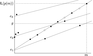
Figure 5 depicts $\mathsf{IL}(p(m))$ for a fixed $p\in Q_{\mathsf{St}}$ and for a few values $m$, by using black circles $\bullet$; $e_{1},e_{2},e_{3}$ are elements of ZE corresponding to $\mathsf{IL}(q(0))$ for several $q$. There might be some “irregular” values $\mathsf{IL}(p(m))=z+\mathsf{IL}(q(0))$ for small $m$ and small $z$ but for $m$ larger than a small bound the values $\mathsf{IL}(p(m))$ lie on few lines, starting near some $e_{j}$ and having small slopes. (In fact, we have $1\leq\frac{|v|}{|\mathsf{effect}(v)|}\leq k$ for the respective cycles $v$ in $w=u_{1}v^{i}u_{2}$; the unit-length for the vertical axis is thus smaller than for the horizontal axis in Fig. 5.) The circles $\bullet$ and $\circ$ on one depicted line can correspond to the pairs $(m_{0},z_{0}+\mathsf{IL}(q(0)))$, $(m_{0}+d,z_{0}+d^{\prime}+\mathsf{IL}(q(0)))$, $(m_{0}+2d,z_{0}+2d^{\prime}+\mathsf{IL}(q(0)))$, $\dots$ where $d=|\mathsf{effect}(v)|$ and $d^{\prime}=|v|$ (and $z_{0}=|u_{1}u_{2}|$, $z_{0}+d^{\prime}=|u_{1}vu_{2}|$, $z_{0}+2d^{\prime}=|u_{1}v^{2}u_{2}|$, $\dots$). A white circle $\circ$ depicts that the respective value, corresponding to a positive path $p(m_{0}{+}id)\stackrel{{\scriptstyle u_{1}v^{i}u_{2}}}{{\longrightarrow}}q(0)$, is not $\mathsf{IL}(p(m_{0}{+}id))$ since there is another, and shorter, witness in this case.

Figure 5: Illustrating $\mathsf{IL}(p(m))$ as a function of $m$

We now observe some further facts for later use.

Proposition 17.

1. For each $g\in\mathbb{N}$ there are only few $p(m)$ such that $\mathsf{IL}(p(m))=g$.

2. For any $p(m)$ where $\mathsf{IL}(p(m))<\omega$ there are some small numbers $\mathsf{base}\geq 0$ and $\mathsf{per}>0$ such that the following condition holds:
   for any $m^{\prime}$ such that $\mathsf{base}\leq m^{\prime}<m$ and $m^{\prime}\equiv m\,(\bmod\ \mathsf{per})$ we have $\mathsf{IL}(p(m^{\prime}))<\mathsf{IL}(p(m))$.

Proof.

Point 1 is intuitively clear from the horizontal line at level $g$ in Fig. 5. Formally, we look when we can have $g=\rho\cdot m+\sigma+e$ where $\mathsf{IL}(p(m))=\rho\cdot m+\sigma+e$ is the equality associated with some $p(m)$ (by Convention after Prop. 16). Since there are only few possibilities for $\rho,\sigma,e$, and we can have $\rho=0$ only for few (small) values $m$, there are only few possible $m$ which might fit.

Point 2 has been intuitively shown by the line with black and white circles in Fig. 5 and by the respective discussion. To be more formal, we recall that $\mathsf{IL}(p(m))=|w|+\mathsf{IL}(q(0))$ for some $q\in Q_{\mathsf{St}}$ and a shortest positive path $p(m)\stackrel{{\scriptstyle w}}{{\longrightarrow}}q(0)$ from $p(m)$ to $q(0)$. We assume $w=u_{1}v^{i}u_{2}$ for short $u_{1},v,u_{2}$ as in the proof of Prop. 16. Hence if $m$ is bigger than a small bound then $i>0$. Let $\mathsf{per}=|\mathsf{effect}(v)|$. Then we have

$p(m-\mathsf{per})\xrightarrow{u_{1}v^{i-1}u_{2}}q(0)$,

$p(m-2\cdot\mathsf{per})\xrightarrow{u_{1}v^{i-2}u_{2}}q(0)$,

$\dots$,

$p(m-x\cdot\mathsf{per})\xrightarrow{u_{1}v^{i-x}u_{2}}q(0)$

for $x=(m{-}\mathsf{base})\div\mathsf{per}$ where we put $\mathsf{base}=|u_{1}|{+}|u_{2}|{+}|v|$ to be safe, i.e. to guarantee that $u_{1}v^{i-j}u_{2}$ is indeed enabled in $p(m-j\cdot\mathsf{per})$, for all $j=1,2,\dots,x$. Since $p(m-j\cdot\mathsf{per})\xrightarrow{u_{1}v^{i-j}u_{2}}q(0)$ is a positive path, we have $\mathsf{IL}(p(m-j\cdot\mathsf{per}))\leq|u_{1}v^{i-j}u_{2}|+\mathsf{IL}(q(0))$ by Prop. 9(4). Since $|u_{1}v^{i-j}u_{2}|+\mathsf{IL}(q(0))<|w|+\mathsf{IL}(q(0))=\mathsf{IL}(p(m)$, we are done. ∎

3.5 Eqlevel tuples

We introduce the eqlevel tuples illustrated in Fig. 6, assuming a given doca $\mathcal{A}$ as in (2), with the associated det-LTSs $\mathcal{T}(\mathcal{A})$ and $\mathcal{T}_{\mathsf{ext}}(\mathcal{A})$. A simple property of these tuples considerably simplifies the later analysis.

Figure 6: Eqlevel tuple $(b,\ell,r,o,d^{L},d^{R})$ associated to a pair $(p(m),q(n))$, and to a pair $(p(m),C)$ where $C\in Q_{\mathsf{Mod}}$

Definition 18.

Each pair $(p(m),q(n))$ of stable configurations in $\mathcal{T}(\mathcal{A})$ has the associated eqlevel tuple $(b,\ell,r,o,d^{L},d^{R})$ (of elements from $\mathbb{N}\cup\{\omega\}$) defined as follows:

• $b=\mathsf{EqL}(p(m),q(n))$ (Basic),

• $\ell=\mathsf{IL}(p(m))$ (Left),

• $r=\mathsf{IL}(q(n))$ (Right),

• $o=\mathsf{EqL}(\mathsf{Mod}(p(m)),\mathsf{Mod}(q(n))$ (mOd),

• $d^{L}=\mathsf{EqL}(p(m),\mathsf{Mod}(q(n))$ (Diagonal Left),

• $d^{R}=\mathsf{EqL}(q(n),\mathsf{Mod}(p(m))$ (Diagonal Right).

Each pair $(p(m),C)$ where $C\in Q_{\mathsf{Mod}}$ and $p(m)$ is a stable configuration in $\mathcal{T}(\mathcal{A})$ has the associated eqlevel tuple $(b,\ell,r,o,d^{L},d^{R})$ defined as follows:

• $b=d^{L}=\mathsf{EqL}(p(m),C)$,

• $\ell=\mathsf{IL}(p(m))$,

• $r=\omega$,

• $o=d^{R}=\mathsf{EqL}(\mathsf{Mod}(p(m)),C)$.

We could similarly associate a tuple to $(C,q(n))$ but this is not needed in later reasoning. The following trivial fact yields an important corollary for the eqlevel tuples; it holds for general LTSs but we confine ourselves to the introduced det-LTSs.

Proposition 19.

Given states $s_{1},s_{2},\dots,s_{m}$ in a det-LTS where $m\geq 2$ and $s_{1}\stackrel{{\scriptstyle e_{1}}}{{\longleftrightarrow}}s_{2}$, $s_{2}\stackrel{{\scriptstyle e_{2}}}{{\longleftrightarrow}}s_{3}$, $\dots$, $s_{m-1}\stackrel{{\scriptstyle e_{m-1}}}{{\longleftrightarrow}}s_{m}$, $s_{m}\stackrel{{\scriptstyle e_{m}}}{{\longleftrightarrow}}s_{1}$, the minimum of $\{e_{1},e_{2},\dots,e_{m}\}$ cannot be $e_{i}$ for just one $i$.

Proof.

We assume by contradiction that $\min\{e_{1},\ldots,e_{m}\}=e_{i}$ for just one $i\in\{1,\ldots,m\}$; w.l.o.g. we assume $i=1$, and we note that $e_{1}<\omega$ (since $m\geq 2$). Then we have $s_{2}\sim_{e_{1}+1}s_{3}\sim_{e_{1}+1}s_{4}\,\cdots\sim_{e_{1}+1}s_{m}\sim_{e_{1}+1}s_{1}$ and hence $s_{1}\sim_{e_{1}+1}s_{2}$ by transitivity and symmetry of $\sim_{e_{1}+1}$; this contradicts the assumption $s_{1}\stackrel{{\scriptstyle e_{1}}}{{\longleftrightarrow}}s_{2}$. ∎

Corollary 20.

In the “triangle” $(b,\ell,d^{R})$, we always have $b=\ell$ or $b=d^{R}$ or $\ell=d^{R}$ (or $b=\ell=d^{R}$) as the minimum. Similarly for the “triangles” $(d^{R},r,o)$, $(b,d^{L},r)$, and $(\ell,d^{L},o)$. In the “rectangle” $(b,\ell,r,o)$, the minimum is also achieved by at least two elements (concretely by $b=\ell$, $b=r$, $b=o$, $\ell=r$, $\ell=o$, or $r=o$).

3.6 Paths in $\mathcal{T}(\mathcal{A})\times\mathcal{T}(\mathcal{A})$

Since we are interested in comparing two states in a det-LTS $\mathcal{T}$, it is useful to define the product $\mathcal{T}\times\mathcal{T}$; the transitions in $\mathcal{T}\times\mathcal{T}$ are just the letter-synchronized pairs of transitions in $\mathcal{T}$. Eqlevel-decreasing paths in $\mathcal{T}\times\mathcal{T}$ will be of particular interest. A formal definition follows.

Definition 21.

Let $\mathcal{T}=(S_{\mathsf{St}},S_{\varepsilon},\Sigma,(\stackrel{{\scriptstyle a}}{{\mapsto}})_{a\in\Sigma},\stackrel{{\scriptstyle\varepsilon}}{{\mapsto}})$ be a det-LTS. We define the det-LTS

$\mathcal{T}\times\mathcal{T}=(S_{\mathsf{St}}\times S_{\mathsf{St}},S^{\prime}_{\varepsilon},\Sigma,(\stackrel{{\scriptstyle a}}{{\mapsto}})_{a\in\Sigma},\stackrel{{\scriptstyle\varepsilon}}{{\mapsto}})$

where $S^{\prime}_{\varepsilon}=(S_{\mathsf{St}}\times S_{\varepsilon})\cup(S_{\varepsilon}\times S_{\mathsf{St}})\cup(S_{\varepsilon}\times S_{\varepsilon})$ and the transitions are defined as follows:

1. If $s,t\in S_{\mathsf{St}}$ and $s\stackrel{{\scriptstyle a}}{{\mapsto}}s^{\prime}$ and $t\stackrel{{\scriptstyle a}}{{\mapsto}}t^{\prime}$ (for $a\in\Sigma$) then $(s,t)\stackrel{{\scriptstyle a}}{{\mapsto}}(s^{\prime},t^{\prime})$.

2. If $s\in S_{\mathsf{St}}$, $t\in S_{\varepsilon}$, and $t\stackrel{{\scriptstyle\varepsilon}}{{\mapsto}}t^{\prime}$ then $(s,t)\stackrel{{\scriptstyle\varepsilon}}{{\mapsto}}(s,t^{\prime})$.

3. If $s\in S_{\varepsilon}$, $t\in S_{\mathsf{St}}$, and $s\stackrel{{\scriptstyle\varepsilon}}{{\mapsto}}s^{\prime}$ then $(s,t)\stackrel{{\scriptstyle\varepsilon}}{{\mapsto}}(s^{\prime},t)$.

4. If $s\stackrel{{\scriptstyle\varepsilon}}{{\mapsto}}s^{\prime}$ and $t\stackrel{{\scriptstyle\varepsilon}}{{\mapsto}}t^{\prime}$ then $(s,t)\stackrel{{\scriptstyle\varepsilon}}{{\mapsto}}(s^{\prime},t^{\prime})$.

A path $(s_{0},s^{\prime}_{0})\stackrel{{\scriptstyle a_{1}}}{{\longrightarrow}}(s_{1},s^{\prime}_{1})\stackrel{{\scriptstyle a_{2}}}{{\longrightarrow}}(s_{2},s^{\prime}_{2})$ $\,\cdots$ $\stackrel{{\scriptstyle a_{z}}}{{\longrightarrow}}(s_{z},s^{\prime}_{z})$ in $\mathcal{T}\times\mathcal{T}$ (where $(s_{i},s^{\prime}_{i})\in S_{\mathsf{St}}\times S_{\mathsf{St}}$ by Def. 4) is eqlevel-decreasing if $\mathsf{EqL}(s_{i},s^{\prime}_{i})>\mathsf{EqL}(s_{i+1},s^{\prime}_{i+1})$ for all $i\in\{0,1,,\dots,z{-}1\}$.

We can easily verify that $\mathcal{T}\times\mathcal{T}$ is indeed a det-LTS. We also note that in eqlevel-decreasing paths we must have $\mathsf{EqL}(s_{i+1},s^{\prime}_{i+1})=\mathsf{EqL}(s_{i},s^{\prime}_{i})-1$, by Observation 1. We also observe:

Observation 22.

1. Any subpath of an eqlevel-decreasing path in $\mathcal{T}\times\mathcal{T}$ is a shortest path from its start to its end.

2. Suppose the path $(s,t)\stackrel{{\scriptstyle w}}{{\longrightarrow}}(s^{\prime},t^{\prime})$ is eqlevel-decreasing. If $(s,t)\stackrel{{\scriptstyle v}}{{\longrightarrow}}(s^{\prime\prime},t^{\prime\prime})$ where $|v|<|w|$ then $\mathsf{EqL}(s^{\prime\prime},t^{\prime\prime})>\mathsf{EqL}(s^{\prime},t^{\prime})$.

We now look at $\mathcal{T}(\mathcal{A})\times\mathcal{T}(\mathcal{A})$ for a doca $\mathcal{A}$.

Definition 23.

We call $(p(m),q(n))\stackrel{{\scriptstyle a}}{{\longrightarrow}}(p^{\prime}(m^{\prime}),q^{\prime}(n^{\prime}))$ a reset step (in $\mathcal{T}(\mathcal{A})\times\mathcal{T}(\mathcal{A})$) if at least one of component-steps $p(m)\stackrel{{\scriptstyle a}}{{\longrightarrow}}p^{\prime}(m^{\prime})$, $q(n)\stackrel{{\scriptstyle a}}{{\longrightarrow}}q^{\prime}(n^{\prime})$ is a reset step in $\mathcal{T}(\mathcal{A})$. If precisely one of component-steps is a reset step then $(p(m),q(n))\stackrel{{\scriptstyle a}}{{\longrightarrow}}(p^{\prime}(m^{\prime}),q^{\prime}(n^{\prime}))$ is a one-side reset step, if both component-steps are reset steps then $(p(m),q(n))\stackrel{{\scriptstyle a}}{{\longrightarrow}}(p^{\prime}(m^{\prime}),q^{\prime}(n^{\prime}))$ is a both-side reset step.

We note that one of $m^{\prime},n^{\prime}$ is $0$ when $(p(m),q(n))\stackrel{{\scriptstyle a}}{{\longrightarrow}}(p^{\prime}(m^{\prime}),q^{\prime}(n^{\prime}))$ is a one-side reset step, and $m^{\prime}=n^{\prime}=0$ when it is a both-side reset step.

Figure 7: A path from $(p(0),q(0))$ in $\mathcal{T}(\mathcal{A})\times\mathcal{T}(\mathcal{A})$ (with some one-side resets), projected to $\mathbb{N}\times\mathbb{N}$.

Fig. 7 shows an example of a path $\mathcal{T}(\mathcal{A})\times\mathcal{T}(\mathcal{A})$, projected to $\mathbb{N}\times\mathbb{N}$ (a pair $(p(m),q(n))$ is projected to $(m,n)$); the dotted lines represent one-side reset steps. Theorem 2 claims, in fact, that the eqlevel-decreasing paths in $\mathcal{T}(\mathcal{A})\times\mathcal{T}(\mathcal{A})$ which start from pairs of zero configurations are short.

3.7 $\mathsf{IL}$-equality lines

We assume a fixed doca $\mathcal{A}$, and consider the cases $\mathsf{IL}(p(m))=\mathsf{IL}(q(n))<\omega$ (i.e., $\ell=r<\omega$ in Fig. 6); we explore what we can say about the respective points $(m,n)\in\mathbb{N}\times\mathbb{N}$. By Convention after Prop. 16, each such case has the associated equalities $\mathsf{IL}(p(m))=\rho\cdot m+\sigma+e$ and $\mathsf{IL}(q(n))=\rho^{\prime}\cdot n+\sigma^{\prime}+e^{\prime}$, and $\mathsf{IL}(p(m))=\mathsf{IL}(q(n))$ thus implies $\rho\cdot m+\sigma+e=\rho^{\prime}\cdot n+\sigma^{\prime}+e^{\prime}$.

Only in few cases we have $\rho=0$ or $\rho^{\prime}=0$ (which is clear by Prop. 16 and Prop. 17(1)); in the other (many) cases we have $n=\frac{\rho}{\rho^{\prime}}m+\frac{(\sigma{-}\sigma^{\prime})+(e-e^{\prime})}{\rho^{\prime}}$ where $\frac{\rho}{\rho^{\prime}}>0$. This naturally leads to the following notions (illustrated in Fig. 8).

Figure 8: A sketch of $\mathsf{IL}$-equality lines (in reality, lines contain only points with integer coordinates)

Definition 24.

A pair $(\mu,\tau)$ of rational numbers is a valid slope-shift pair if there are some $p(m)$, $q(n)$ with the associated equalities $\mathsf{IL}(p(m))=\rho\cdot m+\sigma+e$ and $\mathsf{IL}(q(n))=\rho^{\prime}\cdot n+\sigma^{\prime}+e^{\prime}$ such that $\rho\cdot m+\sigma+e=\rho^{\prime}\cdot n+\sigma^{\prime}+e^{\prime}$, $\rho>0$, $\rho^{\prime}>0$, $\mu=\frac{\rho}{\rho^{\prime}}$, $\tau=\frac{(\sigma{-}\sigma^{\prime})+(e-e^{\prime})}{\rho^{\prime}}$.

Each valid slope-shift pair $(\mu,\tau)$ defines an $\mathsf{IL}$-equality line, or just a line for short, namely the set $\{(x,y)\in\mathbb{N}\times\mathbb{N}\mid y=\mu\cdot x+\tau\}$.

Any maximal set of parallel lines (having the same slope but various shifts) is a line-bunch. (The maximality is taken w.r.t. set inclusion.) We say that $(x,y)\in\mathbb{N}\times\mathbb{N}$ is in a line-bunch $H$ if $(x,y)$ is in a line in $H$.

Though each line contains at least one $(m,n)$ such that $\mathsf{IL}(p(m))=\mathsf{IL}(q(n))<\omega$ for some $p,q$, the definition does not assume anything more specific about lines. The line-bunches can have various “gaps”, and if a point $(x,y)$ is not in a line-bunch $H$ then it can still lie between two lines from $H$. The following proposition is easy to verify.

Proposition 25.

1. There are only few lines, and thus also few line-bunches.
   The set $\{(x,y)\in\mathbb{N}\times\mathbb{N}\mid(x,y)\in L_{1}\cap L_{2}$ for two different lines $L_{1},L_{2}\}$ is small.

2. There are only few pairs $(p(m),q(n))$ where $\mathsf{IL}(p(m))=\mathsf{IL}(q(n))<\omega$ and $(m,n)$ is not in a line.

3.8 Eqlevel-decreasing line-climbing paths are short

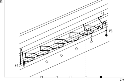
We recall Fig. 4 which assumes a large gap $e_{U}{-}e_{D}$; to finish a proof of Theorem 14, we aim to show that all gaps in ZE are, in fact, small. In the next subsection (3.9) we show that a large gap $e_{U}{-}e_{D}$ would entail a long eqlevel-decreasing line-climbing path in $\mathcal{T}(\mathcal{A})\times\mathcal{T}(\mathcal{A})$ (depicted in Fig. 9). In this subsection we show that all such paths are, in fact, short. Fig. 9 illustrates a line-climbing path from a pair projected to $P_{1}$ to a larger pair projected to $P_{2}$. The cyclicity and further structures in the figure will be discussed later.

Figure 9: A line-climbing path (projections of all visited configuration-pairs are in IL-equality lines in one line-bunch)

Definition 26.

A path in $\mathcal{T}(\mathcal{A})\times\mathcal{T}(\mathcal{A})$ is positive if each pair $(p(m),q(n))$ in the path satisfies $m>0$, $n>0$; this entails that there are no reset steps in the path.

A positive path $(p_{0}(m_{0}),q_{0}(n_{0}))\stackrel{{\scriptstyle a_{1}}}{{\longrightarrow}}$ $(p_{1}(m_{1}),q_{1}(n_{1}))\stackrel{{\scriptstyle a_{2}}}{{\longrightarrow}}$ $\cdots$ $\stackrel{{\scriptstyle a_{z}}}{{\longrightarrow}}(p_{z}(m_{z}),q_{z}(n_{z}))$ is line-climbing if $m_{0}<m_{z}$ and all $(m_{i},n_{i})$, for $i=0,1,2,\dots,z$, are in one line-bunch.

We do not require that $(m_{0},n_{0})$ and $(m_{z},n_{z})$ are in the same line, and we might have $n_{z}\leq n_{0}$; hence “line-climbing” might be understood as a shorthand for “(left-to-right) line-bunch climbing”.

To get some intuition for what follows, imagine that Fig. 9 illustrates the projection of a “cyclic” line-climbing eqlevel-decreasing path from $P_{1}$ to $P_{2}$ which is followed by a simple step leading out of the respective line-bunch, namely to the black-diamond point. Cutting off the copies of the cycle in the path would give rise to the sequence of white-diamond points.

Fig. 9 also illustrates a similar path from $P_{1}$ to $P^{\prime}_{2}$ which is followed by another type of leaving the line-bunch, namely by a one-side reset step to the black-box point. Cutting off the copies of the cycle in the path would now give rise to the sequence of white-box points.

If the original path, including the line-bunch leaving step, is eqlevel-decreasing then the eqlevel of the “exit pair” (the black diamond or the black box) is less than the eqlevels of all “earlier exit pairs” (white diamonds or white boxes) (recall Observation 22(2)). The sequence of white-diamond (or white-box) points, finished by the black-diamond (or black-box) point, inspires the following definition.

Definition 27.

For $p,q\in Q_{\mathsf{St}}$, a sequence of pairs

$(p(m_{0}),q(n_{0})),(p(m_{1}),q(n_{1})),(p(m_{2}),q(n_{2})),\dots,(p(m_{z}),q(n_{z}))$

where $z\geq 1$ is strange periodic if the following conditions hold:

1. $(m_{i},n_{i})=(m_{0}+i\cdot c_{1},n_{0}+i\cdot c_{2})$ for some $c_{1},c_{2}\in\mathbb{N}$ and $i=0,1,\dots,z$;

2. $\mathsf{EqL}(p(m_{i}),q(n_{i}))>\mathsf{EqL}(p(m_{z}),q(n_{z}))$ for all $i\in\{0,1,\dots,z{-}1\}$ (hence $c_{1}>0$ or $c_{2}>0$);

3. the pairs $(m_{0},n_{0}),(m_{1},n_{1}),\dots,(m_{z},n_{z})$ are not all in one $\mathsf{IL}$-equality line.

Prop. 25 implies that in any strange periodic sequence there are only few pairs $(p(m_{i}),q(n_{i}))$ such that $\mathsf{IL}(p(m_{i}))=\mathsf{IL}(q(n_{i}))<\omega$.

We now show that all strange periodic sequences are short, and then we derive that all line-climbing eqlevel-decreasing paths are short. (Fig. 9 suggests that such paths can be assumed to use a “cycle”; this will be established later by another use of Lemma 6.)

Proposition 28.

Strange periodic sequences are short.

Proof.

Let us assume a strange periodic sequence

$$(p(m_{0}),q(n_{0})),(p(m_{1}),q(n_{1})),(p(m_{2}),q(n_{2})),\dots,(p(m_{z}),q(n_{z}))$$ (5)

as in Def. 27. Hence there are $c_{1},c_{2}\in\mathbb{N}$ such that $(m_{i},n_{i})=(m_{0}+i\cdot c_{1},n_{0}+i\cdot c_{2})$ for $i=0,1,\dots,z$; moreover, $c_{1}>0$ or $c_{2}>0$, and the pairs in (5) are thus pairwise different.

For $i\in\{0,1,\dots,z\}$, by

$(b_{i},\ell_{i},r_{i},o_{i},d^{L}_{i},d^{R}_{i})$ we denote the eqlevel tuple associated with $(p(m_{i}),q(n_{i}))$

(recall Fig. 6 and Cor. 20). As we already noted, we have

$$\ell_{i}=r_{i}<\omega\textnormal{ only for few }i\in\{0,1,2,\dots,z\}.$$ (6)

We now explore certain “dense” periodic subsequences of (5). By a periodic subsequence, with the period $\mathsf{per}>0$ and the base $b\geq 0$, we mean the sequence of pairs $(p(m_{j}),q(n_{j}))$ where $j$ ranges over the index set

$\mathcal{J}=\{z-x\cdot\mathsf{per},z-(x{-}1)\cdot\mathsf{per},z-(x{-}2)\cdot\mathsf{per},\dots,z-2\cdot\mathsf{per},z-\mathsf{per}\}$

for $x=(z{-}b)\div\mathsf{per}$. If both $b$ and $\mathsf{per}$ are small (i.e., bounded by $\textsc{poly}(k)$ for a fixed polynomial poly independent of the assumed doca $\mathcal{A}$ with $k$ control states) then we say that this periodic subsequence is dense. We note that

if a dense subsequence is short then the whole sequence (5) is short (i.e., $z$ is small).

By (2) in Def. 27 we have $b_{i}>b_{z}$ for all $i<z$, hence also $b_{j}>b_{z}$ for all $j\in\mathcal{J}$ where $\mathcal{J}$ is the index set of a periodic subsequence. Using Prop. 17(2), we now observe that there is a dense subsequence, with the index set $\mathcal{J}_{1}$, where $\ell_{j}\leq\ell_{z}$ for all $j\in\mathcal{J}_{1}$ (when $\ell_{z}<\omega$ and $c_{1}>0$ then we can even establish $\ell_{j}<\ell_{z}$). Similarly there is a dense subsequence, with the index set $\mathcal{J}_{2}$, where $r_{j}\leq r_{z}$ for all $j\in\mathcal{J}_{2}$. By using Prop. 10(1) we derive that there is also a dense subsequence, with the index set $\mathcal{J}_{3}$, where $o_{j}\leq o_{z}$ for all $j\in\mathcal{J}_{3}$. (Given $d_{1},d_{2}$ guaranteed for $p,q,m_{z},n_{z}$ by Prop. 10(1), we can take $d_{1}\cdot d_{2}$ as the period of the subsequence.)

Moreover, if $c_{2}=0$, and thus $q(n_{i})=q(n_{0})$ in all pairs in (5), then Prop. 11(1) implies that there is a dense subsequence, with the index set $\mathcal{J}_{4}$, where $d^{R}_{j}\leq d^{R}_{z}$ for all $j\in\mathcal{J}_{4}$.

We now perform a case analysis.

1. $c_{1}>0$, $c_{2}=0$ (the case $c_{1}=0$, $c_{2}>0$ is symmetric)

   Here we have $q(n_{i})=q(n_{0})$ in all pairs in (5). Considering the triangle $\{b_{z},\ell_{z},d^{R}_{z}\}$ (recall Fig. 6 and Cor. 20), we note that we must have $\ell_{z}\leq b_{z}<\omega$ or $d^{R}_{z}\leq b_{z}<\omega$. Hence there is a dense subsequence, indexed by $\mathcal{J}$, where $\ell_{j}\leq\ell_{z}\leq b_{z}<b_{j}$ for all $j\in\mathcal{J}$, or $d^{R}_{j}\leq d^{R}_{z}\leq b_{z}<b_{j}$ for all $j\in\mathcal{J}$. In both cases, Cor. 20 implies that $\ell_{j}=d^{R}_{j}<b_{j}$ for all $j\in\mathcal{J}$. Since each $d^{R}_{j}$ belongs to the set $\{\,e\mid\mathsf{Mod}(p(m))\stackrel{{\scriptstyle e}}{{\longleftrightarrow}}q(n_{0})$ for some $m\,\}$, Prop. 11(2) implies that the set $\{d^{R}_{j}\mid j\in\mathcal{J}\}=\{\ell_{j}\mid j\in\mathcal{J}\}$ is small. Prop. 17(1) then implies that the set $\{p(m_{0}+j\cdot c_{1})\mid j\in\mathcal{J}\}$ is small; this implies that $\mathcal{J}$ is small and thus (5) is short.

2. $c_{1}>0$, $c_{2}>0$

   Looking at the rectangle $\{b_{z},\ell_{z},r_{z},o_{z}\}$, we note that we have $\ell_{z}\leq b_{z}<\omega$ or $r_{z}\leq b_{z}<\omega$ or $o_{z}\leq b_{z}<\omega$. Hence there is a dense subsequence, indexed by $\mathcal{J}$, where $\ell_{j}\leq\ell_{z}\leq b_{z}<b_{j}$ for all $j\in\mathcal{J}$, or $r_{j}\leq r_{z}\leq b_{z}<b_{j}$ for all $j\in\mathcal{J}$, or $o_{j}\leq o_{z}\leq b_{z}<b_{j}$ for all $j\in\mathcal{J}$. In any case, Cor. 20 implies that for each $j\in\mathcal{J}$ we have $\ell_{j}=r_{j}<\omega$ or $\ell_{j}=o_{j}<\omega$ or $r_{j}=o_{j}<\omega$.

   We note that the set $\{(p(m_{0}+j\cdot c_{1}),q(n_{0}+j\cdot c_{2}))\mid j\in\mathcal{J},\ell_{j}=r_{j}<\omega\}$ is small by (6), and the set $\{(p(m_{0}+j\cdot c_{1}),q(n_{0}+j\cdot c_{2}))\mid j\in\mathcal{J},\ell_{j}=o_{j}<\omega$ or $r_{j}=o_{j}<\omega\}$ is small by Prop. 10(2) and Prop. 17(1). This implies that $\mathcal{J}$ is small and thus (5) is short.

∎

Proposition 29.

Eqlevel-decreasing line-climbing paths are short.

Proof.

We consider an eqlevel-decreasing line-climbing path in a fixed line-bunch $H$, in the form

$$(p_{0}(m_{0}),q_{0}(n_{0}))\stackrel{{\scriptstyle a_{1}}}{{\longrightarrow}}(p_{1}(m_{1}),q_{1}(n_{1}))\stackrel{{\scriptstyle a_{2}}}{{\longrightarrow}}\cdots\stackrel{{\scriptstyle a_{z}}}{{\longrightarrow}}(p_{z}(m_{z}),q_{z}(n_{z}))$$ (7)

as in Def. 26; we recall that the path is positive and $m_{0}<m_{z}$. Moreover, we assume that (7) can not be prolonged by one step, by which we mean that one of the following conditions holds.

1. $\mathsf{EqL}(p_{z}(m_{z}),q_{z}(n_{z}))=0$.

2. Each eqlevel decreasing step $(p_{z}(m_{z}),q_{z}(n_{z}))\stackrel{{\scriptstyle a}}{{\longrightarrow}}(p^{\prime}(m^{\prime}),q^{\prime}(n^{\prime}))$ is of one of the following types:

   1. it is a (one-side or both-side) reset step,

   2. it spoils the “one line-bunch property” ($(m^{\prime},n^{\prime})$ is out of the line-bunch $H$),

   3. $m_{0}\geq m^{\prime}$ (which entails $m_{z}=m_{0}{+}1$ and $m^{\prime}=m_{0}$ when the step is simple).

E.g., $(p_{0}(m_{0}),q_{0}(n_{0}))$ might be projected to $P_{1}$ in Fig. 9; the projections $P_{2}$ and $P^{\prime}_{2}$ represent two possible end-pairs $(p_{z}(m_{z}),q_{z}(n_{z}))$ after which the line-bunch $H$ is left by eqlevel decreasing steps.

We now note that the path (7) in $\mathcal{T}(\mathcal{A})\times\mathcal{T}(\mathcal{A})$ can be alternatively presented as

$$((p_{0},q_{0},L_{0}),m_{0})\stackrel{{\scriptstyle a_{1}}}{{\longrightarrow}}((p_{1},q_{1},L_{1}),m_{1})\stackrel{{\scriptstyle a_{2}}}{{\longrightarrow}}((p_{2},q_{2},L_{2}),m_{2})\stackrel{{\scriptstyle a_{3}}}{{\longrightarrow}}\cdots\stackrel{{\scriptstyle a_{z}}}{{\longrightarrow}}((p_{z},q_{z},L_{z}),m_{z})$$ (8)

where $L_{i}$ denotes the (unique) $\mathsf{IL}$-equality line in the line-bunch $H$ which contains $(m_{i},n_{i})$. This presentation looks like a path in $\mathcal{T}(\mathcal{B})$ for a doca $\mathcal{B}$ which has the triples $(p,q,L)$ as the control states (where $p,q$ are stable control states of $\mathcal{A}$ and $L$ is a denotation of a line from the line-bunch $H$). We can think of such a doca $\mathcal{B}$ which has no reset control states and no zero rules and arises from $\mathcal{A}$ as follows:

If $(p,a,1,p^{\prime},j_{1})$ and $(q,a,1,q^{\prime},j_{2})$ are (positive) rules of $\mathcal{A}$, where $p^{\prime},q^{\prime}$ are stable, and $L,L^{\prime}$ are two lines from $H$ defined by valid slope-shift pairs $(\mu,\tau)$, $(\mu,\tau^{\prime})$, respectively, and $j_{2}-\mu\cdot j_{1}=\tau^{\prime}-\tau$

then $((p,q,L),a,1,(p^{\prime},q^{\prime},L^{\prime}),j_{1})$ is a (positive) rule of $\mathcal{B}$.

An equivalent formulation of the condition $j_{2}-\mu\cdot j_{1}=\tau^{\prime}-\tau$ is to say that for all positive $m,n\in\mathbb{N}$ we have $(m,n)\in L$ iff $(m{+}j_{1},n{+}j_{2})\in L^{\prime}$ (i.e., $n=\mu\cdot m+\tau$ iff $n{+}j_{2}=\mu\cdot(m{+}j_{1})+\tau^{\prime}$).

For any tuple $(p,q,L,a)$ there is obviously at most one tuple $(p^{\prime},q^{\prime},L^{\prime},j_{1})$ such that $((p,q,L),a,1,(p^{\prime},q^{\prime},L^{\prime}),j_{1})$ is a rule of $\mathcal{B}$; hence $\mathcal{B}$ is indeed a doca. The size of $\mathcal{B}$ (in particular the number of control states of $\mathcal{B}$) is small since the number of lines in $H$ is small (recall Prop. 25(1)).

It is clear that any positive path in $\mathcal{T}(\mathcal{A})\times\mathcal{T}(\mathcal{A})$ which visits only the pairs projected to the line-bunch $H$ corresponds to a path in $\mathcal{T}(\mathcal{B})$; the paths (7) and (8) illustrate this correspondence.

By Observation 22(1), the path (7) is a shortest path from $(p_{0}(m_{0}),q_{0}(n_{0}))$ to $(p_{z}(m_{z}),q_{z}(n_{z}))$ in $\mathcal{T}(\mathcal{A})\times\mathcal{T}(\mathcal{A})$. By Lemma 6, a shortest path from $((p_{0},q_{0},L_{0}),m_{0})$ to $((p_{z},q_{z},L_{z}),m_{z})$ in $\mathcal{T}(\mathcal{B})$ is of the form $((p_{0},q_{0},L_{0}),m_{0})\stackrel{{\scriptstyle w}}{{\longrightarrow}}((p_{z},q_{z},L_{z}),m_{z})$ where $w=u_{1}v^{i}u_{2}$ for some short $u_{1},v,u_{2}$ (short w.r.t. the size of $\mathcal{B}$ which is small) and some $i\geq 0$; moreover, we can assume that the effect (the counter change) of the respective control state cycle $((p,q,L),..)\stackrel{{\scriptstyle v}}{{\longrightarrow}}((p,q,L),..)$ is positive (since $m_{0}<m_{z}$).

There is a slight problem that the path $((p_{0},q_{0},L_{0}),m_{0})\stackrel{{\scriptstyle w}}{{\longrightarrow}}((p_{z},q_{z},L_{z}),m_{z})$ in $\mathcal{T}(\mathcal{B})$ might not correspond to a positive path from $(p_{0}(m_{0}),q_{0}(n_{0}))$ to $(p_{z}(m_{z}),q_{z}(n_{z}))$ in $\mathcal{T}(\mathcal{A})\times\mathcal{T}(\mathcal{A})$ since $\mathcal{B}$ can go through a configuration $((p,q,L),m)$ where $(\mu,\tau)$ is the slope-shift pair of $L$ and $\mu\cdot m+\tau\leq 0$. Nevertheless $u_{1},v,u_{2}$ are short, and this problem thus cannot arise when $n_{0}$ is larger than a small bound $\mathsf{b}$. For showing that the path  (7) is short, it suffices to show that its suffix starting in the first $(p_{j}(m_{j}),q_{j}(n_{j}))$ where $n_{j}$ exceeds $\mathsf{b}$ is short. (The prefix before such $(p_{j}(m_{j}),q_{j}(n_{j}))$ is obviously short.)

We thus immediately assume that $n_{0}$ is larger than $\mathsf{b}$, which then allows us to assume that $a_{1}a_{2}\dots a_{z}$ in (7) is $w=u_{1}v^{i}u_{2}$, as deduced from $\mathcal{T}(\mathcal{B})$. We now perform a case analysis.

1. $m_{z}=m_{0}{+}1$

   By applying Cor. 7 to the doca $\mathcal{B}$, we deduce that (7) is short.

2. $\mathsf{EqL}(p_{z}(m_{z}),q_{z}(n_{z}))=0$

   Path (7) is short since $i\leq|u_{1}|+|u_{2}|+|v|$. Otherwise by cutting off a copy of the cycle $v$, i.e. by performing $u_{1}v^{i-1}u_{2}$ from $(p_{0}(m_{0}),q_{0}(n_{0}))$, we would reach $(p_{z}(m_{z}{-}d_{1}),q_{z}(n_{z}{-}d_{2}))$ where $d_{1}$ is the effect of the cycle $((p,q,L),..)\stackrel{{\scriptstyle v}}{{\longrightarrow}}((p,q,L),..)$ and $d_{2}=\mu\cdot d_{1}$ for the slope $\mu$ of $L$ (i.e. of the line-bunch $H$). We would thus reach a pair with the zero eqlevel earlier (contradicting Observation 22(2)).

3. There is an eqlevel-decreasing both-side reset step $(p_{z}(m_{z}),q_{z}(n_{z}))\stackrel{{\scriptstyle a}}{{\longrightarrow}}(p^{\prime}(0),q^{\prime}(0))$ where $p_{z}(m_{z})\stackrel{{\scriptstyle a}}{{\mapsto}}s(m)\stackrel{{\scriptstyle\varepsilon}}{{\mapsto}}p^{\prime}(0)$, $q_{z}(n_{z})\stackrel{{\scriptstyle a}}{{\mapsto}}s^{\prime}(n)\stackrel{{\scriptstyle\varepsilon}}{{\mapsto}}q^{\prime}(0)$.

   Now $i\leq|u_{1}u_{2}v|+\mathsf{per}_{s}\cdot\mathsf{per}_{s^{\prime}}$, since otherwise by cutting off $\mathsf{per}_{s}\cdot\mathsf{per}_{s^{\prime}}$ copies of $v$ we would reach $(p^{\prime}(0),q^{\prime}(0))$ earlier. Hence (7) is short in this case as well.

4. There is an eqlevel decreasing simple step $(p_{z}(m_{z}),q_{z}(n_{z}))\stackrel{{\scriptstyle a}}{{\longrightarrow}}(p^{\prime}(m^{\prime}),q^{\prime}(n^{\prime}))$ (as from $P_{2}$ in Fig. 9).

   Then (“the diamond points in Fig. 9”, i.e.) the sequence of pairs $(p^{\prime}(m^{\prime}_{j}),q^{\prime}(n^{\prime}_{j}))$ where

   $(p_{0}(m_{0}),q_{0}(n_{0}))\xrightarrow{u_{1}v^{j}u_{2}a}(p^{\prime}(m^{\prime}_{j}),q^{\prime}(n^{\prime}_{j}))$

   and $j$ ranges over $|u_{1}u_{2}v|,|u_{1}u_{2}v|+1,|u_{1}u_{2}v|+2,\dots,i{-}1,i\,$ is obviously a strange periodic sequence (by recalling Observation 22(2)). Since this sequence is short (by Prop. 28), also (7) is short.

5. There is an eqlevel decreasing one-side reset step $(p_{z}(m_{z}),q_{z}(n_{z}))\stackrel{{\scriptstyle a}}{{\longrightarrow}}(p^{\prime}(m^{\prime}),q^{\prime}(0))$ (as from $P^{\prime}_{2}$ in Fig. 9); we assume $q(n_{z})\stackrel{{\scriptstyle a}}{{\mapsto}}s(n)\stackrel{{\scriptstyle\varepsilon}}{{\mapsto}}q^{\prime}(0)$.

   Then (“a subsequence of box points in Fig. 9”, namely) the sequence of pairs $(p^{\prime}(m^{\prime}_{j}),q^{\prime}(0))$ where

   $(p_{0}(m_{0}),q_{0}(n_{0}))\xrightarrow{u_{1}v^{j}u_{2}a}(p^{\prime}(m^{\prime}_{j}),q^{\prime}(0))$

   and $j$ ranges over $i-x\cdot\mathsf{per}_{s},i-(x{-}1)\cdot\mathsf{per}_{s},i-(x{-}2)\cdot\mathsf{per}_{s},\dots,$ $i-2\cdot\mathsf{per}_{s},i-\mathsf{per}_{s},i$ where $x=(i{-}|u_{1}u_{2}v|)\div\mathsf{per}_{s}$ is obviously a strange periodic sequence. Since this sequence is short (by Prop. 28), also (7) is short.

∎

3.9 Gaps in ZE are small

Assuming a doca $\mathcal{A}$, with the associated det-LTS $\mathcal{T}_{\mathsf{ext}}(\mathcal{A})$, by Def. 12 we have

$\textsc{ZE}=\{e\in\mathbb{N}\mid$ there are two stable zero configurations $C,C^{\prime}$ in $\mathcal{T}_{\mathsf{ext}}(\mathcal{A})$ s.t. $C\stackrel{{\scriptstyle e}}{{\longleftrightarrow}}C^{\prime}\}$.

We assumed $0\in\textsc{ZE}$ and we fixed an ordering $e_{0}<e_{1}<\cdots<e_{f}$ of ZE. We finally aim to contradict the existence of a large gap between $e_{i}=e_{D}$ and $e_{i+1}=e_{U}$ for some $i,0\leq i<f$ (recall Fig. 4); this will finish a proof of Theorem 14.

Before proving Lemma 31, we sketch the idea informally, using Fig. 10. Let us consider an eqlevel-decreasing path in $\mathcal{T}_{\mathsf{ext}}(\mathcal{A})\times\mathcal{T}_{\mathsf{ext}}(\mathcal{A})$, like (9) below, which starts from a pair $(C_{0},C^{\prime}_{0})$ of stable zero configurations satisfying $\mathsf{EqL}(C_{0},C^{\prime}_{0})=e_{U}$; let $(C_{j},C^{\prime}_{j})$ be the pair visited by our path after $j$ steps. If both $C_{0},C^{\prime}_{0}$ are in $Q_{\mathsf{Mod}}$ (recall that $Q_{\mathsf{Mod}}=\{\mathsf{Mod}(p(m))\mid p\in Q_{\mathsf{St}},m\geq 0\}$) then also $C_{1},C^{\prime}_{1}$ are stable zero configurations (maybe in $\mathcal{T}(\mathcal{A})$), and thus $e_{D}=e_{U}{-}1$; the gap is really small in this case. We thus further assume $C_{0}\not\in Q_{\mathsf{Mod}}$ (hence $C_{0}=p(0)$ is in $\mathcal{T}(\mathcal{A})$); this also handles the case $C^{\prime}_{0}\not\in Q_{\mathsf{Mod}}$ by symmetry.

We are now not primarily interested in studying how the concrete pairs $(C_{j},C^{\prime}_{j})$ can look like; we are interested in the tuples $(b_{j},\ell_{j},r_{j},o_{j},d^{L}_{j},d^{R}_{j})$ associated with $(C_{j},C^{\prime}_{j})$ by Def. 18 (recall Fig. 6). The dependence of this tuple on $j$ is partly sketched in Fig. 10.

Figure 10: Constraints on $b_{j},\ell_{j},r_{j},o_{j}$ after $j$ steps of an eqlevel-decreasing path with $b_{0}=e_{U}$

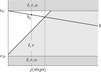
Since our path is eqlevel-decreasing (the eqlevel drops by $1$ in each step), we know that $b_{j}=e_{U}-j$, which is depicted by a line (in the standard sense, having nothing to do with IL-equality lines) starting in point $(0,e_{U})$ and having the slope $-1$. (For a better overall appearence, the vertical unit length in Fig. 10 is smaller than the horizontal one.)

Each $o_{j}$ is either $\omega$ or an element of ZE (of $\textsc{E}_{3}$ after Def. 12); in particular, $o_{j}\geq e_{U}$ or $o_{j}\leq e_{D}$, which is depicted as a constraint in Fig. 10, using the horizontal lines at levels $e_{U}$ and $e_{D}$.

We now recall Prop. 16 and the fact that each finite $\mathsf{IL}(q(0))$ is in ZE (in $\textsc{E}_{2}$ after Def. 12). Hence for each $\ell_{j}$ we have either $\ell_{j}\geq e_{U}$ or $\ell_{j}\leq e_{D}+\rho_{\textsc{m}}\cdot j+\sigma_{\textsc{m}}$ where $\rho_{\textsc{m}}$ is the maximal number appearing as $\rho$ in the fixed equalities $\mathsf{IL}(p(m))=\rho\cdot m+\sigma+e$, and $\sigma_{\textsc{m}}$ is the maximal number appearing there as $\sigma$. (We use the fact that the counter value is at most $j$ in $C_{j}$, as well as in $C^{\prime}_{j}$ when $C^{\prime}_{j}$ is also in $\mathcal{T}(\mathcal{A})$, since we started from zero configurations.) We recall that both $\rho_{\textsc{m}}$ and $\sigma_{\textsc{m}}$ are small rational numbers. The above constraints on $\ell_{j}$ are also depicted in Fig. 10, using the horizontal line at level $e_{U}$ and the line starting in $(0,e_{D}{+}\sigma_{\textsc{m}})$ and having the slope $\rho_{\textsc{m}}$. The same constraints hold for $r_{j}$.

We note that if the horizontal coordinate of the intersection of the “$b$-line” (with slope ${-}1$) and the “$\ell,r$-line” (with the slope $\rho_{\textsc{m}}$) is small then $e_{U}-e_{D}$ is small. This is clear by noting that $b_{j}=e_{U}{-}j\leq e_{D}+\rho_{\textsc{m}}\cdot j+\sigma_{\textsc{m}}$ implies $e_{U}{-}e_{D}\leq(1{+}\rho_{\textsc{m}})\cdot j+\sigma_{\textsc{m}}$.

In fact, we will show even something stronger, namely that the maximal prefix of our path in which $b_{j}$ (for $j>0$) is “solitary”, i.e. $b_{j}\not\in\{\ell_{j},r_{j},o_{j}\}$, is short. This will be based on Cor. 20, applied to the “rectangle” $(b_{j},\ell_{j},r_{j},o_{j})$. The previously established facts, like that about few possible values $o_{j}$, will entail that in a long b-solitary prefix we would “usually” have $\ell_{j}=r_{j}<\omega$, which in turn would entail a long line-climbing segment; this would contradict Prop. 29.

Definition 30.

A pair $(C,C^{\prime})$ of stable configurations in $\mathcal{T}_{\mathsf{ext}}(\mathcal{A})$ with the associated eqlevel tuple $(b,\ell,r,o,d^{L},d^{R})$ is b-solitary if $b\not\in\{\ell,r,o\}$.
A path in $\mathcal{T}_{\mathsf{ext}}(\mathcal{A})\times\mathcal{T}_{\mathsf{ext}}(\mathcal{A})$ is b-solitary if each configuration-pair in the path is b-solitary.

We note that in a b-solitary pair $(C,C^{\prime})$ we must have that at least $C$ is in $\mathcal{T}(\mathcal{A})$, by our choice in Def. 18.

Lemma 31.

All gaps $e_{U}{-}e_{D}$ in ZE are small.

Proof.

We assume some $e_{D},e_{U}\in\textsc{ZE}$ where $e_{D}<e_{U}$ and there is no $e\in\textsc{ZE}$ such that $e_{D}<e<e_{U}$, and consider an eqlevel-decreasing path

$$(C_{0},C^{\prime}_{0})\stackrel{{\scriptstyle a_{1}}}{{\longrightarrow}}(C_{1},C^{\prime}_{1})\stackrel{{\scriptstyle a_{2}}}{{\longrightarrow}}(C_{2},C^{\prime}_{2})\stackrel{{\scriptstyle a_{3}}}{{\longrightarrow}}\cdots\stackrel{{\scriptstyle a_{z}}}{{\longrightarrow}}(C_{z},C^{\prime}_{z})$$ (9)

in $\mathcal{T}_{\mathsf{ext}}(\mathcal{A})\times\mathcal{T}_{\mathsf{ext}}(\mathcal{A})$ where $C_{0},C^{\prime}_{0}$ are stable zero configurations, $C_{0}\stackrel{{\scriptstyle e_{U}}}{{\longleftrightarrow}}C^{\prime}_{0}$, and $C_{z}\stackrel{{\scriptstyle 0}}{{\longleftrightarrow}}C^{\prime}_{z}$. We thus have $\mathsf{EqL}(C_{j},C^{\prime}_{j})=e_{U}-j$ for all $j\in\{0,1,\dots,z\}$.

Our aim is to show that $e_{U}-e_{D}$ is small. If $C_{0}\in Q_{\mathsf{Mod}}$ and $C^{\prime}_{0}\in Q_{\mathsf{Mod}}$ then $C_{1},C^{\prime}_{1}$ are also (stable) zero configurations, and thus $\mathsf{EqL}(C_{1},C^{\prime}_{1})=e_{U}{-}1\in\textsc{ZE}$; we thus have $e_{U}-e_{D}=1$.

We thus further assume that $C_{0}\not\in Q_{\mathsf{Mod}}$ (while $C^{\prime}_{0}\not\in Q_{\mathsf{Mod}}$ is handled by symmetry). Let $(b_{i},\ell_{i},r_{i},o_{i},d^{L}_{i},d^{R}_{i})$ be the eqlevel tuple associated with $(C_{i},C^{\prime}_{i})$ ($i=0,1,\dots,z$), as in Def. 18; in the case $C^{\prime}_{i}\in Q_{\mathsf{Mod}}$ we thus have $r_{i}=\omega$, $b_{i}=d^{L}_{i}$, $o_{i}=d^{R}_{i}$.

We now note that if there is some small $j>0$ such that $(C_{j},C^{\prime}_{j})$ is not b-solitary then $e_{U}-e_{D}$ is small. This follows from the following two facts.

1. If $b_{j}=o_{j}$ then $b_{j}=e_{U}-j\leq e_{D}$ (since $o_{i}$ belongs to ZE for all $i$); hence $e_{U}-e_{D}\leq j$.

2. If $b_{j}=\ell_{j}$ or $b_{j}=r_{j}$ then $b_{j}=e_{U}-j\leq e_{D}+\rho_{\textsc{m}}\cdot j+\sigma_{\textsc{m}}$, and thus $e_{U}{-}e_{D}\leq(1{+}\rho_{\textsc{m}})\cdot j+\sigma_{\textsc{m}}$, as was already discussed before Def. 30.

We now fix $j$ so that

$$(C_{1},C^{\prime}_{1})\stackrel{{\scriptstyle a_{2}}}{{\longrightarrow}}(C_{2},C^{\prime}_{2})\stackrel{{\scriptstyle a_{3}}}{{\longrightarrow}}\cdots\stackrel{{\scriptstyle a_{j}}}{{\longrightarrow}}(C_{j},C^{\prime}_{j})$$ (10)

is the maximal b-solitary prefix of the path (9) in which the first step is removed. We will show that $j$ is small, by which the proof will be finished; we further assume $j\geq 1$.

The assumption $C_{0}\not\in Q_{\mathsf{Mod}}$ implies $C_{1}\not\in Q_{\mathsf{Mod}}$ (hence $C_{1}=p(m)$ for some $p\in Q_{\mathsf{St}}$ and some $m\in\{0,1\}$). Suppose $(C_{1},C^{\prime}_{1})\stackrel{{\scriptstyle a_{2}}}{{\longrightarrow}}(C_{2},C^{\prime}_{2})\stackrel{{\scriptstyle a_{3}}}{{\longrightarrow}}\cdots\stackrel{{\scriptstyle a_{j_{1}}}}{{\longrightarrow}}(C_{j_{1}},C^{\prime}_{j_{1}})$ is the maximal prefix of (10) such that $C^{\prime}_{j_{1}}\in Q_{\mathsf{Mod}}$; we put $j_{1}=0$ if $C^{\prime}_{1}\not\in Q_{\mathsf{Mod}}$. For all $i\in\{1,2,\dots j_{1}\}$ we have $b_{i}=e_{U}-i$, $r_{i}=\omega$, and $b_{i}\not\in\{\ell_{i},r_{i},o_{i}\}$; hence $\ell_{i}=o_{i}<b_{i}$ (by Cor. 20). By Prop. 10(2) and Prop. 17(1), the set $\{C_{i}\mid 1\leq i\leq j_{1}\}$ is small, which implies that the set $\{b_{i}\mid 1\leq i\leq j_{1}\}=\{d^{L}_{i}\mid 1\leq i\leq j_{1}\}$ is small, by Prop. 11(2). Since $b_{i_{1}}\neq b_{i_{2}}$ if $i_{1}\neq i_{2}$, we get that $j_{1}$ is small. It is thus sufficient to show that the suffix

$$(C_{j_{1}+1},C^{\prime}_{j_{1}+1})\stackrel{{\scriptstyle a_{j_{1}+2}}}{{\longrightarrow}}(C_{j_{1}+2},C^{\prime}_{j_{1}+2})\stackrel{{\scriptstyle a_{j_{1}+3}}}{{\longrightarrow}}\cdots\stackrel{{\scriptstyle a_{j}}}{{\longrightarrow}}(C_{j},C^{\prime}_{j})$$ (11)

of (10) is short. Let us rewrite (11) as

$$(p_{0}(m_{0}),q_{0}(n_{0}))\stackrel{{\scriptstyle a^{\prime}_{1}}}{{\longrightarrow}}(p_{1}(m_{1}),q_{1}(n_{1}))\stackrel{{\scriptstyle a^{\prime}_{2}}}{{\longrightarrow}}\cdots\stackrel{{\scriptstyle a^{\prime}_{j^{\prime}}}}{{\longrightarrow}}(p_{j^{\prime}}(m_{j^{\prime}}),q_{j^{\prime}}(n_{j^{\prime}}))$$ (12)

where $j^{\prime}=j-(j_{1}{+}1)$, and $(p_{i}(m_{i}),q_{i}(n_{i}))=(C_{j_{1}+1+i},C^{\prime}_{j_{1}+1+i})$, $a^{\prime}_{i}=a_{j_{1}+1+i}$ for $i=0,1,\dots,j^{\prime}$. We note that $m_{0}+n_{0}$ is small (since $j_{1}$ is small and $C_{0},C^{\prime}_{0}$ are zero configurations).

For simplicity, by $(b_{i},\ell_{i},r_{i},o_{i},d^{L}_{i},d^{R}_{i})$, where $0\leq i\leq j^{\prime}$, we further denote the eqlevel tuple associated with $(p_{i}(m_{i}),q_{i}(n_{i}))$ (not with $(C_{i},C^{\prime}_{i})$ anymore). Since the path (12) is eqlevel-decreasing, there is no repeat, i.e. $(p_{i_{1}}(m_{i_{1}}),(q_{i_{1}}(n_{i_{1}}))\neq(p_{i_{2}}(m_{i_{2}}),(q_{i_{2}}(n_{i_{2}}))$ if $i_{1}\neq i_{2}$.

For each $i\in\{0,1,\dots,j^{\prime}\}$, the pair $(p_{i}(m_{i}),q_{i}(n_{i}))$ is b-solitary, and thus

$\min\{b_{i},\ell_{i},r_{i},o_{i}\}$ is $r_{i}=o_{i}$ or $\ell_{i}=o_{i}$ or $\ell_{i}=r_{i}$.

We now aim to show that

$$\text{there are only few }i\in\{0,1,\dots,j^{\prime}\}\text{ for which we do not have }\ell_{i}=r_{i}<\omega.$$ (13)

To establish (13), it suffices to show that the sets $\{i\mid 0\leq i\leq j^{\prime},r_{i}=o_{i}<\omega\}$ and $\{i\mid 0\leq i\leq j^{\prime},\ell_{i}=o_{i}<\omega\}$ are small; by symmetry it suffices just to show that the former set is small.

We first note that the set

$$\{q_{i}(n_{i})\mid 0\leq i\leq j^{\prime},r_{i}=o_{i}<\omega\}$$

is small by Prop. 10(2) and 17(1). Hence also the set

$$\{d^{R}_{i}\mid 0\leq i\leq j^{\prime},r_{i}=o_{i}<\omega\}$$

is small, by Prop. 11(2). The set

$$\{i\mid 0\leq i\leq j^{\prime},r_{i}=o_{i}<\omega,\min\{b_{i},\ell_{i},d^{R}_{i}\}=b_{i}=d^{R}_{i}\}$$

is thus also small (recall that $b_{i_{1}}\neq b_{i_{2}}$ if $i_{1}\neq i_{2}$). The set

$$\{p_{i}(m_{i})\mid 0\leq i\leq j^{\prime},r_{i}=o_{i}<\omega,\min\{b_{i},\ell_{i},d^{R}_{i}\}=\ell_{i}=d^{R}_{i}\}$$

is also small, by recalling Prop. 17(1). Since $\min\{b_{i},\ell_{i},d^{R}_{i}\}$ is $\ell_{i}=d^{R}_{i}$ or $b_{i}=d^{R}_{i}$ for all $i\in\{0,1\dots,j^{\prime}\}$ (recall that $b_{i}=\ell_{i}$ is excluded in b-solitary pairs), we get that both sets

$\{q_{i}(n_{i})\mid 0\leq i\leq j^{\prime},r_{i}=o_{i}<\omega\}$ and $\{p_{i}(m_{i})\mid 0\leq i\leq j^{\prime},r_{i}=o_{i}<\omega\}$

are small. Since there is no repeat in (12), we get that the set $\{i\mid 0\leq i\leq j^{\prime},r_{i}=o_{i}<\omega\}$ is small. We have thus established (13).

Let us now consider the sum-increasing subsequence

$$(p_{i_{0}}(m_{i_{0}}),q_{i_{0}}(n_{i_{0}})),(p_{i_{1}}(m_{i_{1}}),q_{i_{1}}(n_{i_{1}})),(p_{i_{2}}(m_{i_{2}}),q_{i_{2}}(n_{i_{2}})),\dots$$ (14)

of the sequence of pairs in (12), where $0=i_{0}<i_{1}<i_{2}<\cdots$, and $i_{h+1}$ is the first such that $m_{i_{h+1}}+n_{i_{h+1}}$ is bigger than $m_{i_{h}}+n_{i_{h}}$ (for $h=0,1,2,\dots$). If this subsequence is short then (12) is obviously short since we started with small $m_{0}+n_{0}$ and $m_{i_{h+1}}+n_{i_{h+1}}\leq m_{i_{h}}+n_{i_{h}}+2$ (and there is no repeat in (12)).

For $h=0,1,2\dots$ we now consider the subpaths of (12) starting in $(p_{i_{h}}(m_{i_{h}}),q_{i_{h}}(n_{i_{h}}))$ and finishing in $(p_{i_{h+1}}(m_{i_{h+1}}),q_{i_{h+1}}(n_{i_{h+1}}))$; we call them segments. A segment is called unusual if

• the segment visits a pair $(p(m),q(n))$ such that $(m,n)$ is in no line-bunch, or is in the intersection of two different line-bunches, or satisfies $m=0$ or $n=0$, or

• the segment contains a step $(p(m),q(n))\stackrel{{\scriptstyle a}}{{\longrightarrow}}(p^{\prime}(m{+}j_{1}),q^{\prime}(n{+}j_{2}))$ such that $(m,n)$ and $(m{+}j_{1},n{+}j_{2})$ are in two different line-bunches.

Using (13) and Prop. 25 and the no-repeat property, we can easily verify that there are only few unusual segments.

Any other segment, called usual, is thus a positive path projected to one line-bunch; moreover, the concatenation of consecutive usual segments is also projected to one line-bunch. We note that if $(p_{i_{h}}(m_{i_{h}}),q_{i_{h}}(n_{i_{h}}))$ and $(p_{i_{h^{\prime}}}(m_{i_{h^{\prime}}}),q_{i_{h^{\prime}}}(n_{i_{h^{\prime}}}))$, for $h<h^{\prime}$, are in the same line then $m_{i_{h}}<m_{i_{h^{\prime}}}$. Since there are only few lines, less than some small $\mathsf{b}_{1}$, and the lengths of eqlevel-decreasing line-climbing paths are less than some small $\mathsf{b}_{2}$ by Prop. 29, we cannot have more than $\mathsf{b}_{1}\cdot\mathsf{b}_{2}$ consecutive usual segments. This finally implies that (14) is short, and thus also (12) is short. Hence $e_{U}-e_{D}$ is small. ∎

Now Lemma 13 and Lemma 31 give a proof of Theorem 14, and thus also of Theorem 2.

4 Additional remarks

The notions and their properties from the main proof also help to answer related questions. Here we only mention regularity. It is straightforward to verify that the language (the set of enabled traces) of a doca configuration $p(m)$ is non-regular iff we have $p(m)\stackrel{{\scriptstyle u}}{{\longrightarrow}}q_{1}(n)\stackrel{{\scriptstyle v}}{{\longrightarrow}}q_{2}(n{+}k)\stackrel{{\scriptstyle w}}{{\longrightarrow}}q^{\prime}(0)$ where $q_{1}(n)\stackrel{{\scriptstyle vw}}{{\longrightarrow}}q^{\prime}(0)$ is a positive path and $\mathsf{IL}(q^{\prime}(0))<\omega$. (In this case, from $p(m)$ we can reach $q(n^{\prime}))$ for some $q$ and infinitely many $n^{\prime}$ where $\mathsf{IL}(q(n^{\prime}))<\omega$.) It is then a routine (though a bit technical) to show that the regularity problem for doca is in $\mathsf{NL}$ (and $\mathsf{NL}$-complete) as well.

Appendix (classical doca equivalence)

Figure 11: A classical doca

The aim of this Appendix is to sketch the ideas of a routine reduction of the standard doca language equivalence problem to our Doca-Eq. A classical definition would define a doca as a tuple $\mathcal{A}=(Q,\Sigma,\delta,q_{0},F)$ where $Q$ is a finite set of control states, $\Sigma$ is a finite alphabet, $\delta\subseteq Q\times(\Sigma\cup\{\varepsilon\})\times\{0,1\}\times Q\times\{-1,0,1\}$ is a transition relation satisfying the below given two conditions, $q_{0}\in Q$ is the initial state, and $F\subseteq Q$ is the set of accepting states.

In this context, $\varepsilon\not\in\Sigma$ is handled as a special symbol but it plays the role of the empty word in the semantics. The conditions for $\delta$ are the following.

1. For each triple $(p,a,c)$, where $p\in Q$, $a\in\Sigma\cup\{\varepsilon\}$, $c\in\{0,1\}$ there is at most one pair $(q,j)$ such that $(p,a,c,q,j)\in\delta$; moreover, $j\neq-1$ if $c=0$.

2. If $(p,\varepsilon,c,q,j)\in\delta$ then there are no $a\in\Sigma$, $q^{\prime}\in Q$, $j^{\prime}\in\{-1,0,1\}$ such that $(p,a,c,q^{\prime},j^{\prime})\in\delta$.

A configuration of $\mathcal{A}$ is a pair $(p,n)\in Q\times\mathbb{N}$; we write $p(n)$ instead of $(p,n)$, as previously. We now define relations $\stackrel{{\scriptstyle w}}{{\longrightarrow}}$, $w\in\Sigma^{*}$, on $Q\times\mathbb{N}$ inductively as follows: $p(n)\stackrel{{\scriptstyle\varepsilon}}{{\longrightarrow}}p(n)$; if $(p,a,\text{sgn}(n),q,j)\in\delta$ (where $a\in\Sigma\cup\{\varepsilon\}$) then $p(n)\stackrel{{\scriptstyle a}}{{\longrightarrow}}q(n{+}j)$ (here $\text{sgn}(n)=1$ if $n>0$ and $\text{sgn}(n)=0$ if $n=0$); if $p(n)\stackrel{{\scriptstyle u}}{{\longrightarrow}}p^{\prime}(n^{\prime})$ and $p^{\prime}(n^{\prime})\stackrel{{\scriptstyle v}}{{\longrightarrow}}p^{\prime\prime}(n^{\prime\prime})$ then $p(n)\stackrel{{\scriptstyle uv}}{{\longrightarrow}}p^{\prime\prime}(n^{\prime\prime})$. Since the symbol $\varepsilon$ is handled as the empty word, we have $\varepsilon u=u\varepsilon=u$. We define the language accepted by $\mathcal{A}$ as

$L(\mathcal{A})=\{w\in\Sigma^{*}\mid q_{0}(0)\stackrel{{\scriptstyle w}}{{\longrightarrow}}q(n)$ for some $q\in F$, $n\in\mathbb{N}\}$.

The language equivalence problem asks, given two doca $\mathcal{A}_{1}$, $\mathcal{A}_{2}$ if $L(A_{1})=L(A_{2})$.

We now sketch the ideas of reducing this problem to our problem Doca-Eq. First we note that we can take the disjoint union $\mathcal{A}$ of $\mathcal{A}_{1},\mathcal{A}_{2}$ and ask about the equality of languages of two different (initial) configurations. The doca $\mathcal{A}$, with $k$ control states, can be routinely replaced by a doca $\mathcal{A}_{\mathsf{SC}}$ (with the “Shrinked Counter”), where a configuration $p(m)$ of $\mathcal{A}$ is represented by the configuration $p_{i}(j)$ of $\mathcal{A}_{\mathsf{SC}}$ where $i=m\bmod k$ and $j=(m\div k)$. The control state set of $\mathcal{A}_{\mathsf{SC}}$ is $k$-times bigger, to pay for shrinking the counter.

It is then easy to get rid of $\varepsilon$-rules which are not in $\varepsilon$-cycles, and to get rid of $\varepsilon$-cycles with nonnegative effects. Finally, the only $\varepsilon$-rules which remain are popping (decrementing the counter), and they are in cycles, which is exemplified by the states $s_{1},s_{2},s_{3}$ in Fig. 11. To each such state $s$ in an $\varepsilon$-cycle we can add a control state $q_{s}$ with the zero rule $(s,\varepsilon,0,q_{s},0)$, to clearly separate the “reset control states” from the “stable ones”; this is illustrated by $q^{\prime}_{1},q^{\prime}_{2},q^{\prime}_{3}$ in Fig. 11. The final step of the transformation to our reset-form doca (as in Fig. 1) is now obvious. In the example, all $s_{1},s_{2},s_{3}$ get the period $3$, and we put $\mathsf{goto}_{s_{2}}(2)=q^{\prime}_{1}$, $\mathsf{goto}_{s_{3}}(0)=q^{\prime}_{3}$, etc. (In fact, using $s_{1}$ is sufficient in our special case since the non-$\varepsilon$ incoming arcs of $s_{2},s_{3}$ correspond to zero rules only.)

Trace equivalence coincides with language equivalence when all states are declared as accepting. A reduction from language equivalence to trace equivalence can be sketched as follows. For any triple $(q,a,c)$ such that $q\in Q_{\mathsf{St}}$, $a\in\Sigma$, $c\in\{0,1\}$ and there is no $(q,a,c,q^{\prime},j)\in\delta$ we add the rule $(q,a,c,q_{\mathsf{sink}},0)$ where $q_{\mathsf{sink}}$ is an added “sink loop” state, with rules $(q_{\mathsf{sink}},a,c,q_{\mathsf{sink}},0)$ for all $a\in\Sigma$ and $c\in\{0,1\}$. We assume having arranged that all accepting control states are stable, and we now add the “loop” rules $(q,a_{\mathsf{acc}},c,q,0)$ for a special fresh letter $a_{\mathsf{acc}}$ and all $q\in F$, $c\in\{0,1\}$ (so that $\mathsf{EqL}(p(m),q(n))=0$ when $p\in F$, $q\not\in F$ or vice versa).

Since the reduction keeps the lengths of non-equivalence witnesses polynomially related, the analogues of Theorems 2 and 3 hold for the classical equivalence problem as well.

References

- [1] P. Berman and R. Roos. Learning One-Counter Languages in Polynomial Time (Extended Abstract). In Proc. of FOCS, pages 61–67. IEEE, 1987.
- [2] S. Böhm and S. Göller. Language Equivalence of Deterministic Real-Time One-Counter Automata Is NL-Complete. In MFCS, volume 6907 of Lecture Notes in Computer Science, pages 194–205. Springer, 2011.
- [3] S. Böhm, S. Göller, and P. Jančar. Bisimilarity of one-counter processes is PSPACE-complete. In Proc. of CONCUR, volume 6269 of Lecture Notes in Computer Science, pages 177–191. Springer, 2010.
- [4] W. Czerwiński and S. Lasota. Fast equivalence-checking for normed context-free processes. In Proc. FSTTCS’10, volume 8 of LIPIcs. Schloss Dagstuhl - Leibniz-Zentrum fuer Informatik, 2010.
- [5] A. F. Fahmy and R. S. Roos. Efficient Learning of Real Time One-Counter Automata. In Proc. of ALT, volume 997 of Lecture Notes in Computer Science, pages 25–40. Springer, 1995.
- [6] S. Göller, C. Haase, J. Ouaknine, and J. Worrell. Model Checking Succinct and Parametric One-Counter Automata. In Proc. of ICALP (2), volume 6199 of Lecture Notes in Computer Science, pages 575–586. Springer, 2010.
- [7] S. Göller and M. Lohrey. Branching-time model checking of one-counter processes. In Proc. of STACS, volume 5 of LIPIcs, pages 405–416. Schloss Dagstuhl - Leibniz-Zentrum fuer Informatik, 2010.
- [8] S. Göller, R. Mayr, and A. W. To. On the computational complexity of verifying one-counter processes. In Proc. of LICS, pages 235–244. IEEE Computer Society Press, 2009.
- [9] C. Haase, S. Kreutzer, J. Ouaknine, and J. Worrell. Reachability in succinct and parametric one-counter automata. In Proc. of CONCUR, volume 5710 of Lecture Notes in Computer Science, pages 369–383. Springer, 2009.
- [10] K. Higuchi, M. Wakatsuki, and E. Tomita. A polynomial-time algorithm for checking the inclusion for real-time deterministic restricted one-counter automata which accept by final state. IEICE Trans. Information and Systems, E78-D:939–950, 1995.
- [11] K. Higuchi, M. Wakatsuki, and E. Tomita. A polynomial-time algorithm for checking the inclusion for real-time deterministic restricted one-counter automata which accept by accept mode. IEICE Trans. Information and Systems, E81-D:1–11, 1998.
- [12] Y. Hirshfeld, M. Jerrum, and F. Moller. A Polynomial Algorithm for Deciding Bisimilarity of Normed Context-Free Processes. Theor. Comput. Sci., 158(1&2):143–159, 1996.
- [13] P. Jančar. Decidability of dpda language equivalence via first-order grammars. In LICS, pages 415–424. IEEE, 2012.
- [14] P. Jančar, A. Kučera, and F. Moller. Simulation and bisimulation over one-counter processes. In Proc. of STACS, volume 1770 of Lecture Notes in Computer Science, pages 334–345, 2000.
- [15] P. Jančar, F. Moller, and Z. Sawa. Simulation Problems for One-Counter Machines. In Proc. of SOFSEM, volume 1725 of Lecture Notes in Computer Science, pages 404–413. Springer, 1999.
- [16] R. Mayr. Undecidability of Weak Bisimulation Equivalence for 1-Counter Processes. In Proc. of ICALP, volume 2719 of Lecture Notes in Computer Science, pages 570–583, 2003.
- [17] M. Oyamaguchi. The equivalence problem for real-time DPDAs. J. ACM, 34:731–760, 1987.
- [18] R. Roos. Deciding Equivalence of Deterministic One-Counter Automata in Polynomial Time with Applications to Learning. PhD thesis, The Pennsylvania State University, 1988.
- [19] G. Sénizergues. L(A)=L(B)? decidability results from complete formal systems. Theor. Comput. Sci., 251(1-2):1–166, 2001.
- [20] G. Sénizergues. L(A)=L(B)? A simplified decidability proof. Theor. Comput. Sci., 281(1-2):555–608, 2002.
- [21] G. Sénizergues. The Equivalence Problem for t-Turn DPDA Is Co-NP. In Proc. of ICALP, volume 2719 of Lecture Notes in Computer Science, pages 478–489. Springer, 2003.
- [22] C. Stirling. Deciding DPDA Equivalence Is Primitive Recursive. In Proc. of ICALP, volume 2380 of Lecture Notes in Computer Science, pages 821–832. Springer, 2002.
- [23] L. G. Valiant and M. Paterson. Deterministic one-counter automata. J. Comput. Syst. Sci., 10(3):340–350, 1975.