Universality Classes in Constrained Crack Growth

Abstract

Based on an extension of the fiber bundle model we investigate numerically the motion of the crack front through a weak plane separating a soft and an infinitely stiff block. We find that there are two regimes. At large scales the motion is consistent with the pinned elastic line model and we find a roughness exponent equal to $0.39\pm 0.04$ characterizing it. At smaller scales, coalescence of holes dominates the motion rather than pinning of the crack front. We find a roughness exponent consistent with 2/3, which is the gradient percolation value. The length of the crack front is fractal on these smaller scales. We determine its fractal dimension to be $1.77\pm 0.02$, consistent with the hull of percolation clusters, 7/4. This suggests that the crack front is described by two universality classes: on large scales, the pinned elastic line one and on small scales, the percolation universality class.

Schmittbuhl and Måløy sm97 were the first to study experimentally the roughness of a crack front moving along a weak plane in a material loaded under mode I conditions. By sintering two sandblasted plexiglass plates together and then plying them apart from one edge, they were able to follow the motion of the crack front moving along the sintered boundary between the two plates. The rough crack front turned out to be self affine, i.e., its height-height correlation function $\langle(h(x+\Delta x)-h(x))^{2}\rangle$ scaled as $|\Delta x|^{\zeta}$ where $\zeta$ is the rougness exponent. $h(x)$ is the position of the crack front with respect to a base line orthogonal to the average crack growth direction and $x$ is the coordinate along this base line. The roughness exponent was found to be $\zeta=0.55\pm 0.05$. A couple of years before this work, Schmittbuhl et al. srvm95 studied numerically a model of such constrained crack growth based on regarding the motion of the crack front as that of a pinned elastic line, the fluctuating line model. This work was based on an earlier idea by Bouchaud et al. bblp93 . The conclusion of Schmittbuhl et al. was that the front should be rough and self affine, characterized by a roughness exponent $\zeta=0.35\pm 0.05$. This value was later refined to $0.388\pm 0.002$ by Rosso and Krauth rk02 . The large discrepancy between the numerical and experimental results — the latter having been refined to $\zeta=0.63\pm 0.03$ by improving the statistical analysis dsm99 — spurred a lively quest for an explanation that only today seems to converge towards a satisfactory understanding of the underlying physics , see e.g. b09 ; bb11 for a review.

An attempt at finding an explanation for the large roughness exponent seen in the experiments that was not based on some variation on the fluctuating line model was forwarded by Schmittbuhl et al. shb03 . The underlying idea here was that the crack front did not advance due to a competition between effective elastic forces and pinning forces at the front, but by coalescence of damage in front of the crack with the advancing crack itself. Such an idea had been put forwards in a more general context by Bouchaud et al. bbfrr02 the year before. By using a grid of linearly elastic fibers connected to a soft elastic half space, Schmittbuhl et al. found a rougness exponent of $\zeta=0.60\pm 0.05$, which was consistent with the experimental results. The crack advance mechanism in this model was analyzed in terms of a correlated gradient percolation process where coalescence is the dominating mechanism.

Recently, Santucci et al. sgtshm10 reanalyzed data from a number of earlier studies, including dsm99 , finding that the crack front has two scaling regimes: one small-scale regime described by a roughness exponent $\zeta_{-}=0.60\pm 0.05$ and a large-scale regime described by a roughness exponent $\zeta_{+}=0.35\pm 0.05$.

We suggest in this letter that there are indeed two competing mechanisms involved in generating the scaling properties seen in the roughness of the crack front: on small scales coalescence dominates, whereas on large scales, the fluctuating line picture is correct. There is a crossover between the regimes where either of the two mechanisms dominate associated with a well-defined crossover length scale.

Our numerical work strongly suggest that the coalescence mechanism seen at small scales is controlled by the ordinary percolation critical point, leading to percolation exponents. This is in constrast to Schmittbuhl et al. shb03 who suggested a new percolation-like universality class, but consistent with recent theoretical work on fracture in the fuse model szs12 .

We note an earlier attempt at explaining the two scaling regimes seen in Ref. sgtshm10 based solely on the fluctuating line model lsz10 . Here Laurson et al. lsz10 relate the crossover to the Larkin length scale of the crack front lo79 . This is in this context the length scale at which the roughness of the front is comparable to the correlation length inherent to the pinning disorder.

Our numerical system is a fiber bundle model phc10 closely related to the one used in shb03 and introduced by Batrouni et al. the year before bhs02 . $L\times L$ elastic fibers are placed in a square lattice between two clamps. One of the clamps is infinely stiff whereas the other has a finite Young modulus $E$ and a Poisson ratio $\nu$. All fibers are equally long and have the same elastic constant $k$. We measure the position of the stiff clamp with respect its position when all fibers carry zero force, $D$. The force carried by the fiber at position $(i,j)$, where $i$ and $j$ are coordinates in a cartesian coordinate system oriented along the edges of the system, is then

$$f_{(i,j)}=-k(u_{(i,j)}-D)\;,$$ (1)

where $u_{(i,j)}$ is the fiber’s elongation. The fibers redistribute the forces they carry through the response of the clamp with finite elastisity. The redistribution of forces is accomplished by using the Green function connecting the force $f_{(m,n)}$ acting on the clamp from fiber $(m,n)$ with the deformation $u_{(i,j)}$ at fiber $(i,j)$, j85

$$u_{(i,j)} =\sum_{(m,n)}G_{(i,j),(m,n)}f_{(m,n)},$$ (2a)

$$G_{(i,j),(m,n)} =$$

$$\frac{1-\nu^{2}}{\pi Ea^{2}} \int^{a/2}_{-a/2}dx\ \int^{a/2}_{-a/2}dy\ \frac{1}{|\vec{r}_{(i,j)}-\vec{r}_{(m+x,n+y)}|}.$$ (2b)

where $a$ is the distance between neighboring fibers. $\vec{r}_{(i,j)}-\vec{r}_{(m,n)}$ is the distance between fibers $(i,j)$ and $(m,n)$ and the integration runs over the $a\times a$ square around fiber $(m,n)$. This equation set is solved using a Fourier accelerated conjugate gradient method bhn86 ; bh88 .

Figure 1: Parts of the crack fronts obtained in the simulations. The color black represents broken bonds and white represents unbroken bonds. To the left, a) is an example from a system with a high rescaled Young modulus $e$ being driven forwards (upwards) primarily by coalescence with damage forming ahead of the crack front. (b) is an example from a system with a low $e$. This system is being driven forward by damage forming on the crack front. Small $e=2\times 10^{-3}$ is equivalent to a larger system than one with a large $e=0.8$.

We note that the Green function, Eq. (2b), is proportional to $(Ea)^{-1}$. The elastic constant of the fibers, $k$, must be proportional to $a^{2}$. The linear size of the system is $aL$. Hence, by changing the linear size of the system without changing the discretization $a$, we change $L\to\lambda L$ but leave $(Ea)$ and $k$ unchanged. If we on the other hand change the discretization without changing the linear size of the system, we simultaneously set $L\to\lambda L$, $(Ea)\to\lambda(Ea)$ and $k\to k/\lambda^{2}$. We define the scaled Young modulus $e=(Ea)/L$. Hence, changing $e$ without changing $k$ is equivalent to changing $L$ — and hence the linear size of the system — while keeping the elastic properties of the system constant sgh12 .

Bonds are broken by using the quasistatic approach h05 . That is, we assign to each fiber $(i,j)$ a threshold value $t_{(i,j)}$. Bonds are broken one by one by each time identifying $\max_{(i,j)}(f_{(i,j)}/t_{(i,j)})$ for $D=1$. This ratio is then used to read off the value $D$ at which the next fiber breaks.

In the constrained crack growth experiments of Schmittbuhl and Måløy sm97 , the two sintered plexiglass plates were plied apart from one edge. In the numerical modeling of Schmittbuhl et al. shb03 , an asymmetric loading was accomplished by introducing a linear gradient in $D$. Rather than implementing an asymmetric loading, we introduce a gradient in the threshold distribution, $t_{(i,j)}=gj+r_{(i,j)}$, where $g$ is the gradient and $r_{(i,j)}$ is a random number drawn from a flat distribution on the unit interval. In the limit of large Young modulus $E$, this system becomes equivalent to the gradient percolation problem srg85 ; gr05 .

In order to follow the crack front as the breakdown process develops, we implement the “conveyor belt” technique drp01 ; gsh12 where a new upper row of intact fibers is added and a lower row of broken fibers removed from the system at regular intervals. This makes it possible to follow the advancing crack front indefinitely. The implementation has been described in detail in gsh12 .

Figure 2: Averaged wavelet coefficient $W(a)$ based on transforming $h_{i}$ vs. $a$ for $e=7.8125\times 10^{-4}$, $L=256$ ($g=0.00625$, averaged over 4200 fronts) and $L=512$ ($g=0.003125$, averaged over 850 fronts). The slope of the straight line is $0.39+1/2$.

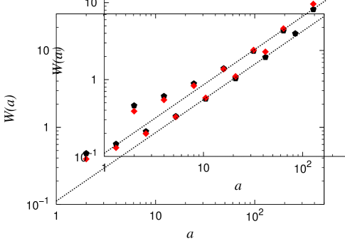
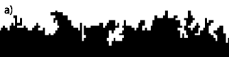
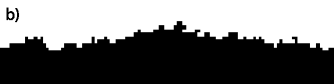
Figure 1 shows two examples of typical crack fronts representative of a stiff (high $e=0.8$) and a soft system (low $e=2\times 10^{-3}$). In both cases, the front is viewed from above (and propagation corresponds to an upwards movement in the figure). The two fronts are quite different. Even though we change the Young modulus $E$ between the two crack fronts, this is equivalent to changing the scale at which the fronts are viewed: Small $e$ corresponds to a large scale and vice versa.

We identify the crack front by first eliminating all islands of surviving fibers behind it and all islands of failed fibers in front of it. We measure “time” $n$ in terms of the number of failed fibers. After an initial period, the system settles into a steady state. We then record the position of the crack front $j=j(i,n=0)$ after having set $n=0$. We then define the position at later times $n>0$ relative to this initial position,

$$h_{i}(n)=j(i,n)-j(i,n=0)\;.$$ (3)

This is the same definition as was used by Schmittbuhl and Måløy sm97 . The front as it has now been defined will contain overhangs. That is, there may be multiple values of $h_{i}(n)$ for the same $i$ and $n$ values. We only keep the largest $h_{i}(n)$, i.e. we implement the Solid-on-Solid (SOS) front.

We define the average position of the front as $\langle h(n)\rangle=\sum_{i=1}^{L}h_{i}(n)/L$ and the front width as $w(n)^{2}=\sum_{i=1}^{L}(h_{i}(n)-\langle h(n)\rangle)^{2}/L$.

We will in the following explore the model going from large to small values of the Young modulus $E$ while keeping $k$ fixed. As already discussed, this is equivalent to changing the system size $L$ while keeping $E$ fixed.

Figure 3: a) Averaged wavelet coefficients $W(a)$ of the SOS front $h_{i}$ vs. scale $a$. The straight line has slope $2/3+1/2=6/7$. The insert shows the unscaled data. The data are based on $e=3.125$, $L=256$ ($g=0.004$, 0.005, 0.01, 0.02 and 0.03). b) Average wavelet coefficients $W(a)$ of the SOS fronts $h^{0}_{i}$ where the overhangs have been removed. The long-dashed line has slope $2/3+1/2=6/7$ and the short-dashed line has slope $1/2+1/2=1$. In both a) and b), $\alpha=\beta=4/7$. The data are based on $e=3.125$, $L=64$ ($g=0.018$ and 0.02, averaged over 1426 fronts), $L=128$ ($g=0.008$, 0.01, 0.03, and 0.05, averaged over 100 to 500 fronts), $L=256$ ($g=0.004$, 0.005, 0.008, 0.01, 0.015, 0.02, 0.025, 0.03, and 0.035, averaged over 30 to 500 fronts), and $L=512$ ($g=0.002$, averaged over 50 fronts).

We analyze the fracture fronts in the following using the average wavelet coefficient (AWC) method mrs97 ; shn98 . We transform the front $h_{i}(n)$ using the Daubechies-4 wavelet, $h_{i}(n)\to w_{a,b}$ where $a$ is scale and $b$ is position (and we have suppressed the $n$ dependency). We then average $|w_{a,b}|$ for each length scale $a$ over position $b$, and if $h_{i}(n)$ is self affine with a roughness exponent $\zeta$, we have

$$W(a)=\langle|w_{a,b}|\rangle_{b}\sim a^{\zeta+1/2}\;.$$ (4)

We start by considering systems with small scaled Young modulus $e$. This is a soft system at small length scales — or equivalently, a stiffer system at large length scales. We set $e=7.8125\times 10^{-4}$. The fronts in this regime have an appearance as in Fig. 1b. In Fig. 2, we plot the averaged wavelet coefficient $W(a)$ against the scale $a$. The data follow a power law, $W(a)\sim a^{0.39+1/2}$, leading to a roughness exponent of

$$\zeta_{+}=0.39\pm 0.04\;,$$ (5)

entirely consistent with the large scale rougness exponent measured by Santucci et al. sgtshm10 , $\zeta_{+}=0.35\pm 0.05$.

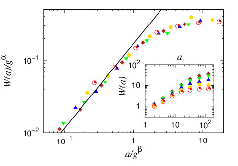
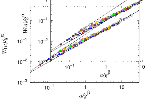
We now turn to large scaled Young modulus, i.e. stiff systems — or equivalently, softer systems on small length scales. Hence, fronts appear as in Fig. 1a. We set in the following $e=3.125$. The corresponding plot of averaged wavelet coefficient $W(a)$ vs. scale $a$ is shown in the insert in Fig. 3a. The different curves correspond to different gradients $g$ and $L$. Repeating the analysis of Sapoval et al. srg85 ; hbrs07 for gradient percolation, we assume that the front has an isotropic correlation length $\xi$ associated with it. In the case of gradient percolation, this correlation length is related to the gradient through the relation $\xi\sim g^{-\nu/(1+\nu)}=g^{-4/7}$, where $\nu=4/3$ is the percolation correlation length exponent. As was argued in Ref. shb03 , the same analysis may be repeated for correlated systems such as the present one, but with a possibly different $\nu$. We would then expect data collapse in Fig. 3a by rescaling $W(a)\to W(a)/\xi=W(a)/g^{-\alpha}$ and $a\to a/\xi=a/g^{-\beta}$, and where $\alpha=\beta=\nu/(1+\nu)$. We show in Fig. 3a, the data collapse that ensues when choosing $\alpha=\beta=4/7$, i.e., the ordinary uncorrelated percolation value $\nu/(1+\nu)$, where $\nu=4/3$. There are two distinct regions in the figure. For large values of $a/g^{-\beta}$, $W(a)/g^{-\alpha}$ is independent of $a/g^{-\beta}$. Hence, the front has the character of uncorrelated noise. We will discuss this further on. For small $a/g^{-\beta}$, the data follow a power law. We show in the figure (Fig. 3a) a straight line with slope $7/6=2/3+1/2$. Hence, the data are consistent with the fronts being self affine on these scales with roughness exponent

$$\zeta_{-}=2/3\;,$$ (6)

a value consistent with gradient percolation hbrs07 — and consistent with the experimental value reported by Santucci et al. sgtshm10 , $\zeta_{-}=0.60\pm 0.05$.

In order to further the analysis, we follow the procedure in hbrs07 by smoothening the fronts by removing the jumps due to the overhangs through the transformation

$$h_{i}(n)\to h_{i}^{k}(n)=$$

$$\sum^{i}_{m=0}\textrm{sgn}[h_{m+1}(n)-h_{m}(n)]\ |h_{m+1}(n)-h_{m}(n)|^{k}\;,$$

when $k\to 0$ bh07 . Hence, all steps are equal to one in $h_{i}^{0}(n)$, all overhangs have been removed. We ensure by this procedure that the scaling properties of the roughness are due to self affinity and not due to the overhangs which are prevalent in this regime.

We plot in Fig. 3b the rescaled $W(a)/g^{-\alpha}$ based on transforming $h^{0}_{i}$ vs. the rescaled $a/g^{-\beta}$. We have set $\alpha=\beta=4/7$, consistent with ordinary gradient percolation. The two straight lines that have been added to the figure have slopes $2/3+1/2=7/6$ and $1/2+1/2=1$ respectively. On small scales, the fronts are then self affine with a roughness exponent $\zeta_{-}=2/3$ — the gradient percolation value hbrs07 . On larger scales and with the overhangs removed, one would naively have expected to observe the fluctuating line regime characterized by a roughness exponent $\zeta_{+}=0.39$. However, by removing the overhangs, the effective roughness exponent one measures is $\max(1/2,\zeta_{+})$, which in this case is 1/2 bh07 . Fig. 3b, then, shows the crossover from a roughness exponent consistent with ordinary gradient percolation to a plain random walk exponent which is a result of the smoothening process.

Hence, we conclude that the scaling properties seen on small scales are consistent with uncorrelated gradient percolation. The analysis of Schmittbuhl et al. shb03 suggested a correlated gradient percolation process. This is one step further. We suggest that the process is an uncorrelated gradient percolation process on small scales where coalescence is the dominating process.

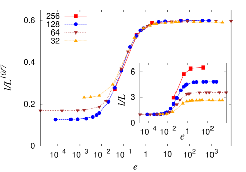
Roughness exponents are notoriously difficult to measure. The data presented in Fig. 3 are not of sufficient quality to warrant firm conclusions on the small-scale universality class by themselves. We therefore in the following measure the fractal dimension of the fronts. Leaving the SOS assumption, we now follow the front as shown in Fig. 1. The front has a length $l$. For small values of the scaled Young modulus $e$, there are no (or very few) overhangs and we expect $l$ to be proportional to $L$: it is not fractal. However, for large $e$ where overhangs are prevalent, we do expect it to be fractal. We assume that there is a correlation length $\xi$ and that the front is fractal up to this scale. Hence, the length of the front $l$ then scales as

$$l\sim\xi^{D_{f}}\ \left(\frac{L}{\xi}\right)\;.$$ (8)

From Sapoval et al. srg85 , we know that $\xi\sim g^{-\nu/(1+\nu)}$. We now set $g=c/L$, where $c$ is a constant. Hence, we find

$$l\sim L^{(\nu D_{f}+1)/(\nu+1)}\;.$$ (9)

If we are dealing with ordinary gradient percolation, $\nu=4/3$ and $D_{f}=7/4$ gr05 . Hence, we expect $(\nu D_{f}+1)/(\nu+1)=10/7\approx 1.43$. We show in Fig. 4, $l/L^{10/7}$ as a function of the scaled Young modulus, $e$. For large values of $e$, there is excellent data collapse. For small values of $e$, there is data collapse when $l/L$ is plotted against $e$, see the insert of Fig. 4, indicating that the front is not fractal in this regime. We are seeing the crossover from the coalescence-dominated regime to the fluctuating line regime as $e$ moves from large to smaller values. Since $e=E/L$, we may keep $E$ fixed and change $e$ by changing $L$. Hence, the coalescence regime is a small-scale regime whereas the fluctating line regime is a large-scale regime.

If we work backwards and search for the best scaling exponent to produce data collapse in Fig. 4, we find $l/L^{1.44}$. This gives $D_{f}=1.77\pm 0.02$, entirely consistent with the percolation value $7/4$.

Figure 4: Length of the fracture front $l$ scaled by system size plotted against effective Young modulus $e$. The main figure shows data collapse for $l/L^{10/7}$ for large $e$ values and the insert shows data collapse for small $e$ values for $l/L^{1}$. We set $g=1.6/L$. The data are based on 425000 fronts for $L=32$, 286482 fronts for $L=64$, 282022 fronts for $L=128$ and 32117 fronts for $L=256$.

Hence, we have through the use of a single model based on the fiber bundle model with a soft clamp and a gradient in the breaking threshold, been able to identify two mechanisms by which the fracture front propagates. On small scales, it is coalescence of damage the dominates, whereas on large scales the front advances as descibed by the fluctuating line model. The coalescence regime is in the universality class of ordinary percolation.

We are grateful for discussions and suggestions by D. Bonamy, K. J. Måløy and K. T. Tallakstad. We thank the Norwegian Research Council for financial support. Part of this work made use of the facilities of HECToR, the UK’s national high performance computing service, which is provided by UoE HPCx Ltd at the University of Edinburgh, Cray Inc and NAG Ltd, and funded by the Office of Science and Technology through EPSRC’s High End Computing Programme.

References

- (1) J. Schmittbuhl and K. J. Måløy, Phys. Rev. Lett. 78 3888 (1997).
- (2) J. Schmittbuhl, S. Roux, J.-P. Vilotte and K. J. Måløy, Phys. Rev. Lett. 74 1787 (1995).
- (3) J. P. Bouchaud, E. Bouchaud, G. Lapasset and J. Planès, Phys. Rev. Lett. 71 2240 (1993).
- (4) A. Rosso and W. Krauth, Phys. Rev. E. 65 R025101 (2002).
- (5) A. Delaplace, J. Schmittbuhl and K. J. Måløy, Phys. Rev. E. 60 1337 (1999).
- (6) D. Bonamy, J. Appl. Phys. D, 42, 214014 (2009).
- (7) D. Bonamy and E. Bouchaud, Phys. Rep. 498 1 (2011).
- (8) J. Schmittbuhl, A. Hansen and G. G. Batrouni, Phys. Rev. Lett. 90 045505 (2003).
- (9) E. Bouchaud, J. P. Bouchaud, D. S. Fisher, S. Ramanathan and J. R. Rice, J. Mech. Phys. Sol. 50, 1703 (2002).
- (10) S. Santucci, M. Grob, R. Toussaint, J. Schmittbuhl, A. Hansen and K. J. Måløy, Europhys. Lett. 92 44001 (2010).
- (11) A. Shekawat, S. Zapperi and J. P. Sethna, arXiv:1210.0989v1 (2012).
- (12) L. Laurson, S. Santucci and S. Zapperi, Phys. Rev. E, 81, 046116 (2010).
- (13) A. I. Larkin and Y. N. Ovchinnikov, J. Low Temp. Phys. 34, 409 (1979).
- (14) S. Pradhan, A. Hansen and B. K. Chakrabarti, Rev. Mod. Phys. 82, 499 (2010).
- (15) G. G. Batrouni, A. Hansen and J. Schmittbuhl, Phys. Rev. E. 65 036126 (2002).
- (16) K. L. Johnson, Contact Mechanics (Cambridge University Press, Cambridge, 1985).
- (17) G. G. Batrouni, A. Hansen and M. Nelkin, Phys. Rev. Lett. 57, 1336 (1986).
- (18) G. G. Batrouni and A. Hansen, J. Stat. Phys. 52, 747 (1988).
- (19) A. Stormo, K. S. Gjerden and A. Hansen, Phys. Rev. E, 86, R025101 (2012).
- (20) A. Hansen, Comp. Sci. Engn. 7, (5), 90 (2005).
- (21) B. Sapoval, M. Rosso and J. -F. Gouyet, J. Phys. Lett. 46, L149 (1985).
- (22) J.-F. Gouyet and M. Rosso, Physica A 357 86 (2005).
- (23) A. Delaplace, S. Roux and G. Pijaudier-Cabot, J. Engn. Mech. 127 646 (2001).
- (24) K. S. Gjerden, A. Stormo and A. Hansen, J. Phys: Conf. Series, 402, 012039 (2012).
- (25) A. R. Mehrabi, H. Rassamdana, and M. Sahimi, Phys. Rev. E 56 712 (1997).
- (26) I. Simonsen, A. Hansen and O. M. Nes, Phys. Rev. E 58 2779 (1998).
- (27) A. Hansen, G. G. Batrouni, T. Ramstad and J. Schmittbuhl, Phys. Rev. E. 75 030102 (2007).
- (28) J. Ø. H. Bakke and A. Hansen, Phys. Rev. E, 76, 031136 (2007).