Bound states of Dipolar Bosons in One-dimensional Systems

Abstract

We consider one-dimensional tubes containing bosonic polar molecules. The long-range dipole-dipole interactions act both within a single tube and between different tubes. We consider arbitrary values of the externally aligned dipole moments with respect to the symmetry axis of the tubes. The few-body structures in this geometry are determined as function of polarization angles and dipole strength by using both essentially exact stochastic variational methods and the harmonic approximation. The main focus is on the three-, four-, and five-body problems in two or more tubes. Our results indicate that in the weakly-coupled limit the inter-tube interaction is similar to a zero-range term with a suitable rescaled strength. This allows us to address the corresponding many-body physics of the system by constructing a model where bound chains with one molecule in each tube are the effective degrees of freedom. This model can be mapped onto one-dimensional Hamiltonians for which exact solutions are known.

1 Introduction

Heteronuclear molecules with strong electric dipole moments are a current pursuit of the cold atom community [1, 2, 3, 4, 5, 6]. The dipole-dipole forces in such systems can be externally controlled and give access to long-range and anisotropic interactions. Strong interactions can lead to rapid chemical reaction loss which can, however, be suppressed by considering low-dimensional trapping potentials [7, 8]. In the case of one or several one-dimensional tubes holding dipolar particles theoretical works indicate that a number of interesting physical states can be realized. Non-trivial Luttinger liquid states [9, 10, 11, 12, 13], superfluids, supersolids and stripes [14, 15, 16], liquids of trimers and crystals of different complexes [17, 18], Mott insulators [19, 20], exotic quantum criticality [21, 22], zig-zag transitions [23] and few-body states of several molecules [24, 25, 26] have been discussed in the literature.

In the current paper we will address the few-body structures that can be expected in an array of several tubes. A schematic setup for three tubes is shown in figure 1. The orientation of the dipolar molecules in the tubes can be controlled by an external electric or magnetic field depending on whether magnetic atoms or heteronuclear molecules are used. This opens up a host of interesting phenomena since the potentials of two dipoles in a single tube and the potential between two dipoles in different tubes change magnitude and sign as one changes the angles shown in figure 1.

Here we are concerned with the important question of existence of $N$-body bound states in multi-tube geometries. In order to address this we need to carefully consider the limits of small dipole moment and we consequently develop a perturbative approach to weakly bound states in one dimension that can handle the dipolar potential. At stronger coupling we consider a harmonic approximation. Both are compared to numerical results from the stochastic variational method that allow us to test the accuracy of the analytical formalism. A comparison is also made to exact results for $N$-body bosonic systems interacting through zero-range attractive forces, and we ask whether dipolar systems in one dimension approach the exact results in given limits and can in turn be effectively described by (properly renormalized) zero-range interactions. This is particularly important for many-body studies since zero-range interactions are not only convenient to work with but also often allow analytical results to be obtained. We also consider the two-body scattering dynamics of the dipoles and compare to zero-range results. Finally, we discuss the impact of our results for the many-body physics of dipolar bosons in one-dimensional geometries.

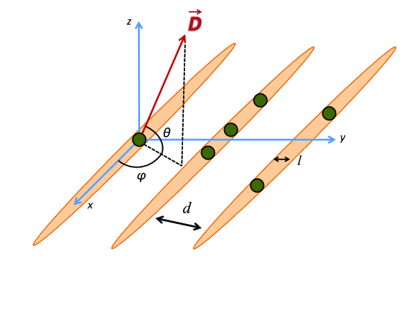
Figure 1: Schematic of the setup for the case of three equidistant one-dimensional tubes along the $x$-direction in the $xy$-plane with a distance between adjacent tubes of $d$. The dipolar moment, $\vec{\bm{D}}$, points along the direction specified by the two angles $\phi$ and $\theta$ as defined on the figure. Dark filled circles indicate the dipolar atoms in the tubes. The tubes have a thickness given by $l$. In typical experimental setups the tubes also have an in-tube confinement. This is indicated on the figure by the shrinking of the tubes at both ends. This in-tube confinement will, however, be neglected in this work.

2 Basic setup

We consider the setup depicted schematically in figure 1, i.e. an array of equidistant one-dimensional tubes containing dipolar particles with dipole moments aligned by an external field that does not interfere with the tubular geometry. The dipolar particles are identical bosons with mass $m$ and dipole moment $D$. The potential between two dipoles with coordinates $(0,0,0)$ and $(x,nd,0)$, $V(n,x)$, can be written in the form

$$\frac{md^{2}}{\hbar^{2}}V(n,x)=U\frac{\frac{x^{2}}{d^{2}}+n^{2}-3\cos(\theta)^{2}[\frac{x}{d}\cos(\phi)+n\sin(\phi)]^{2}}{(\frac{x^{2}}{d^{2}}+n^{2})^{5/2}},$$ (1)

where $d$ is the distance between two adjacent tubes and $n$ is an integer such that $nd$ is the intertube distance ($n=1$ for nearest neighbour (adjacent) tubes, $n=2$ for next-nearest neighbours and so on). Here we have defined the dimensionless dipole coupling strength, $U=\frac{mD^{2}}{\hbar^{2}d}$, where $D$ is the dipole moment (absolute value of the vector $\vec{\bm{D}}$ in figure 1). For $n=0$ we get the intratube interaction in the limit where the tubes are strictly one-dimensional. In experimental setups, arrays of one-dimensional tubes are constructed by applying optical lattices to the dipolar gas [7, 8]. In this case the tubes are not strictly one-dimensional but will have some width along the transverse direction that is determined by the laser intensity. This can be translated into a gaussian wave packet in the transverse direction that will be increasingly localized in space as the laser intensity increases. An effective interaction that takes this into account by integrating out a gaussian wave packet can then be obtained [25], which will in the limit of zero gaussian width reduce to the expression in (1). We will assume that the lattice is very strong so that the strict one-dimensional expression above is valid for the interaction of particles in different tubes which is accurate when the transverse width, $l$, is much smaller than the intertube distance, $d$. Corrections to this picture have been discussed in references [24] and [25]. Below we will return to the question of finite transverse width when we treat bound states with more than one particle per tube. From here on we will adopt units $\frac{\hbar^{2}}{md^{2}}$ and $d$ for all energies and lengths.

The potential above has the interesting property that for the case of $n\geq 1$

$$\frac{md^{2}}{\hbar^{2}}\int_{-\infty}^{\infty}V(x,n)dx=\frac{2U}{n^{2}}\left[\cos^{2}(\theta)\cos^{2}(\phi)-\cos(2\theta)\right],$$ (2)

and as a function of the angles we thus see that we can obtain both positive and negative values of the integrated interaction. The criterion for the existence of a two-body bound dimer in the limit of small $U$ is a negative integral [27, 28]. We thus see that one can control the presence of a weakly-bound dimer by changing $\phi$ and $\theta$. Below we will mostly address the situation where $\phi=\pi/2$ and $\theta=0$, i.e. dipoles that are oriented perpendicular to the tubes. In this case, the integral in (2) is $-\frac{2U}{n^{2}}$ and this means that the system can produce bound dimers between any two particles that are located in different tubes for any $n>0$.

However, if a given few-body state has more than one particle in a single tube, then the interlayer interaction will be either attractive or repulsive depending on the sign of $1-3\cos^{2}(\theta)\cos^{2}(\phi)$ (see (1) with $n=0$). Here we will only consider the regime where this quantity is positive, i.e. the case for which two dipoles in a single tube repel each other in order to avoid any collapsing states within the tubes.

3 Few-body bound states

We now present our results for up to five dipolar bosonic particles in multi-tube geometries. The discussion will involve analytical tools for addressing the limits of weak and strong dipolar interactions which will be compared to numerics using the exact stochastic variational approach [29, 30]. This allows us to determine the range of validity of the analytical methods that we employ. Along the way we will make a detailed comparison between the one-dimensional case with tubes and the two-dimensional case of multiple layers [7, 31, 32, 33, 34, 35, 36, 37]. We will also compare to the results of McGuire [38] for the exact ground state energy of an $N$-boson system with pairwise zero-range interactions in one dimension. Finally, we will investigate few-body states with more than one particle in a single tube for both the case of perpendicular dipoles ($\theta=0$ and $\phi=\pi/2$) and with tilted angles ($\theta=0$ and $\phi<\pi/2$).

3.1 Two-body states of two dipoles in two tubes

The first case is one dipolar particle in each of two adjacent tubes with dipole moments oriented perpendicular to the tubes ($\phi=\pi/2$ and $\theta=0$). This configuration has the Schrödinger equation

$$\left(-\frac{\partial^{2}}{\partial x^{2}}+U\frac{x^{2}-2}{(x^{2}+1)^{5/2}}\right)\Phi=\epsilon\Phi,$$ (3)

where $x$ is the relative distance of the two dipoles along the tube axis, $\epsilon$ is the eigenenergy in units of $\frac{\hbar^{2}}{md^{2}}$ and $\Phi$ is the wave function. We start with the analytically accesible limits of strong $\epsilon/U\sim 1$ and weak $\epsilon/U\ll 1$ binding.

Weak binding. From reference [28] we know that a bound state exists for potentials that fulfil $\int(1+|x|)V(x)dx<\infty$. For this bound state we write the solution of (3) in the form

$$\Phi(\kappa,x)=e^{-\kappa x}-\int_{x}^{\infty}\mathrm{d}y\frac{\sinh(\kappa[x-y])}{\kappa}V(y)\Phi(\kappa,y),$$ (4)

where $\epsilon=-\kappa^{2},\kappa>0$ [39]. Notice that we are ’normalizing’ the wave function at $x=\infty$ and the integrating our way to any other value of $x$. For $x<0$ the term $e^{-\kappa x}$ appears to diverge, but the second term will also contribute and the combination yields the correct answer. We now obtain the equation for the binding energy

$$\kappa=-\frac{1}{2}\int_{-\infty}^{\infty}\mathrm{d}ye^{\kappa y}V(y)\Phi(\kappa,y).$$ (5)

For weak binding this can be solved iteratively for small $\kappa$, i.e.

$$\kappa=-\frac{1}{2}\int_{-\infty}^{\infty}V(y)\mathrm{d}y+\frac{1}{2}\int_{-\infty}^{\infty}\mathrm{d}yV(y)\int_{y}^{\infty}\mathrm{d}y^{\prime}(y-y^{\prime})V(y^{\prime})+\ldots$$ (6)

Here we have used that $\Phi(\kappa,y)\approx 1+O(\kappa)$. Upon inserting the potential in (1) with $n=1$ and carrying out the integrals we find

$$\kappa=U+U^{2}\frac{\pi}{16}+o(U^{2}),$$ (7)

which implies that to leading order in $U$, $\epsilon=-\kappa^{2}\propto-U^{2}$. These results were initially discussed by Landau [27] and Simon [28] but the procedure we present here allows simpler access to the higher-order terms. We note that the first term in (6) corresponds to a delta-function potential $-g\frac{\hbar^{2}}{md^{2}}\delta(\frac{y}{d})$ with $g=2U$ (where we have reintroduced explicit units for clarity). Numerically we find that this potential gives good approximation for the real potential with $U<0.2$. This is a valuable conclusion for studies that depend on a delta-function representation of the dipolar interaction in one dimension in order to describe many-body physics [21].

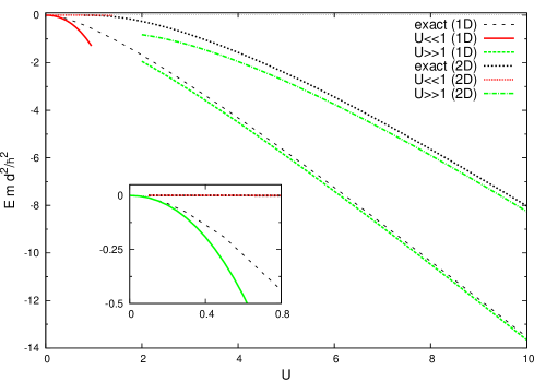
Figure 2: Energy, E, in units of $\frac{md^{2}}{\hbar^{2}}$ as a function of dimensionless dipolar strength, $U$. Comparison between exact numerical solution of the Schrödinger equation (3) and analytical predictions from table 1 for 1D and 2D. The inset is a magnification of the small $U$ regime. Note that the huge difference at small $U$ between 1D and 2D due to the exponential decrease of the binding energy at small coupling strength in 2D.

A clear difference to the 2D case is seen at this point. The weak-binding result in 1D is $\epsilon\propto-U^{2}$, whereas in 2D it is $\epsilon\propto-\exp(-8/U^{2})$ [29, 33, 34, 35]. This is consistent with our expectation that weakly-bound 1D dipolar few-body bound states are generally more stable than similar systems in 2D, and any sort of external perturbations would have a less severe effect in the 1D setup.

We can also consider the case where $U<0$ corresponding to one of the dipoles in the two tubes pointing in opposite directions which should be possible to achieve using AC fields [40]. In this case the 2D setup with two adjacent planes will always have a bound dimer [30], whereas in 1D we find numerically that it takes a finite strength $U<-4.98$ to bind the two-body system. We can understand the latter if we consider $\kappa=0$ in (5). This transforms the condition for the appearance of the bound state. For small $U$ we have $U+U^{2}\frac{\pi}{16}=0$, which has two solutions; one corresponds to bound states with $U>0$ and another for bound states with $U<-\frac{16}{\pi}\sim-5.09$. The latter is within 2 percent of the numerical value. However, notice that the $U<0$ case opens up the possibility of binding and unbinding the dimer by tuning $U$ as originally envisioned in reference [31].

Strong binding 1D For this case we may assume that our wave function is strongly localised near the origin, i.e. $\langle x^{2}\rangle/\epsilon\rightarrow 0$, such that the probability to be in the classically forbidden region is small. Under these conditions we can use standard techniques to obtain the binding energy and the wave function. First we decompose the potential near the origin

$$U\frac{x^{2}-2}{(x^{2}+1)^{5/2}}=-2U+6Ux^{2}-45Ux^{4}/4+U\sum_{n=3}^{\infty}\alpha_{n}x^{2n}.$$ (8)

Using the assumption of strong localization we see that up to terms $O(\frac{1}{\sqrt{U}})$ we can solve the harmonic oscillator problem for the first two terms and include the third term via perturbation theory. This yields

$$\epsilon=-2U+\sqrt{6U}-45/32+O(\frac{1}{\sqrt{U}}).$$ (9)

A comparison of the numerical results for all values of $U$ to the weak and strong binding expansions is shown in figure 2. Both the limit of weak and strong binding are well reproduced by the different approximation schemes. We see differences between numerical and analytical results only around $U=1$. For completeness we also summarize all the analytical results and their regimes of validity in table 1

	1D
$\frac{md^{2}}{\hbar^{2}}\int V\mathrm{d}\mathbf{r}$	-2U
small $U>0$	$\epsilon=-U^{2}-\frac{\pi}{8}U^{3}+o(U^{3}),(U<0.2)$
large $U>0$	$\epsilon=-2U+\sqrt{6U}-45/32+O(\frac{1}{\sqrt{U}}),(U>4)$
	2D
$\frac{md^{2}}{\hbar^{2}}\int V\mathrm{d}\mathbf{r}$	0
small $|U|>0$	$\epsilon=-4\exp({-2\gamma-\frac{8}{U^{2}}+\frac{128}{15U}-\frac{2521}{450}+o(U)}),(U<0.8)$
large $U>0$	$\epsilon=-2U+\sqrt{24U}-15/4+O(\frac{1}{\sqrt{U}}),(U>7)$

Table 1: Comparison between 1D and 2D binding energies of two dipoles in two different layers or tubes with perpendicularly oriented dipole moments. The regimes of validity of the different analytical formulae are indicated in the parenthesis.

3.2 $N$-body Chains

We now proceed to discuss the case where we have $N$-body chains that consist of one dipolar particle in each of $N$ adjacent layers or tubes. In the 2D case, these sorts of structures have generated a lot of recent interest since one expects highly non-trivial few- and many-body dynamics [31, 33, 41, 42, 43, 44, 45, 46]. There is a similar interest in the one-dimensional multi-tube configurations [15, 19, 21, 22]. The Hamiltonian for the $N$-body 1D system is

$$H=\sum_{i=1}^{N}\frac{p_{i}^{2}}{2m}+\sum_{i>j}V(x_{ij},n_{ij}),$$ (10)

where $x_{ij}$ is the relative distance of the $i$th and $j$th particles along the tube direction and $n_{ij}$ is the integer that signifies how far apart the tubes are that hold the $i$th and $j$th particles ($n=1$ for adjacent tubes and so on). For the case where the pair-wise potentials of equal strength and zero-range, this Hamiltonian was studied in the classical papers of Lieb and Liniger [47, 48]. McGuire has shown that for this delta-function case, the bound state energy, $E_{N}$, of the $N$-body problem can be written very elegantly as $E_{N}/E_{2}=N(N^{2}-1)/6$, where $E_{2}$ is the two-body bound state energy of the same delta-function potential [38].

Here we consider a system of $N$ dipoles placed in $N$ different tubes with the potential in (10) given by (1). This is intrinsically a case with long-range interactions which has also generated some classical studies. In the particular case where the interaction behaves as $r^{-2}$ this is the Sutherland-Calogero model [49, 50]. In the present case with dipoles we have a long-range tail that behaves as $r^{-3}$. We would like to build a connection to the zero-range studies for the dipolar systems in 1D. For general polarization angles, however, the interactions are anisotropic and more difficult to compare to the isotropic zero-range models. In this section we therefore study the case of perpendicular polarization ($\phi=\pi/2$ and $\theta=0$) where the anisotropy is absent.

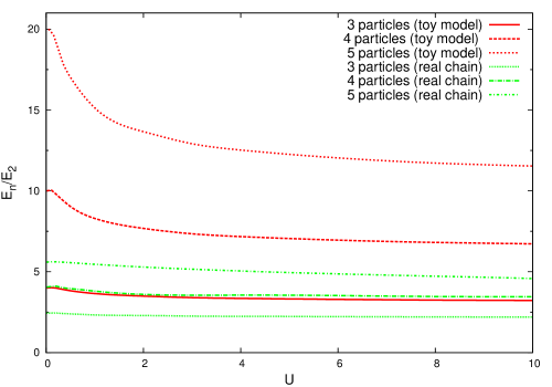
Figure 3: Numerically determined $N$-body binding energies relative to the two-body energy, $E_{2}$, as function of coupling strength, $U$, for $N$-body chains using both a toy model where all interactions have $n=1$ in (1) and the realistic case where $n$ is different for different pairs of particles in the chain.

As we have demonstrated above, for $U<0.2$ we get universal behaviour in a sense that the potential $\frac{md^{2}}{\hbar^{2}}V=-2U\delta(\frac{x}{d})$ accurately describes our system. Now we want to establish how well this zero-range approximation works on the few-body level with $N>2$. To do so we first consider a toy model where all $N$ particles interact with the same interaction corresponding to $n=1$ in (1). This is precisely the case where it makes sense to compare to the analytical result $E_{N}/E_{2}=N(N^{2}-1)/6$. In this way we can get a feeling for when the zero-range approximation works. For realistic chains $n$ is not always equal to one. This means that these are easier to describe using a zero-range approximation since particle pairs that are located several tubes apart in a chain have a potential that effectively correspond to a smaller value of $U$ (as compared to the $n=1$ case).

The numerically calculated chain binding energies relative to the two-body energy, $E_{N}/E_{2}$, for both the toy model and the real dipolar chains in 1D are presented in figure 3. We observe the delta-function behaviour in all cases for $U<0.15$, and the strong coupling behavior is slowly approached with increasing interaction strength. In current experiments with ⁴⁰K-⁸⁷Rb molecules [7, 8], we have $U\lesssim 0.1$ so this is weak-coupling in the current context. In the strong coupling limit, the leading term for the toy model is $E_{N}/E_{2}=\frac{N(N-1)}{2}$ which is simply the number of pairs that all contribute an energy $E_{2}$. For the realistic chain, the expression is instead

$$E_{N}/E_{2}=\sum_{k=1}^{N}\sum_{i=1}^{N-k}\frac{1}{i^{3}}=NH_{N-1}^{(3)}-H_{N-1}^{(2)},$$ (11)

where $H_{m}^{(k)}=\sum_{i=1}^{m}i^{-k}$ is the harmonic number of order $k$. We will elaborate more on the strong-coupling limit below.

We see a large difference between the toy model and the real chain in figure 3 in the weak-coupling limit $U\ll 1$. This is an important conclusion of our work that has implications for many-body studies on dipolar systems that work with delta-function approximations for the dipolar interactions. The toy model is relevant for an equidistant triangular tube configuration as studied in reference [21]. Our results for this $N=3$ case show a very flat profile for all values of $U$ and from the point of view of energetics it is thus a reasonable approximation to use the delta-function $\frac{md^{2}}{\hbar^{2}}V(x)=-2U\delta(\frac{x}{d})$. The $N=4$ and $5$ would be applicable to a tube configuration with four and five nearest-neighbours respectively (the latter would of course not be possible with standard crystal lattices). However, in these cases the variation of the energies with $U$ is much more drastic, indicating that a zero-range description is only good for very small $U$.

For the real chain systems, the curves are rather flat for all $N$. This is connected to the fact that the terms with $n>1$ in (10) will give a contribution that is suppressed. Due to the flatness of the curves in figure 3, we can get a good approximation for the $N$-body binding energy of the realistic chains by using an effective model for $N$-body systems with $\frac{md^{2}}{\hbar^{2}}V(x)=-2U_{eff}(N)\delta(\frac{x}{d})$ where

$$U_{eff}(N)=\frac{6}{N(N^{2}-1)}\left[NH_{N-1}^{(3)}-H_{N-1}^{(2)}\right]U.$$ (12)

The blessing of working with a zero-range interaction comes at the price of having an $N$-dependent coupling. This ensures that the $N$-body bound states present in this geometry are properly described. We will use this effective dipolar strength to study the corresponding many-body system below. We stress that the delta-function approximation with $U_{eff}(N)$ coupling is only accurate for weak interaction, i.e. small $U$. In the case of $N=5$ from $U\to 0$ and up to $U=10$ we find a difference of about $20\%$ on the value while for $N=3$ and $N=4$ the difference is slightly less. So the flatness and thus the reliability of the delta-function approach is on the level of $20\%$ for $U\leq 10$ and $N\leq 5$. It is very important to notice that we reproduce the strong-coupling limit, i.e. large $U$, with this choice of $U_{eff}$. This means that if we use the potential in (12) as an effective potential between $N$ bosonic particles in one dimension, we obtain the correct strong-coupling binding energy (11). This all builds on the flatness of the energy in figure 3 and is only as good as the uncertainty quoted above. This is important to notice as below we will look at low-energy many-body physics using this effective interaction.

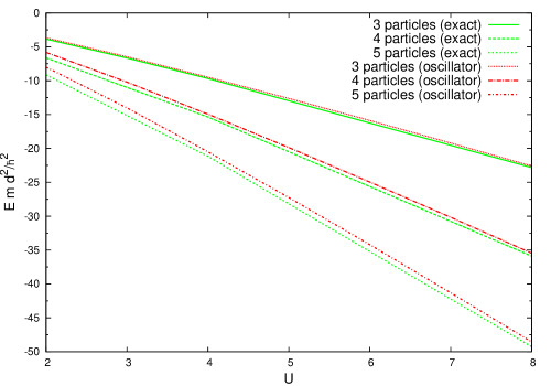
Figure 4: Energy, E, in units of $\frac{md^{2}}{\hbar^{2}}$ as a function of dimensionless dipolar strength, $U$. Comparison between exact numerical calculations obtained from the stochastic variational approach and the oscillator approximation described in the text for the case of perpendicular dipoles, i.e. $\phi=\pi/2$ and $\theta=0$ for the case of $N=3$, $4$ and $5$.

Chains in the oscillator approximation As we have seen for small $U$, the zero-range approximation gives reliable results. However, we would also like to discuss the strong binding limit where $U\gg 1$ and provide a simple analytical procedure for obtaining the energies and wave functions. This can be done using exact harmonic models [51, 52] where the full two-body interaction (the dipolar interaction in this case) is represented by a harmonic oscillator with parameters that are carefully chosen to reproduce energetics and structure at the two-body level [45]. We expect this to be a good approximation for $U\gg 1$ since the potential in (1) has a deep pocket in this case. However, it turns out that this approximation can be very accurate even for moderate $U$ in the case of 2D multi-layered systems with chains [53].

In figure 4 we show a comparison of the oscillator approximation to exact numerical calculations for the case of perpendicularly oriented dipoles ($\phi=\pi/2$ and $\theta=0$). Note that the horizontal axis begins at $U=2$ (for $U<2$ the oscillator does not reproduce the exact results well). We get a very good agreement for $N=3$, while for higher particle numbers there is a clearly visible deviation. This stems from issues with the two-body interactions coming from the outermost tubes where the oscillator approximation starts to fail since the contributions are not well-described by an oscillator (the effective $U$ for these terms is small for any $U$ value considered here). However, the overall agreement is still within a few percent for $U>5$. One way to improve the agreement for higher particle numbers could be to introduce an effective three-body force (more generally an $N$-body force) in addition to the two-body potential terms. Such an approach is very common in nuclear physics and in effective field theory studies of universal three-body physics [54, 55].

We now change the angle $\phi$ to investigate the effects of anisotropy. Figure 5 shows the case with $\phi=\phi_{m}$ and $\theta=0$, where $\phi_{m}$ satisfies $\cos^{2}\phi_{m}=\frac{1}{3}$. Recalling the discussion after (1) this implies that the potential between two dipoles in the same tube vanishes. First we observe that the overall energy scale becomes smaller, because the depth of the potential and net volume of the potential is smaller than for the perpendicular polarization case in figure 4. For $N=3$ and $N=4$ we again see very good agreement between the oscillator approximation and the numerics. The largest chain with $N=5$ shows what appears to be an even better agreement than for the $\phi=\pi/2$ and $\theta=0$ case. What is also striking is that the oscillator results and the numerics cross around $U\sim 5$. This happens since our method ensures that the oscillator reproduces the slope of the numerical results in the limit $U\gg 1$ (as discussed for the 2D case in reference [53]). The optimization of the parameters for the two-body oscillator potential for $2\leq U\lesssim 5$, however, produces a slightly different slope and a crossing thus takes place.

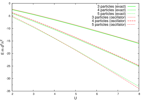
Figure 5: Energy, E, in units of $\frac{md^{2}}{\hbar^{2}}$ as a function of dimensionless dipolar strength, $U$. Same as in figure 4 but for the case where $\phi=\phi_{m}$ and $\theta=0$. This corresponds to vanishing intratube interaction, i.e. two dipolar particles in the same tube do not interact.

3.3 Non-chain bound complexes

We now consider the case where there are two particles in one tube. The simplest configuration of this sort is two tubes with three particles in total, i.e. one particle in one tube and two particles in the adjacent tube. At this point we need to take the width of the tube that we discussed in section 2 explicitly into account in order to work with an intratube interaction that best describes the experimental situation. This can be done by folding the potential with a gaussian wave packet of width $l$ that represents the wave function of the system in the transverse direction (along the $y$-axis in figure 1) This yields the intratube interaction [25]

$$V_{rep}(x)=U_{rep}\lambda^{3}(1-3\cos^{2}\phi\cos^{2}\theta)f(\lambda x),$$ (13)

where

$$f(z)=\frac{-2|z|+\sqrt{2\pi}(1+z^{2})\exp(z^{2}/2)\mathrm{erfc}(|z|/\sqrt{2})}{4},$$ (14)

and $\lambda=d/l$ and $U_{rep}$ is the strength of the intratube interaction. This means that the intratube potential has been regularized by the finite width of the transverse confinement and does not have the strict 1D form $x^{-3}$ expect in the limit of $\lambda\to\infty$. In a system where the dipole moment is the same for all particles in all tubes we have $U_{rep}=U$, where $U$ is the strength of the intertube interaction. The dipole orientation and the induced dipole moment is typically controlled by applying an external electric or magnetic field that is constant across the whole system. However, if one applies also a field gradient then it should be possible to obtain a system where the induced dipoles moment varies from tube to tube (or layer to layer in the 2D multilayer case). In this case we can have a situation where $U_{rep}\neq U$ and we thus vary both quantities independently in the current study. As discussed previously, we will consider only the repulsive case where $1-3\cos^{2}\phi\cos^{2}\theta>0$ in order to avoid possible intratube collapse of the system. Unless explicitly states, we use $\lambda=5$ everywhere (see reference [25] for a discussion of the effects of changing $\lambda$).

We start by considering the case where all particles are perpendicularly polarized, i.e. $\phi=\pi/2$ and $\theta=0$. Observe that if $U_{rep}=0$ we have a trimer energy that is below the dimer energy, and if $U_{rep}\to\infty$ we can not bind three particles. We now want to find the value $U_{rep}^{cr}$ at which the three-body system is bound for a given value of $U$, so we keep $U$ fixed and vary $U_{rep}$. In reference [36] it has been shown that $U_{rep}^{cr}/U$ is an increasing function of $U$ by an argument that does not depend on the dimensionality and thus applies equally well to layers in 2D and tubes in 1D. In turn we only need to consider $U\rightarrow\infty$ to obtain an upper bound for $U_{rep}^{cr}/U$. This upper bound is a decreasing function of $\lambda$ and for $\lambda=5$ we get $U_{rep}^{cr}/U<0.41$. In order to find the lower bound for $U_{rep}^{cr}/U$ we will use the variational principle with a normalised three-body wave function of the form $\Psi(x,y)=\Phi(x)\varphi(y)$, where $\Phi(x)$ is the normalised dimer wave function and we have used Jacobi coordinates $\sqrt{2}x=x_{1}-x_{2}$ and $\sqrt{3/2}y=x_{3}-(x_{1}+x_{2})/2$. From this we obtain the upper bound for the three-body energy

$$E_{3}^{var}=\langle\Psi|H_{3}|\Psi\rangle=E_{2}+$$

$$\langle\varphi|\bigg{(}T_{y}+\int\Phi^{2}(x)\bigg{[}V_{rep}(|\sqrt{\frac{1}{2}}x+\sqrt{\frac{3}{2}}y|)+V(|\sqrt{\frac{1}{2}}x-\sqrt{\frac{3}{2}}y|)\bigg{]}\mathrm{d}x\bigg{)}|\varphi\rangle,$$ (15)

where the kinetic term for the $y$ coordinate is $T_{y}=-\frac{\hbar^{2}}{2m}\frac{\partial^{2}}{\partial y^{2}}$. Here $V_{rep}$ is given in (13) and $V$ is given by (1) with $n=1$. Equation (5) in principle allows us to estimate where $E_{3}^{var}<E_{2}$ holds, which gives us the lower bound for $U_{rep}^{cr}$. However, in general this equation is not easy to analyse so we obtain the lower bound using the simpler condition for the effective potential acting on $\varphi$ in (15) which is that it must have negative net volume. The limit of zero net volume requires

$$\int\int\Phi^{2}(x)\bigg{[}V_{rep}(|\sqrt{\frac{1}{2}}x+\sqrt{\frac{3}{2}}y|)+V(|\sqrt{\frac{1}{2}}x-\sqrt{\frac{3}{2}}y|)\bigg{]}\mathrm{d}x\mathrm{d}y=0,$$ (16)

which can be simplified to

$$\int\bigg{[}V_{rep}(y)+V(y)\bigg{]}\mathrm{d}y=-2U+U_{rep}\lambda^{2}\int_{-\infty}^{\infty}f(y)\mathrm{d}y=-2U+\lambda^{2}U_{rep}=0.$$ (17)

This lower bound is a decreasing function of $\lambda$, and for $\lambda=5$ we get $U_{rep}^{cr}/U>2/25$. Collecting our results, we have for $\lambda=5$ that $0.41>U_{rep}^{cr}/U>2/25$. This means that if we could manipulate the values of the intratube and intertube interactions independently, we could create or destroy the three-body bound state in two tubes with perpendicular polarization. This effect is completely due to the finite range of the potential, because for zero-range potentials any value $U_{rep}/U$ will produce a bound state (the system becomes equivalent to the fermionic states studied by McQuire in reference [56] for which a bound state always exists).

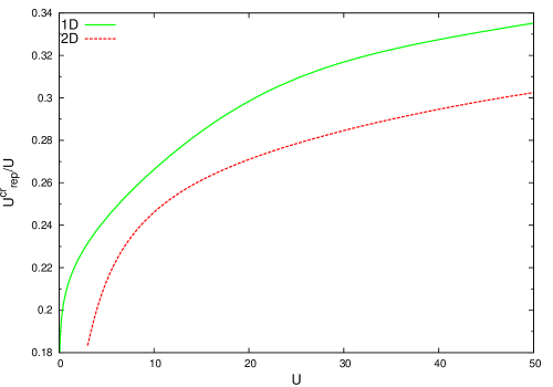
Figure 6: Ratio $U^{cr}_{rep}/U$ as a function of U at which a three-body state with two dipoles in one tube (plane) and one in the adjacent tube (plane) becomes possible in 1D (2D). The three-body state exists below the lines in the plot. The lines drops sharply to zero for small $U$. Here we use $\lambda=5$.

In figure 6 we show the critical value, $U_{rep}^{cr}/U$, as a function of $U$ for both the case of 1D tubes and for comparison we also plot the results of the same study for a bilayer in 2D [36]. Both of these calculations have been done with $\lambda=5$. We see a clear difference between the critical values for three-body bound state formation in the two cases with the 1D situation allowing for larger repulsive interactions. This is connected to the price one pays for localizing particles in a bound states complex. In 2D we need to localize in two independent directions which is more expensive than 1D. As expected, 1D tubes are more favourable for formation of these larger complexes.

Having discussed how a tuning of the intratube repulsion can bind a three-body state, we now consider an alternative route to bind this state which is by tilting the angle, $\phi$. We assume that $U_{rep}=U$, and are looking for values of $\phi$ and $U$ for which a bound state exists. For a given angle $\phi$ we introduce the notation $U^{cr}(\phi)$ which is the value at which the two-body dimer (one particle in each of two adjacent tubes) energy is equal to the three-body energy which defines the threshold. We start with three particles as before but tilted by angles $\theta=0,\phi\in[\phi_{m},\pi/2]$. We already proved that for $\phi=\pi/2$ we do not have a bound state if $U_{rep}=U$. However, we know that for $\phi=\phi_{m}$ we always have a three-body bound state, because the intralayer interaction vanishes. This implies that there is a range of angles where the three-body state exists.

To approach this problem analytically, we can calculate the net volume as above. This yields

$$\int\bigg{[}V_{rep}(y)+V(y)\bigg{]}\mathrm{d}y=2U(\cos^{2}\phi-1)+U(1-3\cos^{2}\phi)\lambda^{2}.$$ (18)

Putting it to zero we obtain the smallest angle below which the three-body bound state exist for any value of $U$. The condition for a three-body bound state is $\phi\leq\cos^{-1}(\sqrt{\frac{\lambda^{2}-2}{3\lambda^{2}-2}})$ which in the case of $\lambda=5$ yields $\phi\lesssim 0.975$ or $55.9^{o}$. In the strict 1D limit where $\lambda\to\infty$, we find the result $\phi\leq\phi_{m}$. The function $\frac{\lambda^{2}-2}{3\lambda^{2}-2}$ is decreasing with $\lambda$ which is a result of the behaviour of the function in (14) which has a finite value for zero argument for any finite $\lambda$. In strict 1D we expect that the repulsion will not allow this three-body bound state due to the cubic singularity $x^{-3}$ of the repulsive potential. For the more realistic case with a finite $\lambda$ we can have bound states for angle in the regime $\phi>\phi_{m}$ as well. An additional bound can be found by using classical arguments, i.e. neglecting kinetic energy in the Schrödinger equation and studying just the potential landscape [36]. This yields a bound of $\phi\gtrsim 1.15$ or $66^{o}$ so that for any $U$ we do not have three-body bound states in the case where $U_{rep}=U$. In summary, we have found that for $\phi_{m}<\phi\lesssim 1.15$ there exist a value of $U^{cr}(\phi)\in[0,\infty)$, such that for $U>U^{cr}(\phi)$ the bi-tube trimer is bound.

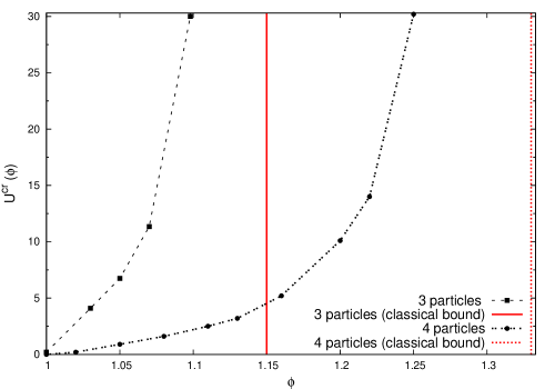
Figure 7: Critical value, $U^{cr}(\phi)$, where the trimer in two tubes (one and two particles) and tetramer in three tubes (one, two and one particles) dissociates as function of the tilting angle $\phi$ for $\theta=0$. The dissociation thresholds where calculate at the dots and squares with connecting lines to guide the eye. The vertical lines mark the angles beyond which a classical calculation (neglecting kinetic energy for all particles) predicts no bound states can occur because the system is overall repulsive.

In figure 7 we plot $U^{cr}$ as a function of $\phi$ for three particles in two tubes in the case where $U_{rep}=U$, i.e. the case of current experimental interest where the dipole strength is controlled by one external field that is constant over the entire samples. The points indicate the values at which the dissociation points have been obtained numerically (connecting lines are a guide to the eye). The three-body bound states are present on the left-hand side in the diagram since here the intratube repulsion is not strong enough to break the bound state apart. The results obtained here are consistent with results reference [25] for $U<15$ where a comparison can be made. For $U>15$ we find a very sharp increase in $U^{cr}(\phi)$ that takes place at $\phi\sim 1.1$, a few degrees before a classical calculation renders the system unbound at $\phi=1.15$.

In order to address the question of additional tubes and their effect on bound states with more than one particle per tube, we have also consider a four-body state in three tubes (as in figure 1) with two dipoles in the middle tube and one in each of the two outer tubes. The results are also presented in figure 7. We again see a sharp increase for large $\phi$ before we get to the classically unbound value of $\phi=1.34$ or $76.5^{o}$. However, there is a significant increase of region in which bound state with two particles in a single tube are present due to the extra attraction from adding a particle in an adjacent tube on the other side of the complex as compared to the three-body system with two and one in two tubes. Other four-body states can occur in two tubes as discussed in reference [25], but the parameter regime is severely suppressed due to the extra repulsion in the three-plus-one and two-plus-two four-body states in two tubes. We therefore expect that the case of three tubes could have interesting ’quasi’-Wigner crystal states for large $U$ beyond the clustered states studied in reference [18] where the clusters are not of the same size in each tube (here with cluster size one in the outer tubes and two in the inner tube). We can continue this kind of game for five tubes in a one-two-one-two-one configuration and so on.

4 Scattering

While we are mainly concerned with negative energy bound state structures in this paper, we now present a short overview of some scattering results that can be deduced directly based on the formalism we introduced above. One basically only needs to make an analytical continuation of the bound state discussions above in order to arrive at results for scattering of dipolar bosons in 1D tubes. Since current experiments with cold molecules aim for the low temperature regime where quantum degeneracy can be reached, we will focus exclusively on the low-energy scattering regime here.

The formal solution of the scattering problem, $\Psi$, satisfies the equation

$$\Psi(k,x)=e^{ikx}-\int_{x}^{\infty}\mathrm{d}y\frac{\sin(k[x-y])}{k}V(y)\Psi(k,y),$$ (19)

where the boundary condition is an out-going flux to the right with coefficient one of the form $e^{ikx}$ [39]. Here we define the reflection, $R(k)$, and transmission, $T(k)$, coefficients through $\Psi(k,x\rightarrow-\infty)=T(k)^{-1}e^{ikx}+\frac{R(k)}{T(k)}e^{-ikx}$ to be consistent with standard 1D potential scattering. By taking the limit $x\to-\infty$ we obtain

$$T(k)=\frac{2ik}{2ik-\int_{-\infty}^{\infty}\mathrm{d}xV(x)e^{-ikx}\Psi(k,x)}.$$ (20)

For $k=i\kappa,\kappa>0$, poles of $T(k)$ define bound states with the binding energy defined through the equation

$$\sqrt{(-\epsilon)}=\kappa=-\frac{1}{2}\int_{-\infty}^{\infty}\mathrm{d}ye^{\kappa y}V(y)\Psi(\kappa,y),$$ (21)

which is consistent with (5) and allows us to use the same techniques as before to obtain iterative improvements of the solution.

Consider now the case of dipoles oriented perpendicular to the layers, i.e. $\phi=\pi/2$ and $\theta=0$. In the limit of weak binding and low-energy scattering, $U\ll 1$ and $kd\ll U$, we find for the transmission coefficient of two particles in the two different tubes

$$T=i\frac{k}{\kappa_{b}},$$ (22)

and for the case of two particles in the same tube we find

$$T=-i\frac{kd}{U\lambda^{2}}.$$ (23)

These results are deceptively simple, yet they contain all the information about the dipolar physics in one-dimensional tubes at low energy in the small $U$ limit. As expected they vanish with $k$ as $k\to 0$ which is a manifestation of the Wigner threshold law. Also, as $\kappa_{b}\propto U$ in the weak-coupling limit (see table 1), we see that both expressions become large at very small $U$. This makes sense since the potential becomes very weak (and likewise the derivative of the potential). We also see that in the strict 1D limit, $\lambda\to\infty$, the transmission is completely suppressed and total reflect is expected. This is the emergence of the impenetrable boson regime called the Tonks-Girardeau limit [57, 58]. This limit can be studied with dipolar bosons in a 1D setup with an (in-tube) harmonic trap as discussed in reference [59].

Since we would like to obtain an effective model for dipolar systems of $N$-chains using zero-range interactions, we need to relate the transmissison coeffecients above to its zero-range equivalent. If we write the potential as $V(x)=g\delta(x)$, we find

$$T(k)=\frac{2ik}{2ik-\frac{mg}{\hbar^{2}}}\to-\frac{2ik\hbar^{2}}{mg},$$ (24)

for low-energy scattering. We see that we recover the $g=-2U$ result for the case of two dipoles in different tubes (using our units of energy and length given in section 2) and we find $g=U\lambda^{2}$ for dipoles in the same tube.

5 Many-Body Physics

We now want to address the case of a many-body system of $N$ adjacent tubes with $M$ particles in each tube. We will focus on the case of perpendicular orientation of the dipoles with respect to the tubes ($\theta=0$ and $\phi=\pi/2$) and comment on the case of general angles in the end. In the perpendicular case, we expect no bound complexes beyond the chain structures that are bound states of $N$ bosons with one in each of $N$ adjacent tubes. Recent Monte Carlo studies of the many-body system indicate that the longest chains possible, the $N$-chain for $N$ tubes, are the relevant degrees of freedom in these systems [22, 44] and we therefore focus our attention on these chains.

The results that we have presented thus far show that one can make an effective model of chains using zero-range interactions with suitably adjusted coupling strength as in (12) which reproduces the chain energy in the strong-coupling limit. This is extremely useful for many-body physics since a number of 1D $N$-body models with zero-range interactions are exactly solvable as discussed above. For the case of bosons with attractive zero-range interactions one in fact finds a gas-like state similar to the Tonks-Girardeau gas of repulsively interacting bosons, denoted the super-Tonks-Girardeau gas [60, 61, 62]. For both attractive and repulsive zero-range interactions these systems are also possible to describe using bosonic Luttinger liquids (see reference [63] for a recent review of 1D bosonic systems). These studies have been boosted by recent experimental success in realizing these 1D quantum gas [64, 65]. For dipolar bosons this Luttinger liquid behavior was studied by several authors [9, 10, 13, 14].

Here we want to address the many-body behaviour by using the few-body physics information that we have derived above. For $N$ adjacent tubes with $M$ particles in each, we can build a system of $M$ chains, and then we may study the effective inter-chain interactions. Using a zero-range interaction model allows us to map the problem into the realm of exactly solvable 1D systems and/or Luttinger liquid studies and thus infer the many-body dynamics. Here we will consider the low-energy physics only, i.e. $kd\ll U$. This is important for our use of (23) for the intratube repulsion that we will return to below.

The effective zero-range coupling in (12) has the property that it (approximately) reproduces the $N$-body binding energy of a single chain for large $U$ as discussed after (12). However, if one considers two chains then one realizes that this effective interaction also describes the attractive force between two different chains. This follows readily from the fact that the intertube interactions that are responsible for the chain-chain interactions are the same as those that provide the intertube attraction in a single chain. If we ignore for a moment any intratube repulsion, we can estimate the ground state energy of a system with $M$ chains of length $N$ to be simply

$$E_{M}=\frac{M(M^{2}-1)}{6}E_{cc}(N)+ME_{cc}(N),$$ (25)

where $E_{cc}(N)$ is the two-body energy between two different $N$-chains (consider as effective degrees of freedom in the system) calculated using the potential $\frac{md^{2}}{\hbar^{2}}V_{a}(x)=-2U_{eff}\delta(\frac{x}{d})$. The first term is obtained by mapping to the result obtained by McGuire [38] for $M$ bosonic chains (valid for any $U_{eff}$ and thus any $U$) and the second term comes from the internal energy of each of the $M$ chains of length $N$. The $N$-dependence is given implicitly through $U_{eff}$.

The repulsive intratube interaction has thus far been ignored. We would now like to include it in a simple way through the use of (23). This was derived under the assumptions $U\ll 1$ and $kd\ll U$. The latter is not a problem, while at first glance $U\ll 1$ is not consistent with the fact that we treat the attractive interactions of the chains in a large $U$ limit. However, we notice that (23) has the correct qualitative behaviour when $U$ increases; the repulsive potential suppresses transmission as $T\propto U^{-1}$. We thus assume that we can still use the expression in (23) and thus also a delta-function potential with $g=U\lambda^{2}$. This is effectively a weak-coupling expression and thus our uncertainty lies in pushing the attractive part, (12), to the weak-coupling limit. This has a $20\%$ uncertainty for $U\lesssim 10$ for $N\leq 5$ as noted below (12). So if we stick to systems with $N\leq 5$ the argument we have here is only expected to hold to within that uncertainty.

Assuming that we can push the attractive part to weak-coupling and thus use a delta-function for both attraction and repulsion, it is not difficult to take into account through a zero-range interaction term of the form $\frac{md^{2}}{\hbar^{2}}V_{r}(x)=NU\lambda^{2}\delta(\frac{x}{d})$. The factor of $N$ is obtained by noting that there will be one repulsive contribution from each tube seperately. In our effective model of chains, we thus have a competition between two interactions of opposite sign, $V_{a}(x)$ and $V_{r}(x)$. We can use this to esimate when the system of chains constitute an attractive or a repulsive Bose gas by determining when $V_{a}(x)=V_{r}(x)$. Since both are proportional to $U$, this will give a purely geometric condition. If we use effective delta-function interactions between chains of length $N$ and define

$$F(N,\lambda)=\frac{12}{N(N^{2}-1)}\left[NH_{N-1}^{(3)}-H_{N-1}^{(2)}\right]-N\lambda^{2},$$ (26)

then $V_{a}(x)=V_{r}(x)$ corresponds to $F=0$, while $F>0$ gives an attractive and $F<0$ a repulsive chain system. Note that this is not dependent on the number of chains, $M$, since we are considering the balance of attraction and repulsion by looking at the effective delta-function two-body interactions between two chains that one would put in the $M$-body Hamiltonian for $M$ chains as the two-body interaction term. What is important is then the sign of the effective two-body term which is determined by (26) and depends only on the chain length $N$. We thus see immediately that except for very small $\lambda$, the system will be in the repulsive regime for any $N\geq 2$. Small $\lambda$ corresponds to a soft transverse confinement that requires careful treatment beyond our quasi-1D formalism. We therefore conclude that the system of dipolar chains in the intermediate to strong-coupling limit ($U\lesssim 10$) with dipoles oriented perpendicular to the tubes should behave as a repulsive Tonks-Girardeau gas. The effective parameters introduced here can be used to estimate ground state properties using the Lieb-Liniger model [47, 48] and/or Luttinger liquid formalism can be used to obtain correlation functions etc.

However, we caution that we mix the limits of strong and weak coupling and that carries the uncertainty discussed above. A means of improving this is to carry out the derivation of (23) to higher order. That would generate a different function of $U$ that could then be inserted in (26). The crucial point is that going to higher order in (23) would give a function with higher powers of $U$ in the denominator of (23). Consequently, the second term in (26) would have a factor $U$ if we go to second order in (23). Since it corresponds to a repulsion it will also not change the sign of the second term in (26). Since the first term in (26) does not carry factors of $U$, this means that at higher order the repulsive part will be even stronger and we expect this to lead to the same conclusion; $F(N,\lambda)<0$ and effectively a repulsive system of chains for larger values of $U$ where the chains are well bound and thus well-defined.

If we tilt the dipolar orientation away from perpendicular, we expect a smaller effective coupling due to the angular factor in (1). The repulsive part will, however, remain dominant and we expect the same conclusion as above to hold for small tilting. If we go to the value $\phi_{m}$ and $\theta=0$ where the intratube repulsion is zero, we naturally get an attractively interacting system. However, here we need to worry about more complicated complexes than bound states of chains as we have discussed above (this was first pointed out in reference [24]). One could imagine that if we take a long chain (large $N$), then it may be possible to attract one more particle to bind to this chain around the middle tube. This may open the possibility for scattering events between chains where this extra particle is exchanged, akin to transfer reactions known for instance from nuclear physics. The nature of potentially more complicated bound structures constitute an interesting direction for future work.

6 Conclusions and outlook

We have studied dipolar bosonic particles confined to a setup consisting of a number of one-dimensional tubes. For the case of equidistant adjacent tubes, we calculated the few-body bound state structures for up to five particles using both analytical and numerical tools in the weak and strong binding limits. For the case of perpendicularly oriented dipoles, we find that chain with one particle in each of a number of adjacent tubes are the most stable structures, and that more complicated bound structures with multiple particles in a single tube are unlikely unless one tilts the dipole orientation away from the perpendicular direction. The bound states in our study should be directly observable using experimental techniques such as lattice shaking [66], RF spectroscopy [67, 68] or in-situ optical detection [24, 25].

Our results for the weak-coupling limit can be used to calculate the low-energy scattering properties of the system and make an effective zero-range model for bound chains of dipolar bosons that takes both attractive and repulsive terms into account. This allows us to use our knowledge of the few-body physics to address the many-body physics of these systems which can be mapped onto exactly solvable model in 1D and Luttinger liquid dynamics. Estimation of the magnitudes of the competing attractive and repulsive terms in a system of chains indicate that for perpendicular orientation the repulsion is always dominant and a Tonks-Girardeau type of system should emerge. This could be changed by tilting the angle of the dipoles with respect to the tubes which changes the balance between repulsive intratube and attractive intertube terms. However, the potential presence of bound state complexes with two or more particles per tube need to be considered in this case. The latter will be the focus of future investigations.

In the limit of strong binding we demonstrated that models based on replacing the true dipolar potential by a harmonic interaction are quite accurate for describing the energetics. This yields exactly solvable $N$-body models that could for instance be used to study thermodynamic properties in 1D dipolar systems [69, 70]. Another intriguing possiblity is to study system where one or more of the tubes have perpendicular dipoles that point in the opposite direction. These flips can be obtained by using AC fields [71]. For two dipoles in two adjacent tubes with opposite orientation of the dipoles we proved here that in the limit of weak dipole moment, there will be no bound two-body state. However, this does no in general rule out the possibility of a bound three-body state, a so-called Borromean state [72]. We could thus imagine a regime where three-body states are the lowest non-trivial bound states and thus give rise to an effective gas of trimers. While all of the questions addressed in this paper have been concerned with bosonic dipolar particles, we expect that similar bound state structures should arise when using fermionic dipoles. The fermionic case should correspond closely to studies on one-dimensional multi-component systems [73, 74] if one maps the component index onto tube index.

References

- [1] Ospelkaus S et al. 2008 Nature Phys. 4 622
- [2] Ni K-K et al. 2008 Science 322 231
- [3] Deiglmayr J et al. 2008 Phys. Rev. Lett. 101 133004
- [4] Lang F et al. 2008 Phys. Rev. Lett. 101 133005
- [5] Ospelkaus S et al. 2010 Science 101 853
- [6] Ni K-K et al. 2010 Nature 464 1324
- [7] de Miranda M G H et al. 2011 Nature Phys. 7 502
- [8] Chotia A et al. 2012 Phys. Rev. Lett. 108 080405
- [9] Citro R, Orignac E, De Palo S and Chiofalo M L 2007 Phys. Rev. A 75 051602(R)
- [10] Citro R, De Palo S, Orignac E, Pedri P and Chiofalo M L 2008 New. J. Phys. 10 045011
- [11] Chang C-M et al. 2009 Phys. Rev. A 79 053630
- [12] Huang Y-P and Wang D-W 2009 Phys. Rev. A 80 053610
- [13] Dalmonte M, Pupillo G and Zoller P 2010 Phys. Rev. Lett. 105 140401
- [14] Kollath C, Meyer J S and Giamarchi T 2008 Phys. Rev. Lett. 100 130403
- [15] Fellows J M and Carr S T 2011 Phys. Rev. A 84 051602(R)
- [16] De Silva T N 2013 Phys. Lett. A 377 871
- [17] Dalmonte M, Zoller P and Pupillo G 2011 Phys. Rev. Lett. 107 163202
- [18] Knap M, Berg E, Ganahl M and Demler E 2012 Phys. Rev. B 86 064501
- [19] Argüelles A and Santos L 2007 Phys. Rev. A 75 053613
- [20] Bauer M and Parish M M 2012 Phys. Rev. Lett. 108 255302
- [21] Lecheminant P and Nonne H 2012 Phys. Rev. B 85 195121
- [22] Tsvelik A M and Kuklov A M 2012 New J. Phys. 14 115033
- [23] Ruhman J, Dalla Torre E G, Huber S D and Altman E 2012 Phys. Rev. B 85 125121
- [24] Wunsch B et al. 2011 Phys. Rev. Lett. 107 073201
- [25] Zinner N T et al. 2011 Phys. Rev. A 84 063606
- [26] Klawunn M, Duhme J and Santos L 2010 Phys. Rev. A 81 013604
- [27] Landau L D and Lifshitz E M 1977 Quantum Mechanics (Pergamon Press, Oxford)
- [28] Simon B 1976 Ann. Phys. (N.Y.) 97 279
- [29] Volosniev A G, Fedorov D V, Jensen A S and Zinner N T 2011 Phys. Rev. Lett. 106 250401
- [30] Volosniev A G, Zinner N T, Fedorov D V, Jensen A S and Wunsch B 2011 J. Phys. B: At. Mol. Opt. Phys. 44 250401
- [31] Wang D-W, Lukin M D and Demler E 2006 Phys. Rev. Lett. 97 180413
- [32] Wang D-W 2007 Phys. Rev. Lett. 98 060403
- [33] Armstrong J R, Zinner N T, Fedorov D V and Jensen A S 2010 Europhys. Lett. 91 16001
- [34] Klawunn M, Pikovski A and Santos L 2010 Phys. Rev. A 82 044701
- [35] Baranov M A, Micheli A, Ronen S and Zoller P 2011 Phys. Rev. A 83 043602
- [36] Volosniev A G, Fedorov D V, Jensen A S and Zinner N T 2012 Phys. Rev. A 85 023609
- [37] Zinner N T, Wunsch B, Pekker D and Wang D-W 2012 Phys. Rev. A 85 013603
- [38] MacGuire J 1964 J. Math. Phys. 5 622
- [39] Newton R G 1986 J. Math. Phys. 27 2720
- [40] Neyenhuis B et al 2012 Phys. Rev. Lett. 109 230403
- [41] Potter A C et al 2010 Phys. Rev. Lett. 105 220406
- [42] Pikovski A, Klawunn M, Shlyapnikov G V and Santos L 2010 Phys. Rev. Lett. 105 215302
- [43] Armstrong J R, Zinner N T, Fedorov D V and Jensen A S 2013 Few-Body Syst. 54 605
- [44] Gapogrosso-Sansone B and Kuklov A 2011 J. Low Temp. Phys. 165 213
- [45] Armstrong J R, Zinner N T, Fedorov D V and Jensen A S 2012 Eur. Phys. J. D 66 85
- [46] Zinner N T, Armstrong J R, Volosniev A G, Fedorov D V and Jensen A S 2012 Few-Body Syst. 53 369
- [47] Lieb E H and Liniger W 1963 Phys. Rev. 130 1605
- [48] Lieb E H 1963 Phys. Rev. 130 1616
- [49] Sutherland B 1971 J. Math. Phys. 12 246
- [50] Calogero F 1971 J. Math. Phys. 12 419
- [51] Armstrong J R, Zinner N T, Fedorov D V and Jensen A S 2011 J. Phys. B 44 055303
- [52] Armstrong J R, Zinner N T, Fedorov D V and Jensen A S 2012 Phys. Scr. T151 014061
- [53] Volosniev A G, Armstrong J R, Fedorov D V, Jensen A S and Zinner N T 2013 Few-Body Syst. 54 707
- [54] Hammer H-W, Nogga A and Schwenk A 2013 Rev. Mod. Phys. 85 197
- [55] Frederico T, Delfino A, Tomio L and Yamashita M T 2012 Prog. Part. Nucl. Phys. 67 939
- [56] MacGuire J 1966 J. Math. Phys. 7 123
- [57] Tonks L 1936 Phys. Rev. 50 955
- [58] Girardeau M 1960 J. Math. Phys. (N.Y.) 1 516
- [59] Deuretzbacher F, Cremon J C and Reimann S M 2010 Phys. Rev. A 81 063616
- [60] Astrakharchik G E, Boronat J, Casulleras J and Giorgini S 2005 Phys. Rev. Lett. 95 190407
- [61] Batchelor M T, Bortz M, Guan X-W and Oelkers N 2005 J. Stat. Mech. 2005 L10001
- [62] Calabrese P and Caux J-S 2007 Phys. Rev. Lett. 98 150403
- [63] Cazalilla M A, Citro R, Giamarchi T, Orignac E and Rigol M 2011 Rev. Mod. Phys. 83 1405
- [64] Haller E et al 2009 Science 325 1224
- [65] Haller E et al 2010 Nature 466 597
- [66] Strohmeier N et al. 2010 Phys. Rev. Lett. 104 080401
- [67] Shin Y et al. 2007 Phys. Rev. Lett. 99 090403
- [68] Stewart J T, Gaebler J P and Jin D S 2008 Nature 454 744
- [69] Armstrong J R, Zinner N T, Fedorov D V and Jensen A S 2012 Phys. Rev. E 85 021117
- [70] Armstrong J R, Zinner N T, Fedorov D V and Jensen A S 2012 Phys. Rev. E 86 021115
- [71] Micheli A, Pupillo G, Büchler H P and Zoller P 2007 Phys. Rev. A 76 043604
- [72] Volosniev A G, Fedorov D V, Jensen A S and Zinner N T 2012 Preprint arXiv:1211.3923
- [73] Guan L and Chen S 2010 Phys. Rev. Lett. 105 175301
- [74] Yin X, Guan X-W, Batchelor M T and Chen S 2011 Phys. Rev. A 83 013602