Growth of matter perturbations for realistic $F(R)$ models

Abstract

Two different realistic $F(R)$ modified gravity models are considered in the framework of the Friedmann-Lemetre-Robertson-Walker universe. The parameters of these two models are adjusted to reach coherence with the most recent and accurate observations of the current universe. A study of the growth of matter density perturbations is done, and several parametrizations of the growth index are developed for both models. The ansatz for the growth index given by $\gamma=\gamma_{0}+\gamma_{1}z/(1+z)$ seems to be the best parametrization for the two models considered. Finally, the values obtained for $\gamma_{0}$ and $\gamma_{1}$ can be used in order to characterize these two models and to differentiate them from others such as the Hu-Sawicki model.

I Introduction

Over the last years, several observations such as supernovae Ia (SNe Ia) SN1 , large scale structure (LSS) LSS with baryon acoustic oscillations (BAO) Eisenstein:2005su , cosmic microwave background (CMB) radiation  WMAP-Spergel ; WMAP ; Komatsu:2010fb and weak lensing Jain:2003tba have demonstrated that our Universe is suffering from an acceleration in its expansion. The explanation for this accelerated expansion has become one of the most important theoretical problems for the scientific community. Over the last years, several suggestions have been made in attempt to solve this problem. One of these suggestions introduces an exotic kind of energy, called dark energy, into the framework of the theory of general relativity (for recent reviews in terms of dark energy, see Li:2011sd ; Kunz:2012aw ; Bamba:2012cp ). There is another group of theories that try to give an explanation to this late-time cosmic acceleration, which is based on the modification of Einstein’s gravity (for recent reviews on modified gravity, see Review-Nojiri-Odintsov ; Viableconditions ; Clifton:2011jh ; Capozziello:2011et ; Capozziello:2012hm ). $F(R)$ modified gravity is among these last kinds of theories.

The natural unification of inflation and late-time cosmic acceleration achieved by some $F(R)$ modified gravity theories make them very attractive (see Nojiri:2007 ). It has also been demonstrated that some of these theories can be suitable candidates to explain the Universe we live in. In this sense, some of these $F(R)$ gravity theories can pass the Solar System tests (see Nojiri:2003ft ; Chiba:2003ir ; SolarSystemconstraints ), and they can reproduce the $\Lambda$-cold-dark-matter ($\Lambda$CDM) universe in the large curvature regime. These theories can also accomplish the matter stability condition (see Nojiri:2007 ; Faraoni ; Song:2006ej ), and they can have a stable late-time de Sitter point (see D-S-P ; Cognola:2008zp ). Different observational manifestations of $F(R)$ gravity were studied in listone .

As a consequence of the large number of different gravitational theories, a problem of distinction among some of them has appeared. The fact that different models can achieve the same expansion history has revealed that another tool, which may provide a way for discriminating among different gravitational theories, may be required. The study of the growth of matter density perturbations may become the tool that we need, due to the fact that theories with the same expansion history can have a different cosmic growth history. In order to characterize the growth of matter density perturbations, the so-called growth index $\gamma$ (see Linder:2005in ) can be very useful.

In this work, the study of the growth history has been done for two different $F(R)$ modified gravity models, and the growth index has been determined for both models. The paper is organized as follows. In Sec. II, the formulations and the dynamics of modified $F(R)$ gravity in the framework of a Friedmann-Lemetre-Robertson-Walker (FLRW) universe is briefly reviewed cno06 . In Sec. III, two different modified $F(R)$ gravity models are considered, and the values of the parameters are adjusted for both models to reach coherence with recent observations of the Universe. In Sec. IV, the study of the growth of matter density perturbations is done for these two $F(R)$ gravity models, and several parametrizations for the growth index are studied for both models. Finally, a summary for this work is given in Sec. V.

II Dynamics of $F(R)$ gravity in the FLRW universe

In this section, the formulation of modified $F(R)$ gravity is reviewed in the framework of the FLRW universe (see Bamba:2012qi ). The general action considered for modified $F(R)$ gravity is given by

$$I=\int\limits_{\mathcal{M}}d^{4}x\,\sqrt{-g}\,\left(\frac{F(R)}{2\kappa^{2}}+\mathcal{L}_{matter}\right),$$ (1)

where $\mathcal{M}$ denotes the space-time manifold, $g$ denotes the determinant of the metric tensor $g_{\mu\nu}$, $F(R)$ is a generic function of the Ricci scalar $R$, $\mathcal{L}_{matter}$ denotes the matter Lagrangian and $\kappa^{2}=8\pi G_{N}\equiv 8\pi/M^{2}_{Pl}$ is the gravitational constant, with the Planck mass being $M_{Pl}=G^{-1/2}_{N}=1.2\times 10^{19}GeV$. Note that, throughout this paper, the use of natural units will be assumed. Therefore, $\kappa_{B}=c=\hbar=1$. Finally, the generic function $F(R)$ will be given by

$$F(R)=R+f(R),$$ (2)

with $f(R)$ another generic function of $R$. It might be accurate here to point out that the $R$ term in the expression of $F(R)$ accounts for the Einstein-Hilbert action in the theory of general relativity, while the function $f(R)$ encodes the modification of gravity.

The variation of the action (1) with respect to the metric $g_{\mu\nu}$ gives the field equations for modified $F(R)$ gravity

$$R_{\mu\nu}-\frac{1}{2}Rg_{\mu\nu}=\frac{1}{F^{\prime}(R)}\left[\frac{1}{2}g_{\mu\nu}\left(F(R)-RF^{\prime}(R)\right)+\left(\nabla_{\mu}\nabla_{\nu}-g_{\mu\nu}\Box\right)F^{\prime}(R)\right]+\frac{\kappa^{2}}{F^{\prime}(R)}T_{\mu\nu}^{matter},$$ (3)

where $R_{\mu\nu}$ is the Ricci tensor, the prime denotes the derivative with respect to the Ricci scalar $R$, $\nabla_{\mu}$ is the covariant derivative operator associated with the metric $g_{\mu\nu}$, $\Box\phi=g^{\mu\nu}\nabla_{\mu}\nabla_{\nu}\phi$ is the covariant d’Alembertian operator for a scalar field and $T^{matter}_{\mu\nu}=\mbox{diag}(\rho_{m},P_{m},P_{m},P_{m})$ is the matter stress-energy tensor, with $\rho_{m}$ and $P_{m}$ being the energy density and pressure of matter, respectively.

The trace of Eq.(3) yields

$$\Box F^{\prime}(R)=\frac{\partial V_{eff}}{\partial F^{\prime}(R)},$$ (4)

where

$$\frac{\partial V_{eff}}{\partial F^{\prime}(R)}=\frac{1}{3}\left(2F(R)-RF^{\prime}(R)+\kappa^{2}T^{matter}\right),$$ (5)

with $T^{matter}=g^{\mu\nu}T^{matter}_{\mu\nu}$ being the trace of the matter stress-energy tensor and $F^{\prime}(R)$ being the so-called “scalaron”, i.e., effective scalar degree of freedom.

From now on, flat FLRW space-time is assumed, with the metric given by

$$ds^{2}=-N(t)^{2}dt^{2}+a(t)^{2}d{\bf x}^{2},$$ (6)

where $N(t)$ is a function of the cosmic time $t$, which will be taken as $N(t)=1$ in the following, and $a(t)$ is the so-called scale factor. The Ricci scalar in this metric can be written as

$$R=12H^{2}+6\dot{H},$$ (7)

where $H$ is the Hubble parameter, which is related to the scale factor $a(t)$ through the expression $H=\dot{a}(t)/a(t)$, and the dot denotes the derivative with respect to the cosmic time $t$.

From (3) two gravitational field equations can be obtained by considering the component $(\mu,\nu)=(0,0)$ and the trace of $(\mu,\nu)=(i,j)$ (with $i,j=1,2,3$). These equations are given by

$$\frac{3H^{2}}{\kappa^{2}}=\frac{1}{F^{\prime}(R)}\left\{\rho_{m}+\frac{1}{2\kappa^{2}}\left[RF^{\prime}(R)-F(R)-6H\dot{F}^{\prime}(R)\right]\right\},$$ (8)

$$-\frac{2\dot{H}+3H^{2}}{\kappa^{2}}=\frac{1}{F^{\prime}(R)}\left\{p_{m}+\frac{1}{2\kappa^{2}}\left[-RF^{\prime}(R)+F(R)+4H\dot{F}^{\prime}(R)+2\ddot{F}^{\prime}(R)\right]\right\}.$$ (9)

By introducing the effective energy density, $\rho_{eff}$, and the effective pressure, $P_{eff}$, as

$$\rho_{eff}\equiv\frac{1}{F^{\prime}(R)}\left\{\rho_{m}+\frac{1}{2\kappa^{2}}\left[RF^{\prime}(R)-F(R)-6H\dot{F}^{\prime}(R)\right]\right\},$$ (10)

$$P_{eff}\equiv\frac{1}{F^{\prime}(R)}\left\{p_{m}+\frac{1}{2\kappa^{2}}\left[-RF^{\prime}(R)+F(R)+4H\dot{F}^{\prime}(R)+2\ddot{F}^{\prime}(R)\right]\right\},$$ (11)

Eq.(8) can be written as

$$\frac{3H^{2}}{\kappa^{2}}=\rho_{eff},$$ (12)

$$-\frac{2\dot{H}+3H^{2}}{\kappa^{2}}=P_{eff},$$ (13)

which are the same equations that can be obtained in the framework of the theory of general relativity by just changing the energy density and the pressure of matter by these new effective energy density and effective pressure.

In order to study the dynamics of modified $F(R)$ gravity models in the framework of a flat FLRW universe, it may be useful to introduce the new function $y_{H}(z)$ given by

$$y_{H}(z)\equiv\frac{\rho_{DE}}{\rho_{m(0)}}=\frac{H^{2}}{\tilde{m}^{2}}-(1+z)^{3}-\chi(1+z)^{4},$$ (14)

with $z=1/a(t)-1$ being the redshift, $\rho_{m(0)}$ being the matter energy density at the present time, $\tilde{m}^{2}$ being the mass scale given by

$$\tilde{m}^{2}\equiv\frac{\kappa^{2}\rho_{m(0)}}{3}\simeq 1.5\times 10^{-67}eV^{2}$$ (15)

and, finally, $\chi$ being defined as

$$\chi\equiv\frac{\rho_{r(0)}}{\rho_{m(0)}}\simeq 3.1\times 10^{-4},$$ (16)

where $\rho_{r(0)}$ is the radiation energy density at the present cosmic time.

Introducing Eq.(14) into the first equation in (12) yields

$$\frac{d^{2}y_{H}(z)}{dz^{2}}+J_{1}\frac{dy_{H}(z)}{dz}+J_{2}\left(y_{H}(z)\right)+J_{3}=0,$$ (17)

where

$$J_{1} = \frac{1}{(z+1)}\left[-3-\frac{1}{y_{H}+(z+1)^{3}+\chi(z+1)^{4}}\frac{1-F^{\prime}(R)}{6\tilde{m}^{2}F^{\prime\prime}(R)}\right],$$ (18)

$$J_{2} = \frac{1}{(z+1)^{2}}\left[\frac{1}{y_{H}+(z+1)^{3}+\chi(z+1)^{4}}\frac{2-F^{\prime}(R)}{3\tilde{m}^{2}F^{\prime\prime}(R)}\right],$$ (19)

$$J_{3} = -3(z+1)$$ (20)

$$-\frac{(1-F^{\prime}(R))((z+1)^{3}+2\chi(z+1)^{4})+(R-F(R))/(3\tilde{m}^{2})}{(z+1)^{2}(y_{H}+(z+1)^{3}+\chi(z+1)^{4})}\frac{1}{6\tilde{m}^{2}F^{\prime\prime}(R)}.$$

Furthermore, the Ricci scalar is expressed as

$$R=3\tilde{m}^{2}\left[4y_{H}(z)-(z+1)\frac{dy_{H}(z)}{dz}+(z+1)^{3}\right].$$ (21)

In deriving this equation, we have used the fact that $-(z+1)H(z)d/dz=H(t)d/d(\ln a(t))=d/dt$, where $H$ could be an explicit function of the redshift as $H=H(z)$, or an explicit function of the time as $H=H(t)$.

Once the function $y_{H}(z)$ is obtained from Eq.(17), it can be used to calculate the equation of state of dark energy $\omega_{DE}$ through the expression given by

$$\omega_{DE}(z)\equiv\frac{P_{\mathrm{DE}}}{\rho_{\mathrm{DE}}}=-1+\frac{1}{3}(z+1)\frac{1}{y_{H}(z)}\frac{dy_{H}(z)}{d(z)},$$ (22)

and the dark energy density parameter $\Omega_{DE}$ given by

$$\Omega_{DE}(z)\equiv\frac{\rho_{\mathrm{DE}}}{\rho_{\mathrm{eff}}}=\frac{y_{H}}{y_{H}+\left(z+1\right)^{3}+\chi\left(z+1\right)^{4}},$$ (23)

which are two essential quantities in determining whether a theory is realistic or not.

III Realistic $F(R)$ models

In this section, two different kinds of modified $F(R)$ gravity models will be considered. The parameters of these models will be set in order to reproduce recent observations of our current Universe.

In Komatsu:2010fb , Komatsu et al. determined important cosmological parameters by combining the seven-year WMAP data with the latest distance measurements from the (BAO) in the distribution of galaxies, the Hubble constant ($\mathrm{H}_{0}$) measurement and the last observations coming from the luminosity distances out to high-z type Ia supernovae (SN). The determined values for the dark energy equation of state parameter $\omega_{DE}$ and for the dark energy density parameter $\Omega_{DE}$ are given by

$$\omega_{DE}=-0.980\pm 0.053\ \mbox{from (WMAP+BAO+SN)}\ ,$$

$$\Omega_{DE}=0.725\pm 0.016\ \mbox{from (WMAP+BAO+}\mathrm{H}_{0})\ .$$ (24)

From now on, these results will be used as a constraint for the two model parameters.

III.1 First $F(R)$ model

In the first place, a model that appeared in Nojiri:2007cq which could unify inflation and current acceleration will be considered. This model is given by

$$F(R)=R+\frac{\alpha R^{m+l}-\beta R^{n}}{1+\gamma R^{l}},$$ (25)

where $\alpha$, $\beta$ and $\gamma$ are positive constants and $m$, $n$ and $l$ are positive integers satisfying the condition $m+l>n$. The model given by (25) is a generalization of the Hu-Sawicki model (see Hu:2007nk ) which has been proposed by Hu and Sawicki as a model which is in agreement with the constraints imposed by the Solar System tests. Model (25) can be reparametrized by choosing $n=l$, $\beta=2\Lambda/(b\Lambda)^{n}$ and $\gamma=1/(b\Lambda)^{n}$ yielding

$$F(R)=R-2\Lambda\left(1-\frac{1}{1+\left(\frac{R}{b\Lambda}\right)^{n}}\right)+\frac{\alpha R^{m+n}}{1+\left(\frac{R}{b\Lambda}\right)^{n}},$$ (26)

with $\Lambda$ being the current cosmological constant. It is worth noting that the new constant $b$ can be negative when $n$ is a positive even; in any other it must be positive.

The next step should be to solve Eq.(17) for model (26) and to find out the constraints on the values of the model parameters needed to fulfill the conditions given by (III). Unfortunately, because Eq.(17) cannot be solved in an analytical way for the $F(R)$ model given by (26), this is not possible. Thus, the way to solve this problem is to suggest a set of parameters for (26), to solve Eq.(17) numerically and to check if the results are in accordance with (III).

For the model given by (26), the following values for the parameters have been chosen:

$$n=4,\quad m=1,\quad b=\frac{3}{8},\quad\alpha=10^{-10}\tilde{m}^{-8},$$ (27)

with $\Lambda=7.93\tilde{m}^{2}$ in accordance with Komatsu:2010fb . In order to obtain the initial conditions needed to solve Eq.(17) numerically, we may evaluate the dark energy density $\rho_{DE}=\rho_{eff}-\rho_{m}$ from Eq.(10) at the matter dominated era (high redshifts) by putting $R=3\tilde{m}^{2}(1+z)^{3}$. In the case of the first model with the set of parameters given by (27), the initial conditions can be written as

$$\left.y_{H}(z)\right|_{z_{i}}=\frac{\Lambda}{3\tilde{m}^{2}}-81\alpha\tilde{m}^{4}(1+z)^{3},$$

$$\left.\frac{dy_{H}(z)}{dz}\right|_{z_{i}}=-243\alpha\tilde{m}^{4}(1+z)^{2}.$$ (28)

In the case of model (26) with the set of parameters given by (27) and the initial conditions given by (III.1), I set $z_{i}=3.40$, obtaining $\omega_{DE}(0)=-1.000$ and $\Omega_{DE}=0.725$, which are in accordance with the observational data given by (III). Note that it is hard to solve Eq.(17) for higher values of the redshift due to the large frequency of the dark energy oscillations.

In the following, model (2) with the set of parameters given by (30) will be called model I.

III.2 Second $F(R)$ model

The second model considered Nojiri:2010ny is given by

$$F(R)=R-\alpha_{0}\left[\tanh{\left(\frac{b_{0}(R-R_{0})}{2}\right)}+\tanh{\left(\frac{b_{0}R_{0}}{2}\right)}\right]-\alpha_{I}\left[\tanh{\left(\frac{b_{I}(R-R_{I})}{2}\right)}+\tanh{\left(\frac{b_{I}R_{I}}{2}\right)}\right].$$ (29)

It will be assumed that $R_{I}\gg R_{0}$, $\alpha_{I}\gg\alpha_{0}$ and $b_{I}\ll b_{0}$, with $b_{I}R_{I}\gg 1$. By choosing $2\Lambda_{0}=\alpha_{0}\left[1+\tanh{\left(\frac{b_{0}R_{0}}{2}\right)}\right]$ and $2\Lambda_{I}=\alpha_{I}\left[1+\tanh{\left(\frac{b_{I}R_{I}}{2}\right)}\right]$, Eq.(29) reduces to

$$F(R)=R-2\Lambda\left[1-\frac{1-\tanh{\left(\frac{b_{0}(R-R_{0})}{2}\right)}}{1+\tanh{\left(\frac{b_{0}R_{0}}{2}\right)}}\right]-2\Lambda_{I}\left[1-\frac{1-\tanh{\left(\frac{b_{I}(R-R_{I})}{2}\right)}}{1+\tanh{\left(\frac{b_{I}R_{I}}{2}\right)}}\right],$$ (30)

where $\Lambda$ is the current cosmological constant, while $\Lambda_{I}$ accounts for the effective cosmological constant in the early Universe. In the following it will not be considered the last part, the one that accounts for inflation, in (30). Thus, the second model we take into consideration will be the one given by

$$F(R)=R-2\Lambda\left[1-\frac{1-\tanh{\left(\frac{b_{0}(R-R_{0})}{2}\right)}}{1+\tanh{\left(\frac{b_{0}R_{0}}{2}\right)}}\right].$$ (31)

As already shown in the first model, analytical solutions for Eq.(17) cannot be found for (31). The procedure followed in order to solve the problem is the same one used in the previous subsection; i.e., a set of parameters will be chosen for model (31), then Eq.(17) will be solved numerically, and, finally, I will check whether the results are in accordance with (III) or not.

For the model (31), I set

$$R_{0}=10^{-66}eV^{2},\quad b=1.16R_{0}^{-1},\quad\Lambda=7.93\tilde{m}^{2}.$$ (32)

Following the same steps as in the previous subsection, it is found that the initial conditions are given by

$$\left.y_{H}(z)\right|_{z_{i}}=\frac{\Lambda}{3\tilde{m}^{2}}\left(1-\frac{1-\tanh{\left(b\frac{3\tilde{m}^{2}(1+z)^{3}-R_{0}}{2}\right)}}{1+\tanh{\left(\frac{bR_{0}}{2}\right)}}\right),$$

$$\left.\frac{dy_{H}(z)}{dz}\right|_{z_{i}}=\frac{3b\Lambda}{2}\frac{\left[\cosh{\left(b\frac{3\tilde{m}^{2}(1+z)^{3}-R_{0}}{2}\right)}\right]^{-2}}{1+\tanh{\left(\frac{bR_{0}}{2}\right)}}(1+z)^{2}.$$ (33)

And, finally, for model (31) with the set of parameters (32) and initial conditions given by (III.2), I set $z_{i}=2.51$, obtaining $\omega_{DE}(0)=-0.969$ and $\Omega_{DE}=0.735$, which are also in accordance with the observational data given by (III).

From now on, model (5) with the set of parameters given by (32) will be called model II.

IV Growth of matter perturbations: Growth rate

In this section, the growth of matter density perturbations, $\delta=\frac{\delta\rho_{\mathrm{m}}}{\rho_{\mathrm{m}}}$, for model I and model II is studied. Since it is known that many different gravitational theories can mimic the $\Lambda$CDM unverse, which is commonly accepted as the Universe in which we live, the study of the growth history of these theories may be considered an essential tool to discriminate among them.

Under the subhorizon approximation, the matter density perturbation $\delta=\frac{\delta\rho_{\mathrm{m}}}{\rho_{\mathrm{m}}}$ satisfies the following equation Tsujikawa:2007gd (and references therein):

$$\ddot{\delta}\,+\,2H\dot{\delta}\,-\,4\pi G_{\mathrm{eff}}(a,k)\rho_{\mathrm{m}}\delta=0,$$ (34)

with $k$ being the comoving wave number and $G_{\mathrm{eff}}(a,k)$ being the effective gravitational “constant” given by

$$G_{\mathrm{eff}}(a,k)=\frac{G}{F^{\prime}(R)}\left[1+\frac{\left(k^{2}/a^{2}\right)\left(F^{\prime\prime}(R)/F^{\prime}(R)\right)}{1+3\left(k^{2}/a^{2}\right)\left(F^{\prime\prime}(R)/F^{\prime}(R)\right)}\right]\,.$$ (35)

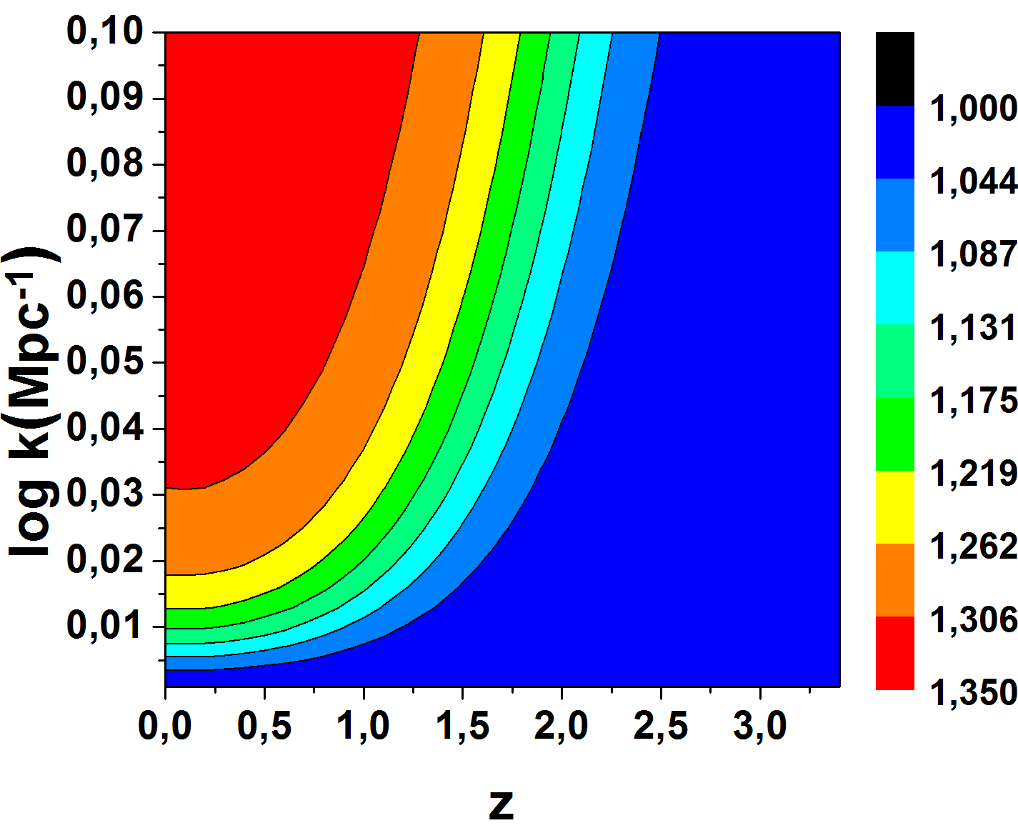
(a)   $G_{eff}/G$ (model I)

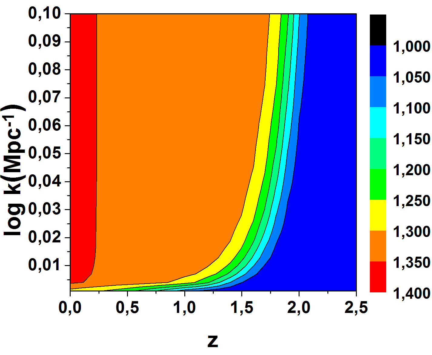
(b)   $G_{eff}/G$ (model II)

Figure 1: Contour plot of the effective gravitational constant $G_{\mathrm{eff}}/G$ as a function of $z$ and $\log k(\mathrm{Mpc}^{-1})$ for model I (a) and model II (b).

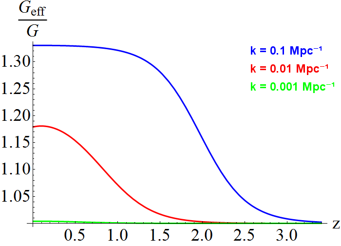
(a)   model I

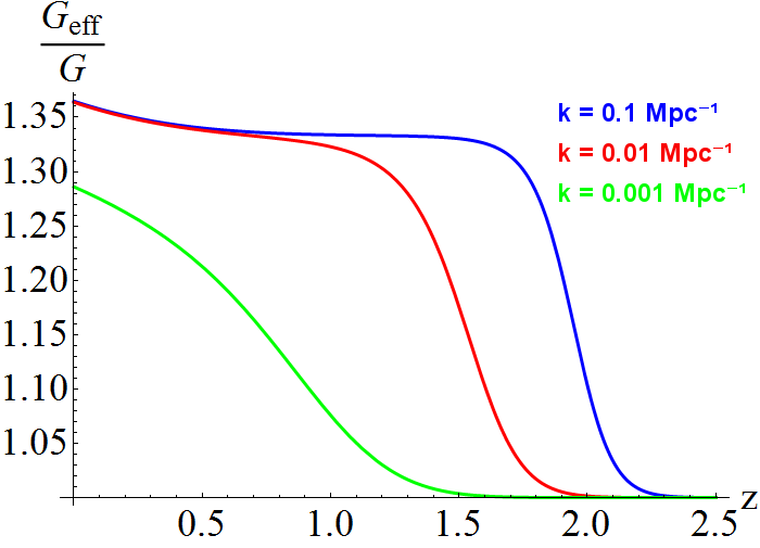
(b)   model II

Figure 2: Cosmological evolution of $G_{\mathrm{eff}}/G$ as a function of $z$ for $k=0.1\mathrm{Mpc}^{-1}$ (blue line), $k=0.01\mathrm{Mpc}^{-1}$ (red line) and $k=0.001\mathrm{Mpc}^{-1}$ (green line) for model I (a) and model II (b).

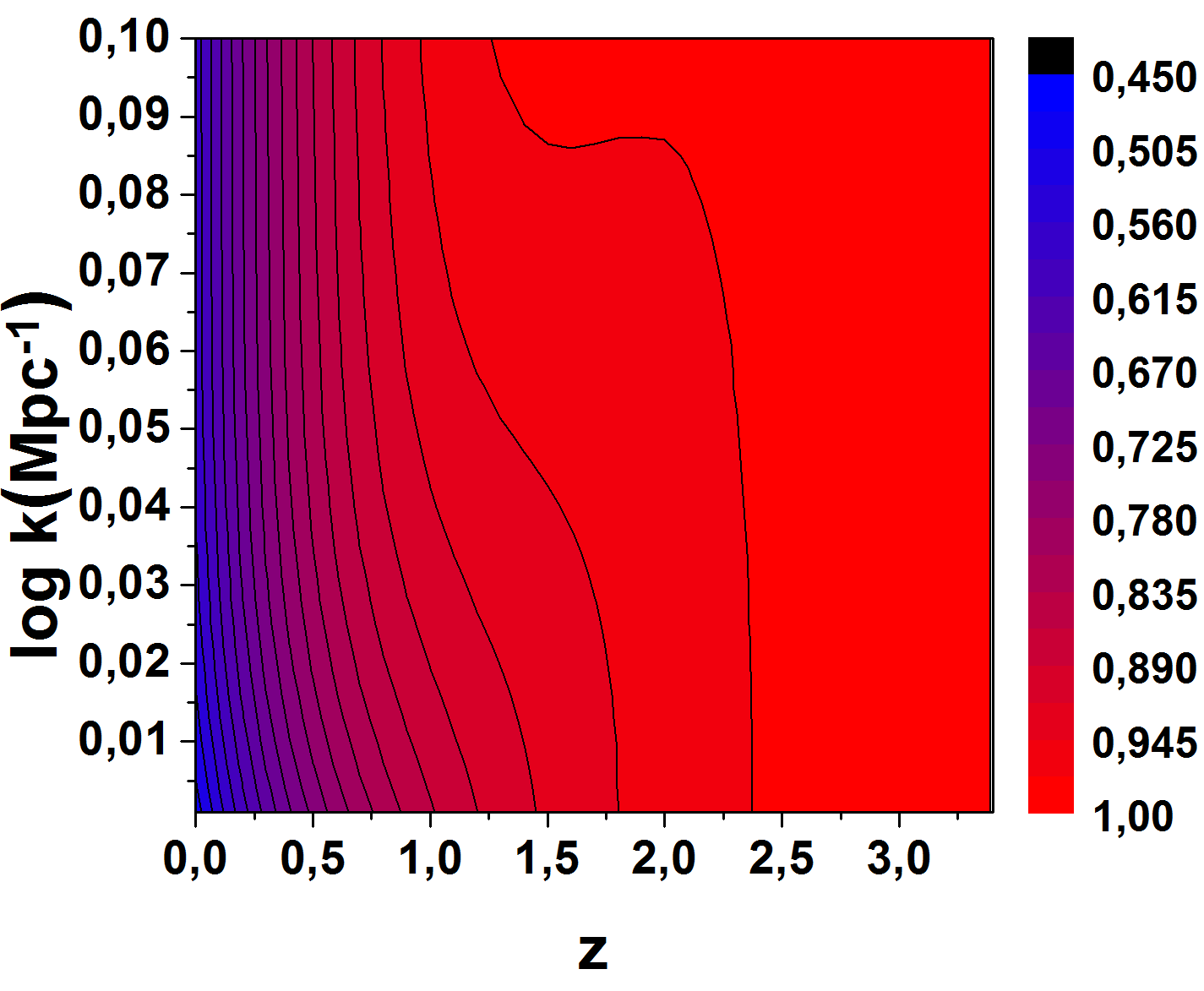
(a)   $f_{\mathrm{g}}$ (model I)

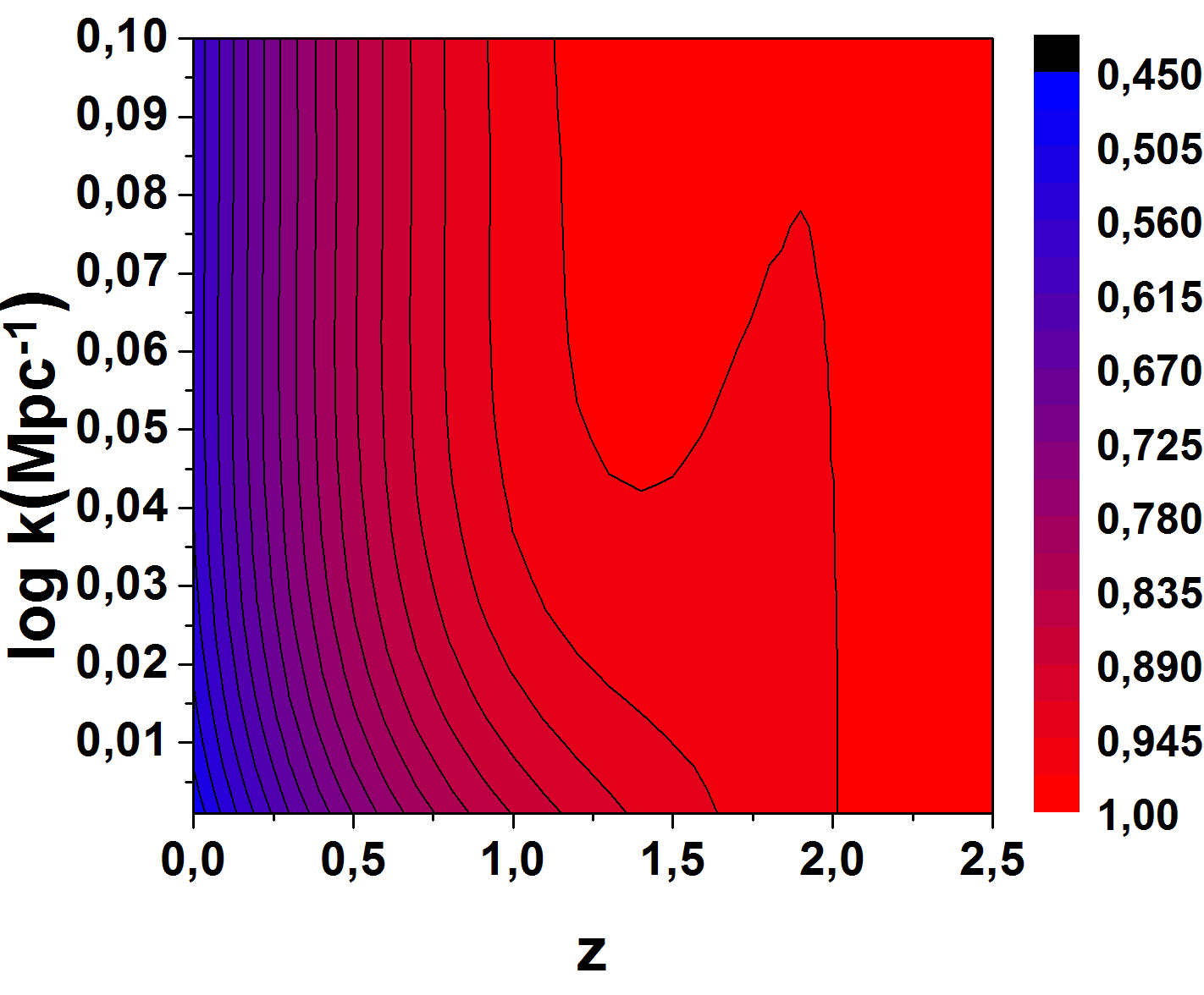
(b)   $f_{\mathrm{g}}$ (model II)

Figure 3: Contour plot of the growth rate $f_{\mathrm{g}}$ as a function of $z$ and $\log k(\mathrm{Mpc}^{-1})$ for model I (a) and model II (b).

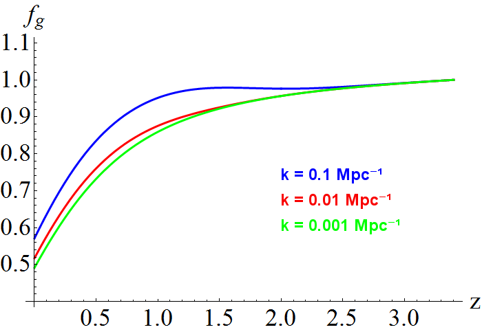
(a)   model I

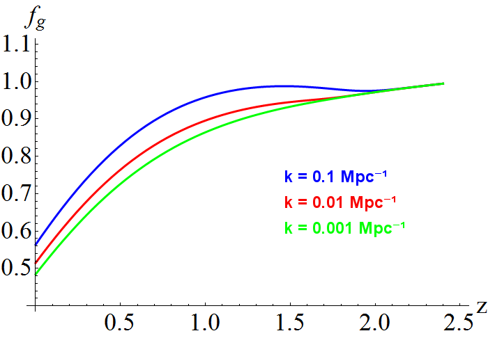
(b)   model II

Figure 4: Cosmological evolution of the growth rate $f_{\mathrm{g}}$ as a function of $z$ for $k=0.1\mathrm{Mpc}^{-1}$ (blue line), $k=0.01\mathrm{Mpc}^{-1}$ (red line) and $k=0.001\mathrm{Mpc}^{-1}$ (green line) for model I (a) and model II (b).

In Figs. 1 and 2, the cosmological evolution of the ratio $G_{eff}/G$ as a function of redshift $z$ and the comoving wave number $k$ for both model I and model II is depicted.

The appearance of the comoving wave number $k$ in the expression of the effective gravitational constant $G_{\mathrm{eff}}$ has a huge importance due to the fact that now the evolution of the matter density perturbations also depends on $k$. This kind of dependence does not appear in the framework of general relativity. This fact can be easily checked by taking $F(R)=R$ in Eq. (35).

In deriving Eq. (34), I assume the subhorizon approximation (see EspositoFarese:2000ij ), for which the comoving wavelengths $\lambda\equiv a/k$ are considered to be much shorter than the Hubble radius $H^{-1}$. In terms of the comoving wave number, the subhorizon approximation can be written as follows:

$$\frac{k^{2}}{a^{2}}\gg H^{2}\,.$$ (36)

For model I, the subhorizon approximation states that $k\gg 0.000116\mathrm{Mpc}^{-1}$. For model II, it states that $k\gg 0.000118\mathrm{Mpc}^{-1}$. In order to fulfill (36), the values considered for $k$ in this work will always satisfy $\log k\geq-3$, with $k$ written in $\mathrm{Mpc}^{-1}$, for both model I and model II. From now on, the expression $\log k(\mathrm{Mpc}^{-1})$ will be used to specify taking the logarithm of $k$, with $k$ written in $\mathrm{Mpc}^{-1}$. On the other hand, deviations from the linear regime have to be taken into account Cardone:2012xv when $\log k(\mathrm{Mpc}^{-1})>-1$. Thus, the range of values considered for $k$ throughout this work for both model I and model II is

$$-3\leq\log k(\mathrm{Mpc}^{-1})\leq-1\,.$$

Equation (34) can be written in a different way by using the so-called growth rate $f_{\mathrm{g}}$ given by $f_{\mathrm{g}}\equiv d\ln{\delta}/d\ln{a}$. In terms of this growth rate, Eq. (34) reduces to

$$\frac{df_{\mathrm{g}}(z)}{dz}\,+\,\left(\frac{1+z}{H(z)}\frac{dH(z)}{dz}-2-f_{\mathrm{g}}(z)\right)\frac{f_{\mathrm{g}}(z)}{1+z}+\frac{3}{2}\frac{\tilde{m}^{2}(1+z)^{2}}{H^{2}(z)}\frac{G_{\mathrm{eff}}(a(z),k)}{G}=0\,.$$ (37)

This equation can be solved numerically for model I and model II by imposing the condition that at high redshift the results for the $\Lambda$CDM universe are recovered. In Figs. 3 and 4, the growth rate is shown as a function of the redshift $z$ and the comoving wave number $k$ for model I and model II.

The next step should be to use the growth rate of these two models to compare them, but a new problem comes up when we face this task. Equation (37) usually must be solved numerically because of its complexity. This means that, generally, we will not have an analytic expression for the growth rate to deal with. In order to compare and discriminate among different theories it would be helpful to have one or more parameters that characterize their growth history.

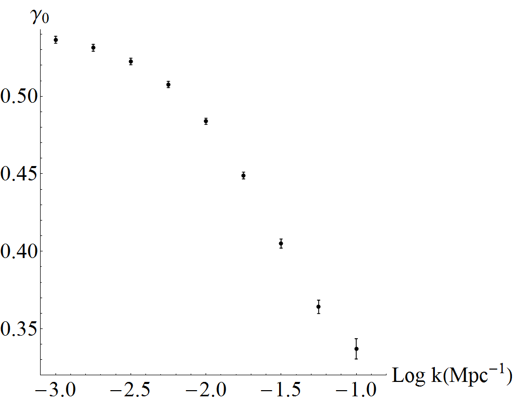
(a)  model I

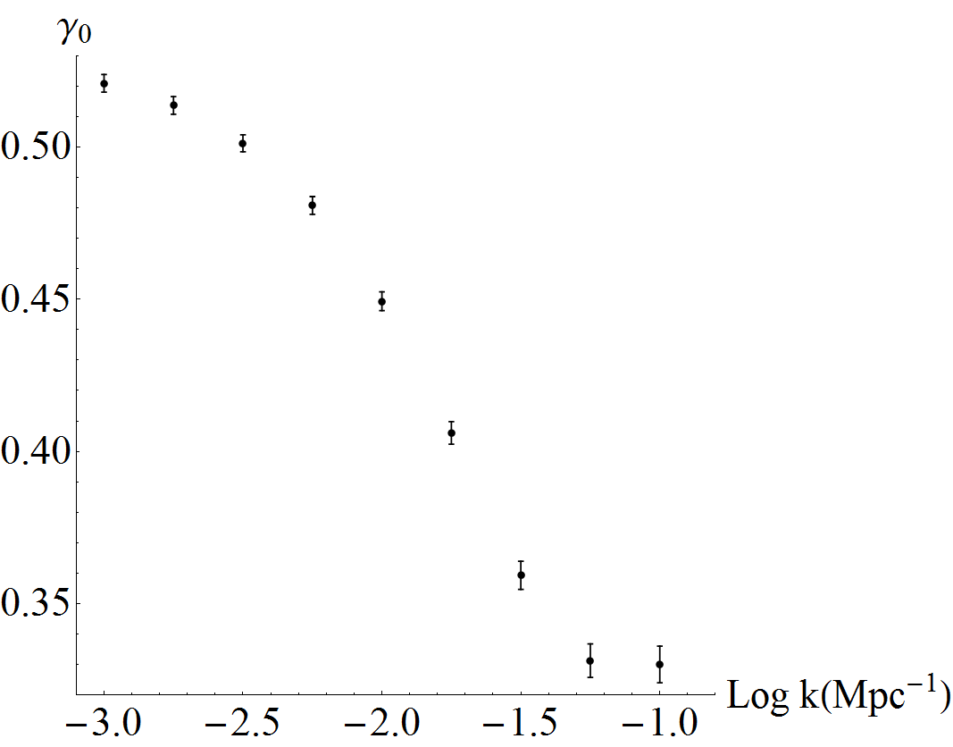
(b)  model II

Figure 5: Constant growth index as a function of $\log k(\mathrm{Mpc}^{-1})$ for model I (a) and for model II (b). The bars express the $68\%$ CL.

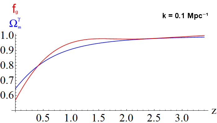
(a)  model I

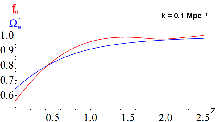
(b)  model II

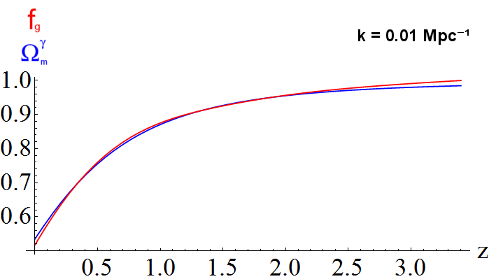
(c)  model I

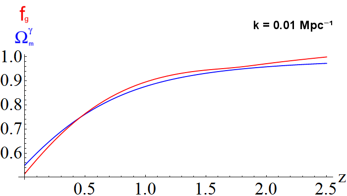
(d)  model II

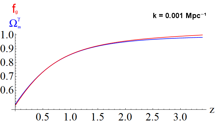
(e)  model I

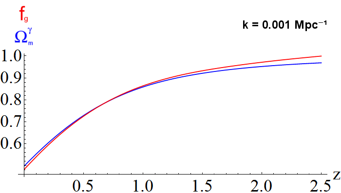
(f)  model II

Figure 6: Cosmological evolutions of the growth rate $f_{\mathrm{g}}$ (red line) and $\Omega_{\mathrm{m}}^{\gamma}$ (blue line) with $\gamma=\gamma_{0}$ as functions of the redshift $z$ in model I for $k=0.1\mathrm{Mpc}^{-1}$ (a), $k=0.01\mathrm{Mpc}^{-1}$ (c) and $k=0.001\mathrm{Mpc}^{-1}$ (e), and those in model II for $k=0.1\mathrm{Mpc}^{-1}$ (b), $k=0.01\mathrm{Mpc}^{-1}$ (d) and $k=0.001\mathrm{Mpc}^{-1}$ (f).

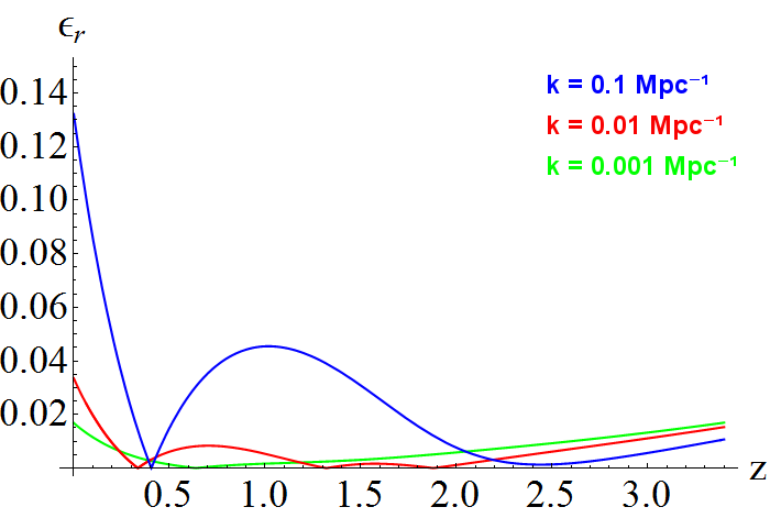
(a)  model I

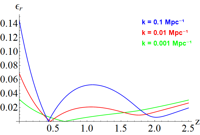
(b)  model II

Figure 7: Cosmological evolution of the relative difference $\epsilon_{r}=\frac{\left|f_{\mathrm{g}}-\Omega_{\mathrm{m}}^{\gamma}\right|}{f_{\mathrm{g}}}$ with $\gamma=\gamma_{0}$ for $k=0.1\mathrm{Mpc}^{-1}$ (blue line), $k=0.01\mathrm{Mpc}^{-1}$ (red line) and $k=0.001\mathrm{Mpc}^{-1}$ (green line) in model I (a) and model II (b).

V Characterizing the growth history: Growth index

In this section the concept of the growth index is developed. The growth index $\gamma$ appears as an important quantity in characterizing the growth of matter density perturbations.

In order to compare the growth of matter density perturbations between different theories, the so-called growth index $\gamma$ appears. This index is given by

$$f_{\mathrm{g}}(z)=\Omega_{\mathrm{m}}(z)^{\gamma(z)},$$ (38)

where $\Omega_{\mathrm{m}}(z)=\frac{8\pi G\rho_{m}}{3H^{2}}$ is the matter density parameter. The growth index $\gamma$ cannot be directly observed, but it could have a huge importance in discriminating among different gravitational theories; it can be inferred from the observational data of both the growth factor $f_{\mathrm{g}}(z)$ and the matter density parameter $\Omega_{\mathrm{m}}(z)$ at the same redshift $z$.

As it was done in Bamba:2012qi , different parametrizations for the growth index $\gamma$ will be considered for both model I and model II. In a first stage, a constant $\gamma$ will be assumed Kaiser:1987qv ; Hamilton:1997zq ; afterwards, a linear dependence Polarski:2007rr given by $\gamma(z)=\gamma_{0}+\gamma^{\prime}_{0}\cdot z$ will be considered; and, finally, an ansatz of the type $\gamma(z)=\gamma_{0}+\gamma_{1}\cdot z/(1+z)$ will be suggested.

In what follows, we will study these different parametrizations of the growth index for model I and model II.

V.1 $\gamma=\gamma_{0}$

We consider the ansatz for the growth index given by

$$\gamma=\gamma_{0},$$ (39)

where $\gamma_{0}$ is a constant.

The results obtained by fitting Eq. (38) to the solution of Eq. (37) for different values of the comoving wave number $k$ for model I and model II are shown in Fig. 5, where the points denote the median value while the bars express the $68\%$ confidence level (CL). It can be easily observed that both models exhibit a strong and quite similar dependence on $\log k(\mathrm{Mpc}^{-1})$. Moreover, $\gamma$ seems to be worse determined for model II.

The cosmological evolutions of the growth rate $f_{\mathrm{g}}(z)$ and the expression $\Omega_{\mathrm{m}}(z)^{\gamma_{0}}$ as functions of the redshift $z$ for several values of the comoving wave number $k$ for model I and model II are depicted in Fig. 6. From what is shown in this figure it is clear that the worst fit is given for the highest value of the comoving wave number $k$.

In order to clarify the results obtained, the relative difference between $f_{\mathrm{g}}(z)$ and $\Omega_{\mathrm{m}}(z)^{\gamma_{0}}$ is defined as

$$\epsilon_{r}(z,k)=\frac{\left|f_{\mathrm{g}}(z,k)-\Omega_{\mathrm{m}}(z)^{\gamma}\right|}{f_{\mathrm{g}}(z,k)}.$$ (40)

In Fig. 7, the cosmological evolution of $\epsilon_{r}$ as a function of $z$ for the same values of $k$ in both models are shown. For model I the relative difference is less than $13\%$ for $\log k(\mathrm{Mpc}^{-1})=-1$, $3.5\%$ for $\log k(\mathrm{Mpc}^{-1})=-2$ and $2\%$ for $\log k(\mathrm{Mpc}^{-1})=-3$; while for model II, the highest value of $\epsilon_{r}$ is $14\%$ for $\log k(\mathrm{Mpc}^{-1})=-1$, $7\%$ for $\log k(\mathrm{Mpc}^{-1})=-2$ and $3\%$ for $\log k(\mathrm{Mpc}^{-1})=-3$. Thus, two points can be made. First of all, the fits for model I are, generally, better than the ones for model II. Second of all, the fits are better for lower values of $\log k(\mathrm{Mpc}^{-1})$ for both models.

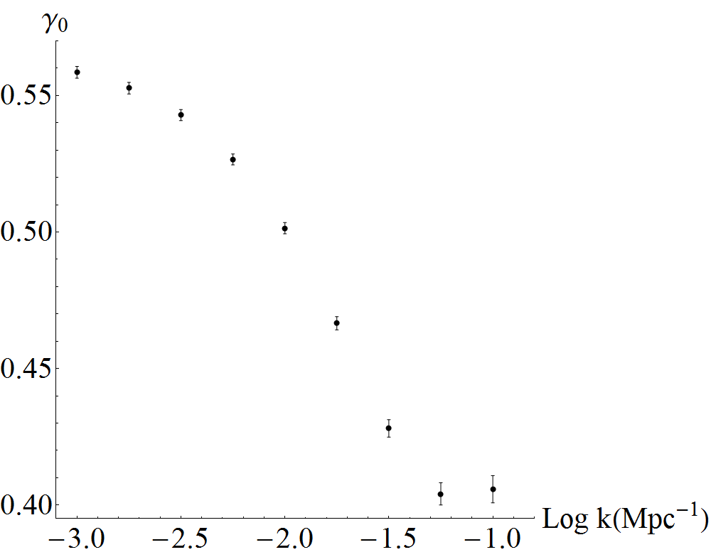
(a)  model I

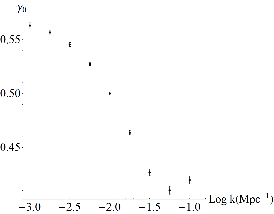
(b)  model II

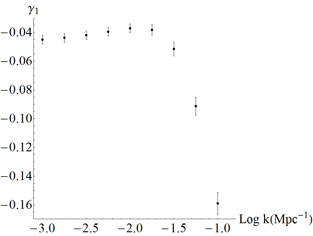
(c)  model I

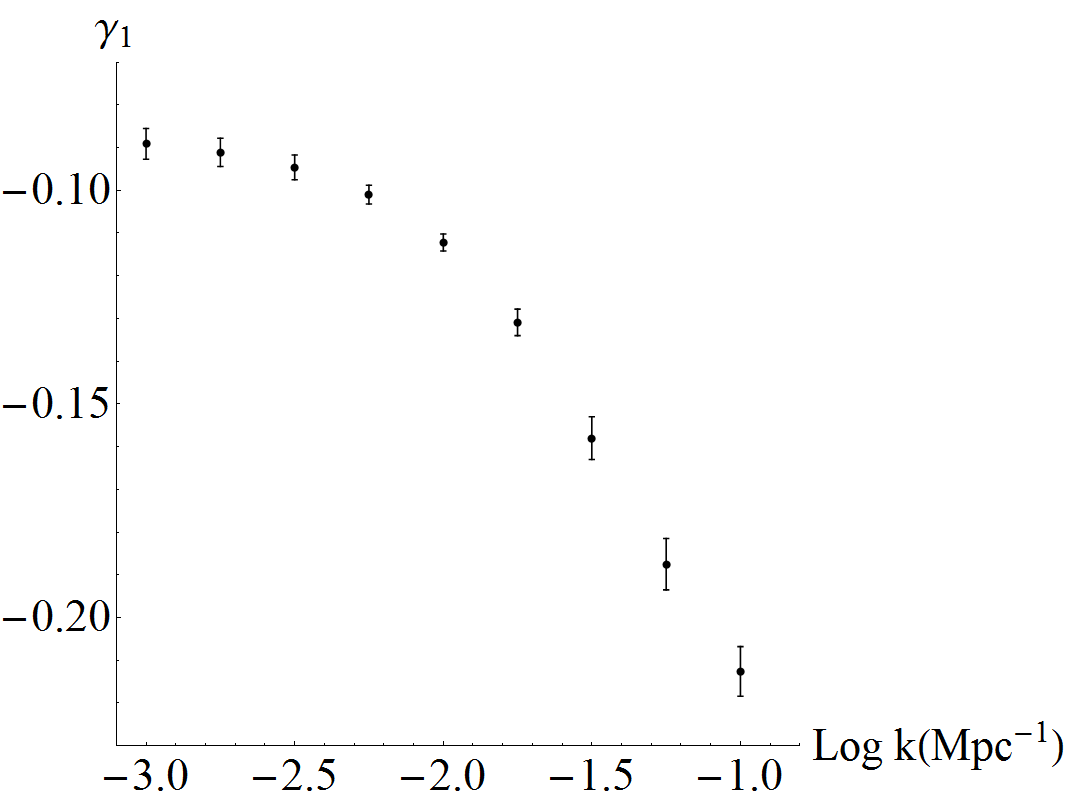
(d)  model II

Figure 8: Growth index fitting parameters in the case $\gamma=\gamma_{0}+\gamma_{1}\cdot z$ as a function of $\log k(\mathrm{Mpc}^{-1})$ for model I [(a) and (c)] and model II [(b) and (d)]. The legend is the same as Fig. 5.

V.2 $\gamma=\gamma_{0}+\gamma_{1}\cdot z$

In this subsection, the case of a growth index given by

$$\gamma=\gamma_{0}+\gamma_{1}\cdot z,$$ (41)

where $\gamma_{0}$ and $\gamma_{1}$ are constants, will be studied following the same steps taken in the case of a constant growth index. The results obtained with this ansatz should improve those for a constant growth index.

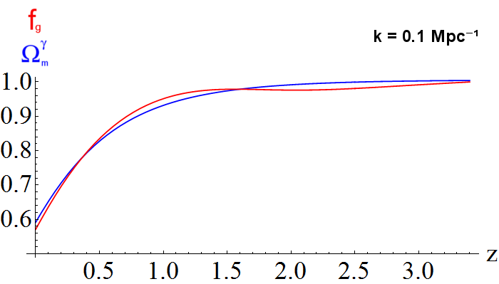
(a)  model I

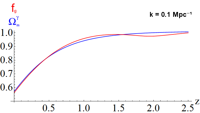
(b)  model II

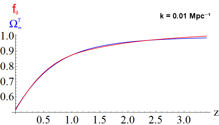
(c)  model I

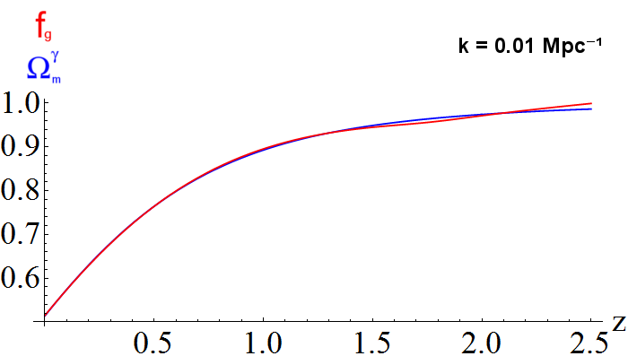
(d)  model II

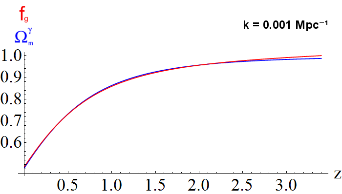
(e)  model I

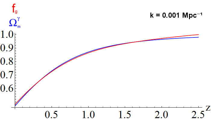
(f)  model II

Figure 9: Cosmological evolutions of the growth rate $f_{\mathrm{g}}$ (red line) and $\Omega_{\mathrm{m}}^{\gamma}$ (blue line) with $\gamma=\gamma_{0}+\gamma_{1}\cdot z$ as functions of the redshift $z$ in model I for $k=0.1\mathrm{Mpc}^{-1}$ (a), $k=0.01\mathrm{Mpc}^{-1}$ (c) and $k=0.001\mathrm{Mpc}^{-1}$ (e), and those in model II for $k=0.1\mathrm{Mpc}^{-1}$ (b), $k=0.01\mathrm{Mpc}^{-1}$ (d) and $k=0.001\mathrm{Mpc}^{-1}$ (f).

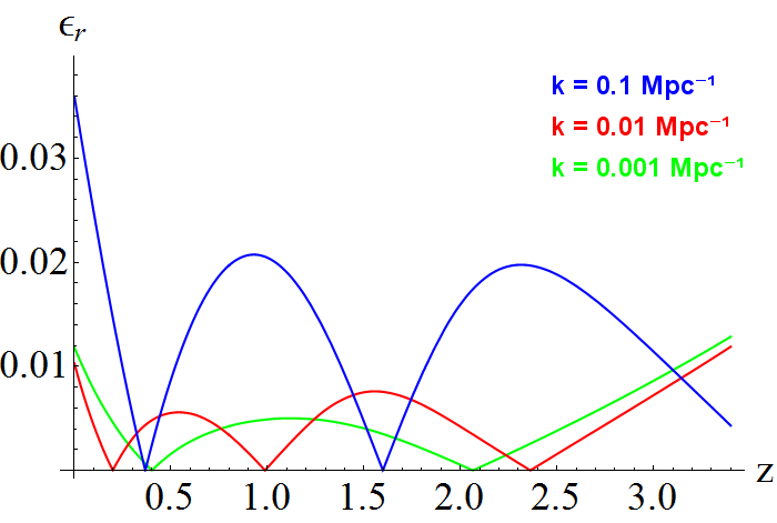
(a)  model I

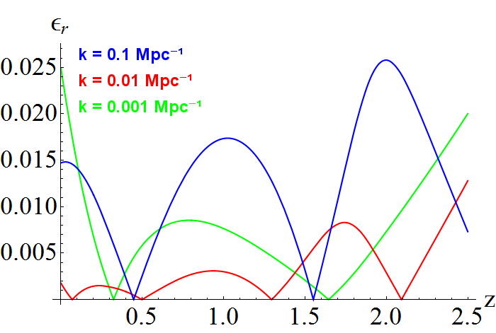
(b)  model II

Figure 10: Cosmological evolution of the relative difference $\epsilon_{r}=\frac{\left|f_{\mathrm{g}}-\Omega_{\mathrm{m}}^{\gamma}\right|}{f_{\mathrm{g}}}$ with $\gamma=\gamma_{0}+\gamma_{1}\cdot z$ for $k=0.1\mathrm{Mpc}^{-1}$ (blue line), $k=0.01\mathrm{Mpc}^{-1}$ (red line) and $k=0.001\mathrm{Mpc}^{-1}$ (green line) in model I (a) and model II (b).

In Fig. 8, the parameters $\gamma_{0}$ and $\gamma_{1}$ for several values of $\log k(\mathrm{Mpc}^{-1})$ in both models are shown. For model I, $\gamma_{0}$ exhibits a clear dependence on $\log k(\mathrm{Mpc}^{-1})$, while $\gamma_{1}$ is almost constant for $-3\leq\log k(\mathrm{Mpc}^{-1})\leq-1.75$. For model II, the dependence on $\log k(\mathrm{Mpc}^{-1})$ is strong for both $\gamma_{0}$ and $\gamma_{1}$ throughout the range of values considered for $\log k(\mathrm{Mpc}^{-1})$. It may also be noted that the parameter $\gamma_{1}$ gives the main difference between model I and model II.

In Fig. 9, the cosmological evolutions of the growth rate $f_{\mathrm{g}}(z)$ and $\Omega_{\mathrm{m}}(z)^{\gamma(z)}$ as functions of the redshift $z$ together for model I and model II are depicted. Compared with the fits for a constant growth index, it can be easily noticed that the linear ansatz improves the results obtained, especially in the case of $\log k(\mathrm{Mpc}^{-1})=-1$.

The cosmological evolution of the relative difference $\epsilon_{r}$ as a function of $z$ for several values of $k$ in model I and model II is shown in Fig. 10. For model I the relative difference is less than $3.5\%$ for $\log k(\mathrm{Mpc}^{-1})=-1$ and $1.5\%$ for $\log k(\mathrm{Mpc}^{-1})\leq-2$; while for model II, the highest value of $\epsilon_{r}$ is $2.5\%$ for $\log k(\mathrm{Mpc}^{-1})=-1$, $1.5\%$ for $\log k(\mathrm{Mpc}^{-1})=-2$ and $2.5\%$ for $\log k(\mathrm{Mpc}^{-1})=-3$. It might be accurate to note that these results improve those obtained for the case given by $\gamma=\gamma_{0}$, particulary those for the case $\log k(\mathrm{Mpc}^{-1})=-1$.

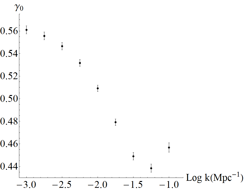
(a)  model I

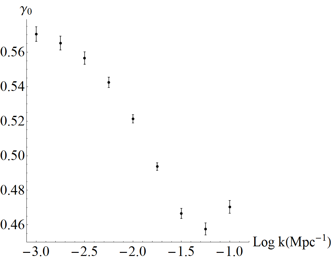
(b)  model II

(c)  model I

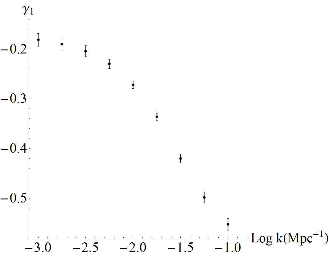
(d)  model II

Figure 11: Growth index fitting parameters in the case $\gamma=\gamma_{0}+\gamma_{1}\cdot\frac{z}{1+z}$ as a function of $\log k(\mathrm{Mpc}^{-1})$ for model I [(a) and (c)] and model II [(b) and (d)]. The legend is the same as Fig. 5.

V.3 $\gamma=\gamma_{0}+\gamma_{1}\cdot\frac{z}{1+z}$

Finally, we assume the following ansatz for the growth index:

$$\gamma=\gamma_{0}+\gamma_{1}\cdot\frac{z}{1+z},$$ (42)

where $\gamma_{0}$ and $\gamma_{1}$ are constants.

The parameters $\gamma_{0}$ and $\gamma_{1}$ for several values of $\log k$ are shown in Fig. 11 for both models. For model I, as it happened in the linear case, $\gamma_{0}$ exhibits a strong dependence on $\log k(\mathrm{Mpc}^{-1})$, while $\gamma_{1}$ is almost constant for $-3\leq\log k(\mathrm{Mpc}^{-1})\leq-2$. In the case of model II, the dependence on $\log k(\mathrm{Mpc}^{-1})$ is clear for both parameters $\gamma_{0}$ and $\gamma_{1}$.

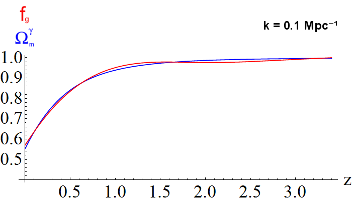
(a)  model I

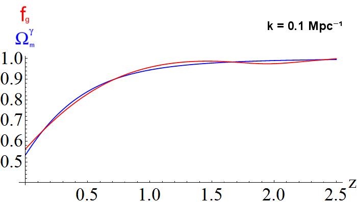
(b)  model II

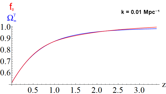
(c)  model I

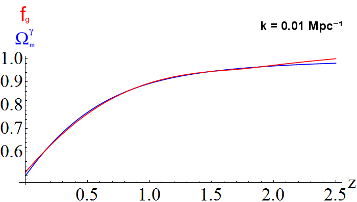
(d)  model II

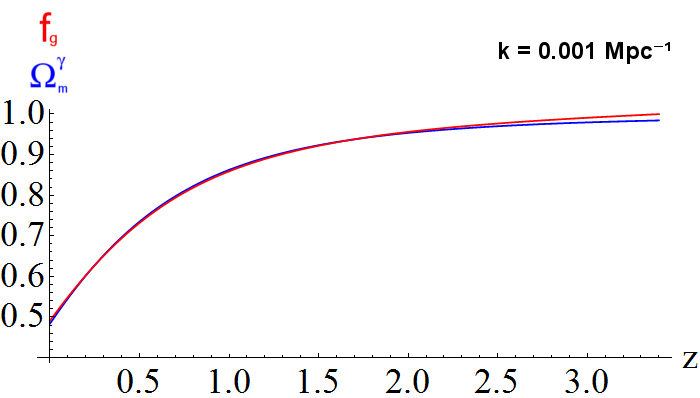
(e)  model I

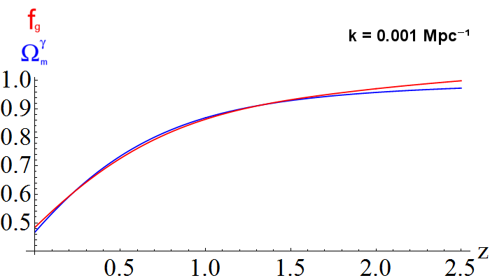
(f)  model II

Figure 12: Cosmological evolutions of the growth rate $f_{\mathrm{g}}$ (red line) and $\Omega_{\mathrm{m}}^{\gamma}$ (blue line) with $\gamma=\gamma_{0}+\gamma_{1}\cdot\frac{z}{1+z}$ as functions of the redshift $z$ in model I for $k=0.1\mathrm{Mpc}^{-1}$ (a), $k=0.01\mathrm{Mpc}^{-1}$ (c) and $k=0.001\mathrm{Mpc}^{-1}$ (e), and those in model II for $k=0.1\mathrm{Mpc}^{-1}$ (b), $k=0.01\mathrm{Mpc}^{-1}$ (d) and $k=0.001\mathrm{Mpc}^{-1}$ (f).

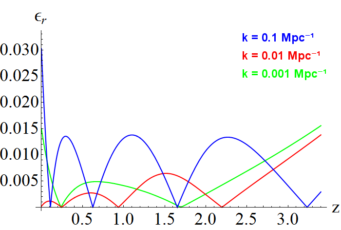
(a)  model I

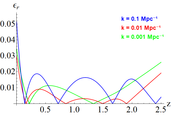
(b)  model II

Figure 13: Cosmological evolution of the relative difference $\epsilon_{r}=\frac{\left|f_{\mathrm{g}}-\Omega_{\mathrm{m}}^{\gamma}\right|}{f_{\mathrm{g}}}$ with $\gamma=\gamma_{0}+\gamma_{1}\cdot\frac{z}{1+z}$ for $k=0.1\mathrm{Mpc}^{-1}$ (blue line), $k=0.01\mathrm{Mpc}^{-1}$ (red line) and $k=0.001\mathrm{Mpc}^{-1}$ (green line) in model I (a) and model II (b).

The cosmological evolutions of the growth rate $f_{\mathrm{g}}(z)$ and $\Omega_{\mathrm{m}}(z)^{\gamma(z)}$ in model I and model II for several values of $k$ are depicted in Fig. 12. The fits in this case improve the results obtained for a constant growth index, but they seem similar to those obtained for the linear case.

As in the previous subsections, the relative difference $\epsilon_{r}$ for several values of $k$ in model I and model II is shown in Fig. 13 in order to analyze the fits quantitatively. For model I the relative difference is less than $3\%$ for $\log k(\mathrm{Mpc}^{-1})=-1$ and $1.5\%$ for $\log k(\mathrm{Mpc}^{-1})\leq-2$; while for model II, the highest value of $\epsilon_{r}$ is $5\%$ for $\log k(\mathrm{Mpc}^{-1})=-1$, $3\%$ for $\log k(\mathrm{Mpc}^{-1})=-2$ and $3.5\%$ for $\log k(\mathrm{Mpc}^{-1})=-3$. These results improve those obtained for the case given by $\gamma=\gamma_{0}$. For model I the results are very similar to the corresponding ones of $\gamma=\gamma_{0}+\gamma_{1}\cdot z$, but for model II they are worse.

To conclude, it is important to point out that three parametrizations for the growth index have been studied for both model I and model II. As it may have been expected, the fits obtained for a constant growth index give the worst results. The results obtained for the other two ansatz considered, i.e. $\gamma=\gamma_{0}+\gamma_{1}\cdot z$ and $\gamma=\gamma_{0}+\gamma_{1}\cdot\frac{z}{1+z}$, are quite similar for model I, but $\gamma=\gamma_{0}+\gamma_{1}\cdot z$ gives better fits for model II than those corresponding to the ansatz $\gamma=\gamma_{0}+\gamma_{1}\cdot\frac{z}{1+z}$. In conclusion, the linear ansatz, $\gamma=\gamma_{0}+\gamma_{1}\cdot z$, is the best parametrization for the growth index for the two models considered.

VI Discussion

In this section, the content of the paper is summarized and the results obtained for model I and model II are analyzed.

Two models of $F(R)$ modified gravity given by (26) and (31) have been considered throughout this work. The parameters of these models have been set in order to agree with current observational data coming from Komatsu:2010fb . Model (26) with the set of parameters given by (27) is the so-called model I, while model (31) with the set of parameters given by (32) is the so-called model II.

The growth of matter density perturbations has been studied for model I and model II. The so-called growth rate has been obtained numerically for both models and three ansatz for the so-called growth index have been considered. In Figs. 5, 8 and 11, the results of the different parametrizations for the growth index are shown for both models.

To determine which ansatz of those considered for the growth index fits better Eq. (38) to the solution of Eq. (37), the results obtained for the three parametrizations have been analyzed in the previous section. The ansatz given by $\gamma=\gamma_{0}+\gamma_{1}\cdot z$ seems to be the best choice for both models.

Thus, in order to discriminate between model I and model II (or with the models considered in Bamba:2012qi ) using the growth history, the values of $\gamma_{0}$ and $\gamma_{1}$ in $\gamma=\gamma_{0}+\gamma_{1}\cdot z$ could have an essential importance. In Fig. 14 these two parameters, $\gamma_{0}$ and $\gamma_{1}$, are depicted for the two models together. We see that the behavior of $\gamma_{0}$ is very similar for both models. However, the values for $\gamma_{1}$ are totally different for model I to model II and they could be used to discriminate between these two models.

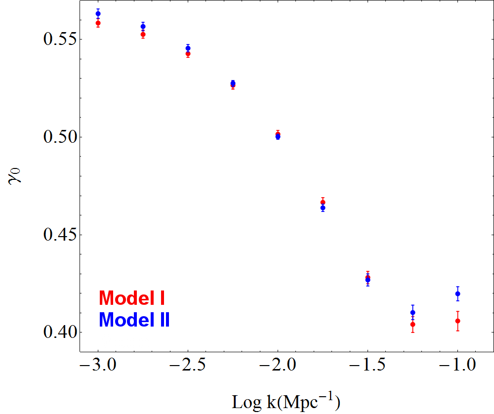
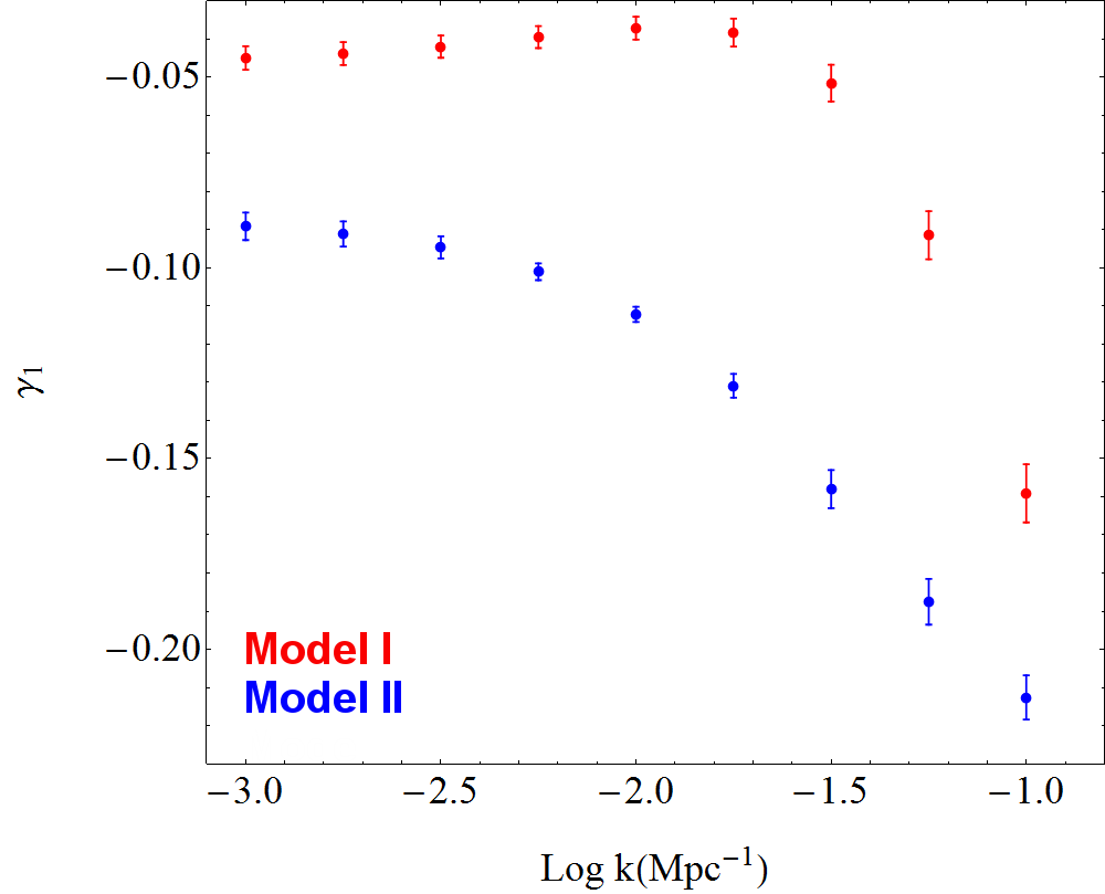
Figure 14: Growth index fitting parameters in the case $\gamma=\gamma_{0}+\gamma_{1}\cdot z$ as a function of $\log k(\mathrm{Mpc}^{-1})$. The legend is the same as Fig. 5.

One final note must be made. As it was pointed out in Eq.(34), the evolution of matter density perturbations for $F(R)$ modified gravity theories depends on the comoving wave number $k$, which does not occur in the framework of general relativity. Throughout this work, this fact has been confirmed, in the first place with the results obtained for the growth rate $f_{\mathrm{g}}$, and finally, with those obtained for each of the three parametrizations considered for the growth index $\gamma$. Nevertheless, these parametrizations do not depend on the comoving wave number $k$, and it may be very interesting in the future to propose some scale-dependent ansatz for these $F(R)$ modified gravity theories.

References

- (1) S. Perlmutter et al. [SNCP Collaboration], Astrophys. J. 517, 565 (1999) [arXiv:astro-ph/9812133]; A. G. Riess et al. [Supernova Search Team Collaboration], Astron. J. 116, 1009 (1998) [arXiv:astro-ph/9805201].
- (2) M. Tegmark et al. [SDSS Collaboration], Phys. Rev. D 69, 103501 (2004) [arXiv:astro-ph/0310723]; U. Seljak et al. [SDSS Collaboration], Phys. Rev. D 71, 103515 (2005) [arXiv:astro-ph/0407372].
- (3) D. J. Eisenstein et al. [SDSS Collaboration], Astrophys. J. 633, 560 (2005) [arXiv:astro-ph/0501171].
- (4) D. N. Spergel et al. [WMAP Collaboration], Astrophys. J. Suppl. 148, 175 (2003) [arXiv:astro-ph/0302209]; Astrophys. J. Suppl. 170, 377 (2007) [arXiv:astro-ph/0603449].
- (5) E. Komatsu et al. [WMAP Collaboration], Astrophys. J. Suppl. 180, 330 (2009) [arXiv:0803.0547 [astro-ph]].
- (6) E. Komatsu et al. [WMAP Collaboration], Astrophys. J. Suppl. 192 (2011) 18 [arXiv:1001.4538 [astro-ph.CO]].
- (7) B. Jain and A. Taylor, Phys. Rev. Lett. 91, 141302 (2003) [arXiv:astro-ph/0306046].
- (8) M. Li, X. D. Li, S. Wang and Y. Wang, Commun. Theor. Phys. 56, 525 (2011) [arXiv:1103.5870 [astro-ph.CO]].
- (9) M. Kunz, arXiv:1204.5482 [astro-ph.CO].
- (10) K. Bamba, S. Capozziello, S. Nojiri and S. D. Odintsov, arXiv:1205.3421 [gr-qc].
- (11) S. Nojiri and S. D. Odintsov, Phys. Rept. 505, 59 (2011) [arXiv:1011.0544 [gr-qc]]; eConf C0602061, 06 (2006) [Int. J. Geom. Meth. Mod. Phys. 4, 115 (2007)] [arXiv:hep-th/0601213].
- (12) S. Capozziello and V. Faraoni, Beyond Einstein Gravity: A Survey of Gravitational Theories for Cosmology and Astrophysics (Springer, Berlin, 2010).
- (13) T. Clifton, P. G. Ferreira, A. Padilla and C. Skordis, Phys. Rept. 513, 1 (2012) [arXiv:1106.2476 [astro-ph.CO]].
- (14) S. Capozziello and M. De Laurentis, Phys. Rept. 509, 167 (2011) [arXiv:1108.6266 [gr-qc]].
- (15) S. Capozziello, M. De Laurentis and S. D. Odintsov, arXiv:1206.4842 [gr-qc].
- (16) S. Nojiri and S. D. Odintsov, Phys. Lett. B 657 (2007) 238 [arXiv:0707.1941 [hep-th]]; S. Nojiri and S. D. Odintsov, Phys. Rev. D 77 (2008) 026007 [arXiv:0710.1738 [hep-th]], G. Cognola, E. Elizalde, S. Nojiri, S. D. Odintsov, L. Sebastiani and S. Zerbini, Phys. Rev. D 77 (2008) 046009 [arXiv:0712.4017 [hep-th]].
- (17) S. Nojiri and S. D. Odintsov, Phys. Rev. D 68 (2003) 123512 [hep-th/0307288];
- (18) T. Chiba, Phys. Lett. B 575, 1 (2003) [arXiv:astro-ph/0307338].
- (19) T. Chiba, T. L. Smith and A. L. Erickcek, Phys. Rev. D 75, 124014 (2007) [arXiv:astro-ph/0611867]; G. J. Olmo, Phys. Rev. D 75, 023511 (2007) [gr-qc/0612047].
- (20) A. D. Dolgov and M. Kawasaki, Phys. Lett. B 573, 1 (2003) [arXiv:astro-ph/0307285]; V. Faraoni, Phys. Rev. D 74, 104017 (2006) [arXiv:astro-ph/0610734].
- (21) Y. S. Song, W. Hu and I. Sawicki, Phys. Rev. D 75, 044004 (2007) [arXiv:astro-ph/0610532].
- (22) V. Muller, H. J. Schmidt and A. A. Starobinsky, Phys. Lett. B 202, 198 (1988); V. Faraoni and S. Nadeau, Phys. Rev. D 72, 124005 (2005) [arXiv:gr-qc/0511094].
- (23) G. Cognola, E. Elizalde, S. D. Odintsov, P. Tretyakov and S. Zerbini, Phys. Rev. D 79 (2009) 044001 [arXiv:0810.4989 [gr-qc]].
- (24) A. de la Cruz-Dombriz, A. Dobado, and A. L. Maroto, Phys. Rev. D 77, 123515 (2008); L. Pogosian, and A. Silvestri, Phys. Rev. D 77, 023503 (2008); idem, Phys. Rev. D 81, 049901(E) (2010); H. Oyaizu, Phys. Rev. D 78, 123523 (2008); H. Oyaizu, M. Lima, and W. Hu, Phys. Rev. D 78, 123524 (2008); F. Schmidt, M. Lima, H. Oyaizu, and W. Hu, Phys. Rev. D 79, 083518 (2009); G. B. Zhao, B. Li, and K. Koyama, Phys. Rev. D 83, 044007 (2011); K. Koyama, A. Taruya, and T. Hiramatsu, Phys. Rev. D 79, 123512 (2009); A. Taruya, T. Nishimichi, S. Saito, and T. Hiramatsu, Phys. Rev. D 80, 123503 (2009); F. Schmidt, Phys. Rev. D 78, 043002 (2008); G. B. Zhao, L. Pogosian, A. Silvestri, and J. Zylberberg, Phys. Rev. D 79, 083513 (2009); F. Schmidt, A. Vikhlinin, and W. Hu, Phys. Rev. D 80, 083505 (2009); A. Borisov, and B. Jain, Phys. Rev. D 79, 103506 (2009); S. Ferraro, F. Schmidt, W. Hu, Phys. Rev. D 83, 063503 (2011); K. W. Masui, F. Schmidt,, U. L. Pen, and P. McDonald, Phys. Rev. D 81, 062001 (2011); T. Giannantonio, M. Martinelli, A. Silvestri, and A. Melchiorri, JCAP 04, 030 (2010); K. Yamamoto, G. Nakamura, G. Hutsi, T. Narikawa, and T. Sato, Phys. Rev. D 81, 103517 (2010); E. Beynon, D. J. Bacon, and K. Koyama, Mon. Not. Roy. Astron. Soc. 403, 353 (2010); A. M. Nzioki, P. K. S. Dunsby, R. Goswami, and S. Carloni, Phys. Rev. D 83, 024030 (2011); X. Fu, P. Wu, and H. Yu, Eur. Phys. J. C 68, 271 (2010); T. Narikawa, and K. Yamamoto, Phys. Rev. D 81, 043528 (2010); ibidem, Phys. Rev. D 81, 129903(E) (2010); S. A. Thomas, S. A. Appleby, and J. Weller, JCAP 03, 036 (2011); L. Lombriser, F. Schmidt, T. Baldauf, R. Mandelbaum, U. Seljak, and R. E. Smith, arXiv:1111.2020; S. Camera, A. Diaferio, and V. F. Cardone, JCAP 07, 016 (2011)
- (25) E. V. Linder, Phys. Rev. D 72, 043529 (2005) [astro-ph/0507263].
- (26) S. Capozziello, S. Nojiri and S. D. Odintsov, Phys. Lett. B634, 93 (2006), hep-th/0512118; S. Capozziello, S. Nojiri, S. D. Odintsov and A. Troisi, Phys. Lett. B639, 135 (2006), astro-ph/0604431.
- (27) K. Bamba, A. Lopez-Revelles, R. Myrzakulov, S. D. Odintsov and L. Sebastiani, arXiv:1207.1009 [gr-qc].
- (28) S. Nojiri and S. D. Odintsov, Phys. Rev. D 77 (2008) 026007 [arXiv:0710.1738 [hep-th]].
- (29) W. Hu and I. Sawicki, Phys. Rev. D 76 (2007) 064004 [arXiv:0705.1158 [astro-ph]].
- (30) S. Nojiri and S. D. Odintsov, Prog. Theor. Phys. Suppl. 190 (2011) 155 [arXiv:1008.4275 [hep-th]].
- (31) S. Tsujikawa, Phys. Rev. D 76 (2007) 023514 [arXiv:0705.1032 [astro-ph]].
- (32) G. Esposito-Farese and D. Polarski, Phys. Rev. D 63 (2001) 063504 [arXiv:gr-qc/0009034].
- (33) V. F. Cardone, S. Camera and A. Diaferio, JCAP 1202 (2012) 030 [arXiv:1201.3272 [astro-ph]].
- (34) N. Kaiser, Mon. Not. Roy. Astron. Soc. 227 (1987) 1.
- (35) A. J. S. Hamilton, astro-ph/9708102.
- (36) D. Polarski and R. Gannouji, Phys. Lett. B 660 (2008) 439 [arXiv:0710.1510 [astro-ph]].