Lifshitz phase transitions in the ferromagnetic regime of the Kondo lattice model

Abstract

We establish the low-temperature phase diagrams of the spin-$1/2$ and spin-$1$ Kondo lattice models as a function of the conduction-band filling $n$ and the exchange coupling strength $J$ in the regime of ferromagnetic effective exchange interactions ($n\lesssim 0.5$). We show that both models have several distinct ferromagnetic phases separated by continuous Lifshitz transitions of the Fermi-pocket vanishing or emergence type: one of the phases has a true gap in the minority band (half metal), the others only a pseudogap. They can be experimentally distinguished by their magnetization curves; only the gapped phase exhibits magnetization rigidity. We find that, quite generically, ferromagnetism and Kondo screening coexist rather than compete, both in spin-$1/2$ and spin-$1$ models. We compute the Curie temperatures and establish a “ferromagnetic Doniach diagram” for both models.

Materials with competing interactions, such as many lanthanide and actinide compounds, have complex low-temperature phase diagrams with different ground states Coleman and Schofield (2005); Löhneysen et al. (2007); Si and Steglich (2010); Stewart (2001); Gegenwart et al. (2008); Pfleiderer (2009). The Kondo lattice model (KLM) Tsunetsugu et al. (1997); Gulácsi (2004); Hewson (1993) describes a conduction band of itinerant electrons and a lattice of local moments on $f$ shells, coupled at each site by an antiferromagnetic exchange interaction $J$. For large $J$, the moments are screened. The resulting paramagnetic state has Fermi liquid properties with strongly renormalized parameters. For small $J$, the conduction-band electrons are carriers of long-range magnetic interactions and the moments order. The two regimes are separated by a quantum phase transition at critical $J^{*}$, as described by the Doniach diagram Doniach (1977). The Néel temperature increases at first quadratically with $J$, but then it peaks and decreases to zero at $J^{*}$ as the Kondo screening takes over. The simplest version of the KLM with spin-$1/2$ moments indeed has an antiferromagnetic (AFM) ground state (Néel order) for small $J$ near half-filling Capponi and Assaad (2001); Otsuki et al. (2009a). The nature of the phase transition at $J^{*}$ has been investigated using a variety of methods, the most accurate of which confirm that the transition is second order (quantum critical) and indicate that it involves a change of the Fermi surface topology De Leo et al. (2008); Martin and Assaad (2008); Martin et al. (2010). In the spin-$1$ KLM, there is no phase transition at half-filling and the AFM phase extends to large values of $J$.

While most cerium compounds show AFM order, some are ferromagnetic (FM): CeRu₂Ge₂ Süllow et al. (1999), CeIn₂ Rojas et al. (2009); Mukherjee et al. (2012), and CeRu₂Al₂B Baumbach et al. (2012). A number of uranium and neptunium heavy-fermion materials are also FM: UTe Schoenes et al. (1984), UCu_0.9Sb₂ Bukowski et al. (2005), UCo_0.5Sb₂ Tran et al. (2005), NpNiSi₂ Colineau et al. (2008), Np₂PdGa₃ Tran et al. (2010), and UCu₂Si₂ Troć et al. (2012). In addition, there are strong indications of robust coexistence of the Kondo effect and ferromagnetism, in particular in U compounds. In Refs. Perkins et al. (2007a, b); Coqblin et al. (2009); Thomas et al. (2011); Troć et al. (2012) it has been proposed that an appropriate minimal model for this behavior is the spin-$1$ version of the KLM, where in the mean-field picture the conduction-band electrons underscreen the local moments, while the residual moments order ferromagnetically. FM order appears for low and moderate electron filling $n$ in the conduction band, $n\lesssim 0.5$ Lacroix and Cyrot (1979); Batista et al. (2002); Perkins et al. (2007a); Peters and Pruschke (2007); Otsuki et al. (2009b). Mean-field analysis predicts two phases: for small $J$ the stable phase is a FM regular metal, while for large $J$ there is a transition to a FM heavy metal. Dynamical mean-field theory (DMFT) calculations demonstrated that the spin-$1/2$ KLM also has a FM order coexisting with (incomplete) Kondo screening Peters et al. (2012). Furthermore, this phase is a half-metal with gapped minority-spin band and a commensurability condition relates the magnetization to filling $n$ Peters et al. (2012) due to completely filled minority-spin lower band Beach and Assaad (2008); Viola Kusminskiy et al. (2008). A recent mean-field analysis of the spin-$1/2$ model suggested the presence of several different ferromagnetic phases Liu et al. (2013). So far, however, a single FM phase has been identified in the DMFT calculations Peters and Pruschke (2007); Otsuki et al. (2009b).

These findings open a number of questions: What is the relationship between ferromagnetism and Kondo screening: do they compete or coexist? What is the minimal model for studying these effects, spin-$1/2$ or spin-$1$ KLM? Is there a quantum phase transition between different FM states also in the spin-$1/2$ model? What is the nature of these transitions and what are their experimental signatures? And, finally, which aspects of the static mean-field analysis mf are correct and which must be revised in more accurate dynamical treatment? To answer these questions we have performed extensive DMFT Georges et al. (1996) calculations using the numerical renormalization group (NRG) as the impurity solver Wilson (1975); Bulla et al. (2008); Hofstetter (2000); Peters et al. (2006); Weichselbaum and von Delft (2007); Žitko and Pruschke (2009), as well as static mean-field calculations for both models mf .

We consider the Kondo lattice model

$$\begin{split}\mathcal{H}&=\sum_{{\mathbf{k}}\sigma}(\epsilon_{k}-\mu)c^{\dagger}_{{\mathbf{k}}\sigma}c_{{\mathbf{k}}\sigma}+J\sum_{i}{\mathbf{s}}_{i}\cdot{\mathbf{S}}_{i},\\ \end{split}$$ (1)

which describes a single-orbital conduction band with dispersion $\omega=\epsilon_{k}$, and a lattice of local moments described by the spin-$S$ operators ${\mathbf{S}}_{i}$; ${\mathbf{s}}_{i}$ is the conduction-band spin-density at site $i$, and $J$ is the antiferromagnetic Kondo exchange coupling ($J>0$). We focus on the Bethe lattice that has a semicircular density of states with bandwidth $2D$.

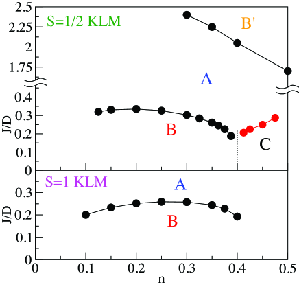
Figure 1: (Color online) Phase diagrams of spin-$1/2$ and spin-$1$ Kondo lattice models for $n<0.5$. Phase A is a ferromagnetic half-metal phase with strong Kondo effect where the minority band is gapped. Phases B and B’ are itinerant ferromagnetic phases with a pseudogap. Phase C for spin-1/2 model indicates the region with charge order Peters et al. (2013). For very small $n$, the calculations fail to converge.

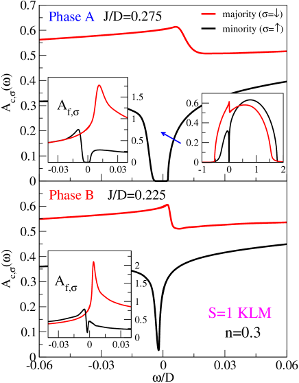
Figure 2: (Color online) Spin-resolved conduction-band local spectral functions $A_{c,\sigma}$ for the spin-$1$ KLM in the ferromagnetic half-metal phase (A) and in the itinerant ferromagnetic phase (B). The arrow indicates the main effect of decreasing interaction $J$: the lower edge of the upper hybridized band shifts to lower frequencies. The left insets in both panels show the $f$-level spectral functions $A_{f,\sigma}$ defined through the imaginary part of the scattering $T$ matrix. The right inset in the upper panel shows the spectral functions in the full frequency interval.

In Fig. 1 we present the main result of this work: the phase diagrams of the spin-$1/2$ and spin-$1$ KLM as a function of $n$ and $J$. For both spins we find several different ferromagnetic phases. Phase A corresponds to the ferromagnetic half-metal phase described by Peters et al. Peters et al. (2012). The corresponding spin-resolved spectral functions for the $S=1$ model are shown in Fig. 2, panel A. The minority spin band is gapped Peters et al. (2012), while the majority band exhibits the weak hybridization pseudo-gap characteristic of the Kondo lattice systems Pruschke et al. (2000); Costi and Manini (2002). Phase B at small $J$ is not gapped, but there is a pronounced pseudogap just below the Fermi level in the minority band, Fig. 2, panel B. The spectral functions for the $S=1/2$ model are qualitatively the same. The spectra thus suggest the occurrence of a Lifshitz transition at $J^{*}$: there is no change in the symmetry, but the Fermi surface of the minority band shrinks to a point and disappears as one goes from phase $B$ to $A$. We emphasize that the two phases exist both for spin-$1/2$ and for spin-$1$ models and have similar properties; clearly, within the DMFT, the value of the spin does not play a crucial role in the BA transition. $J^{*}$ is a non-monotonic function of $n$ that peaks at $n\sim 0.2$ and $n\sim 0.25$, respectively. Near $n\sim 0.4$ we observe change of behavior in the small-$J$ phase. For $S=1/2$ KLM, this is the parameter regime where charge order occurs Otsuki et al. (2009b); Peters et al. (2013), but it is not allowed for in our calculations.

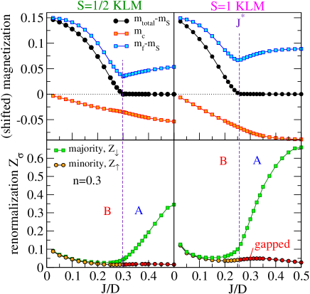
Figure 3: (Color online) Total, conduction-band $c$-level and localized $f$-level magnetizations (top panels) and the spin-dependent quasiparticle renormalization factors $Z_{\sigma}$ (bottom panels) across the phase transition, indicated by the vertical dashed lines. The magnetization is here defined as the expectation value of the spin operator: $m_{f}=\langle S_{z}\rangle$, $m_{c}=(n_{\uparrow}-n_{\downarrow})/2$, $m_{\mathrm{total}}=m_{f}+m_{c}$. In the plots, $m_{\mathrm{total}}$ and $m_{f}$ are shifted by $m_{S}$ defined in Eq. (2).

In Fig. 3 we plot the magnetization and the quasiparticle renormalization factor $Z_{\sigma}=[1-\mathrm{d}\Sigma_{\sigma}/\mathrm{d}\omega(\omega=\mu)]^{-1}$ as a function of $J$ across the BA transition. The frozen magnetization in phase A is given by a generalization of the spin-$1/2$ KLM result from Refs. Beach and Assaad (2008); Viola Kusminskiy et al. (2008); Peters et al. (2012):

$$m_{S}=(2S-n)/2.$$ (2)

At transition, the magnetization is continuous with a change of slope in $m_{f}$. This is in disagreement with the static mean-field analysis for $S=1$ which predicts a jump Perkins et al. (2007b). The factors $Z_{\sigma}$ for both spin orientations are continuous and finite across the transition (in the minority band of phase A there are no quasiparticles, but $Z_{\sigma}$ can formally still be defined). There is thus no criticality in this spin-selective metal-insulator transition, which may be identified as a continuous Lifshitz transition of the Fermi pocket vanishing type Lifshitz (1960); Yamaji et al. (2006); Viola Kusminskiy et al. (2008); Beach and Assaad (2008); Li et al. (2010); Bercx and Assaad (2012). The Fermi surface topology is continuous with no reorganization. Deep in the phase A, the majority electrons become weakly correlated ($Z$ has a value of order $0.5$).

For very large $J$, in the spin-$1/2$ model (but not for spin-$1$) there is another Lifshitz transition to a non-gapped phase Peters that we denote as B’. While in the BA transition, the chemical potential is located at the bottom of the upper hybridized band, in the AB’ transition the chemical potential is located at the top of the lower hybridized band at the transition point. In other words, while BA corresponds to the vanishing of electron pocket, AB’ corresponds to the emergence of hole pocket. For even larger $J$, the system eventually becomes paramagnetic (for $n=0.3$ at $J/D=3.4$).

The static mean-field theory for $S=1/2$ also predicts distinct phases Liu et al. (2013); mf which roughly correspond to B, A, and B’. The exact treatment of quantum fluctuations in DMFT leads, however, to a number of differences: i) The small-$J$ phase B is not pure ferromagnetic, but there is a coexistence with the Kondo effect. In the static MF treatment only pure ferromagnetic solution is stable and the phase transition from the corresponding phases A to B is of the first order Li et al. (2010), for details see Supplementary materials mf . Small-$J$ phase B is not pure ferromagnetic. ii) The Lifshitz transitions are all continuous: there are no jumps in any of the results. iii) Deep inside phases B and B’ there are pseudo-gaps rather than gaps. This is due to non-zero imaginary part of the self-energy in DMFT, i.e., due to correlation effects. The most surprising outcome of the DMFT calculations is, in fact, the gradual emergence of true gaps from pseudo-gaps as the gapped phase A is approached from B or from B’, while the static MF results are closer to the rigid-band picture.

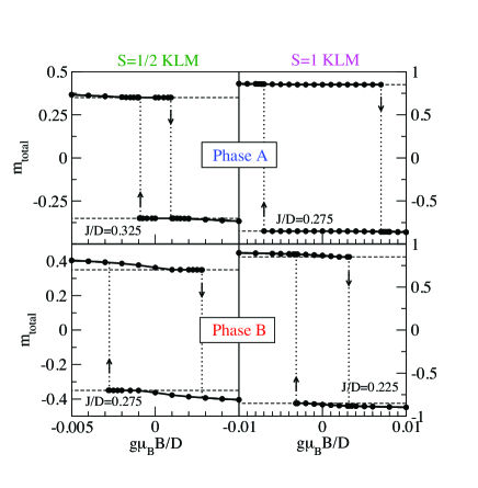
Figure 4: (Color online) Hysteresis loops: magnetization in longitudinal external magnetic field. The dashed lines indicate the value of the frozen magnetization $m_{S}$. The $g$-factors are assumed equal for $c$ and $f$ levels, $g_{c}=g_{f}=g$. Occupancy is $n=0.3$.

Does the existence of multiple phases indicate a competition between the exchange interaction and the Kondo effect? Some degree of antagonism is suggested by the fact that the $f$-shell magnetization $m_{f}$ has a minimum at the BA Lifshitz point where both tendencies are expected to be equally strong and, furthermore, it could be argued that $m_{f}$ increases with $J$ in phase A only because Kondo screening is rendered incomplete by the opening and widening of the gap. Nevertheless, this competition does not imply mutual exclusion and most results rather support the notion of robust coexistence.

Experimentally the phases can be distinguished by their magnetization curves. In phase A, $m_{\mathrm{total}}$ remains pinned to $m_{S}$ for a finite range of the field strength, while in phase B the susceptibility $dM/dB$ near zero field is finite, see Fig. 4. For sufficiently strong field, a gap opens in the minority band in phase B, too. This effect can be understood within a rigid-band picture. For very strong field, the magnetization is reoriented in a first-order spin-flop transition which preempts another Lifshitz transition.

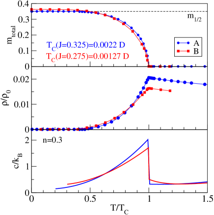
Figure 5: (Color online) Temperature dependence of the magnetization, resistivity and heat capacity for the spin-$1/2$ Kondo lattice model in phases A and B. The horizontal axis is rescaled by the Curie temperature $T_{C}$. Resistivity is in units of $\rho_{0}=2\pi e^{2}\Phi(0)/\hbar D$, where $\Phi$ is the transport integral. Heat capacity curve was obtained by differentiating a piecewise interpolation of the numerical results for the total energy.

In Fig. 5 we plot the temperature dependence of key thermodynamic and transport properties in phases A and B. We find that the magnetization in phase B remains essentially pinned at $m_{S}$ until $T$ becomes of the order of the gap, while it has a finite temperature-derivative at $T=0$ in phase A. This difference is, however, small. The resistance $\rho$ increases in both phases up to the Curie temperature $T_{c}$, then it decreases approximately as a power-law $T^{-0.3}$, not logarithmically. The heat capacity $c$ has a jump discontinuity at $T_{c}$. Similar features are indeed observed experimentally, for example in Refs. Tran et al. (2005); Colineau et al. (2008); Baumbach et al. (2012), although the simple KLM does not capture the full complexity of real materials.

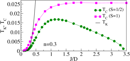
Figure 6: (Color online) “Ferromagnetic Doniach diagram” for spin-$1/2$ and spin-$1$ Kondo lattice models.

We summarize the behavior of both Kondo lattice models in the form of a “ferromagnetic Doniach diagram” in Fig. 6. We plot the Kondo temperature for a single-impurity model with flat band (which does not depend on the impurity spin Andrei et al. (1983)) and the Curie temperature $T_{C}$ for each model. The Curie temperature has no observable feature at the Lifshitz transition points $J^{*}$. Apart from the (approximately) factor of two difference, there is no difference in $T_{C}$ of spin-1/2 and spin-1 models for small $J$. At large $J$, spin-1/2 model first goes into the B’ phase and then becomes paramagnetic. The spin-1 model remains ferromagnetic in the large $J$ limit. This is similar to the behavior of the AFM phases of both models at half filling.

We conclude by answering the questions raised in the introduction. There is no Kondo breakdown and no criticality, but rather a continuous filling of the lower minority band and the disappearance of the electron pockets (and the emergence of hole pockets in the spin-1/2 model for large $J$). We find robust coexistence of FM order and Kondo screening in all phases, for both spins. Kondo underscreening does not need to be invoked to explain the magnetic ordering. Both models have qualitatively the same phase diagram for physically most relevant small $J$. The Lifshitz transitions are observable in the temperature and magnetic-field dependence of the magnetization. The static mean-field appears to be valid at the qualitative level, however to properly describe the real nature of ferromagnetic phases and transitions it is necessary to take into account dynamic effects, as in the DMFT treatment.

*

Supplemental Material

Appendix A Static mean-field theory

A.1 The $S=1/2$ case

We perform a mean-field decomposition in the KLM written in the form:

$$\mathcal{H}=\sum_{k,\sigma}\epsilon_{k}c_{k,\sigma}^{\dagger}c_{k,\sigma}+J\sum_{i}{\mathbf{s}}_{i}\cdot{\mathbf{S}}_{i}+\mu_{B}H\sum_{i}(g_{c}s_{z,i}+g_{f}S_{z,i}),$$ (3)

where $H$ is the external magnetic field oriented along the $z$ axis, $\mu_{B}$ the Bohr magneton, while $g_{c}$ and $g_{f}$ are the Landé factors. For simplicity, we consider flat non-interacting conduction-band density of states (DOS):

$$\rho_{c}^{0}=1/2D,$$ (4)

where $D$ is the half-bandwidth.

The interaction term for localized spins with $S=1/2$ is decomposed in terms of the hybridization operators Beach (2005); Viola Kusminskiy et al. (2008)

$$\chi^{\mu}=\frac{1}{\sqrt{2}}\sum_{\alpha,\beta}f^{\dagger}_{\alpha}\sigma^{\mu}_{\alpha\beta}c_{\beta},$$ (5)

where $c,f$ are annihilation operators for itinerant and localized electrons, respectively, and the spin indexes $\alpha$ and $\beta$ range over spin up and down. The index $\mu$ ranges over $0,1,2,3$; the operator $\sigma^{0}$ is the identity, while other $\sigma^{i}$ are the Pauli matrices. These operators are complete in the spin sector $1/2\otimes 1/2=1\oplus 0$, and therefore the interaction part can be split into:

$${\mathbf{s}}\cdot{\mathbf{S}}=\left(\frac{1}{2}c^{\dagger}\boldsymbol{\sigma}c\right)\cdot\left(\frac{1}{2}f^{\dagger}\boldsymbol{\sigma}f\right)=-3/4\chi^{0\dagger}\chi^{0}+1/4\boldsymbol{\chi}^{\dagger}\cdot\boldsymbol{\chi}.$$ (6)

This expression is exact.

We perform the standard mean-field procedure: $AB\approx\langle A\rangle B+A\langle B\rangle-\langle A\rangle\langle B\rangle$. We assume that only the singlet part $\langle\chi^{0}\rangle$ is nonzero and we use the $U(1)$ gauge freedom to make $\langle\chi_{0}\rangle$ real.

The second mean-field decomposition is done in the magnetic channel (assuming the magnetization is along the $z$ axis):

$${\mathbf{s}}\cdot{\mathbf{S}}=s_{z}\tilde{m}_{f}+\tilde{m}_{c}S_{z}-\tilde{m}_{c}\tilde{m}_{f},$$ (7)

where

$$\tilde{m}_{c}=\langle s^{z}\rangle\quad\text{and}\quad\tilde{m}_{f}=\langle S^{z}\rangle$$ (8)

are the expectation values of the $z$ component of conduction-band and localized-electron spin. These are proportional to the magnetization of $c(f)$ electrons:

$$m_{f(c)}=-\mu_{B}g_{f(c)}\tilde{m}_{f(c)}.$$ (9)

In order to fix the average number of electrons we introduce the chemical potential $\mu$. We also introduce Lagrangian multipliers $\lambda_{i}$ to enforce the local constraint $\langle n_{f,i}\rangle=1$ on the $f$ electrons:

$$\sum_{i}\lambda_{i}\sum_{\sigma}\left(f^{\dagger}_{i,\sigma}f_{i,\sigma}-1\right).$$ (10)

This constraint is fulfilled only as an average over all $f$ electrons, $\lambda_{i}\equiv\lambda$. We may then perform a FT:

$$\lambda\sum_{k}\sum_{\sigma}\left(f^{\dagger}_{k\sigma}f_{k\sigma}-1\right).$$ (11)

Thus $\lambda$ plays the role of the effective $f$ level energy: the $f$ level occupancy is controlled by the difference between $\lambda$ and $\mu$.

At constant $\mu$, the thermodynamic potential that we need to minimize is

$$K(\mu,\ldots)=H(N_{\mathrm{total}},\ldots)-\mu N_{\mathrm{total}}=H-\mu(N_{c}+N_{f})=H-\mu\sum_{k,\sigma}\left(c^{\dagger}_{k\sigma}c_{k\sigma}+f^{\dagger}_{k\sigma}f_{k\sigma}\right).$$ (12)

The mean-field thermodynamic potential takes the following wave-vector representation:

$$\mathcal{K}_{MF}=\sum_{k\sigma}\left(c^{\dagger}_{k,\sigma}\,f^{\dagger}_{k,\sigma}\right)\tilde{M}_{k}\begin{pmatrix}c_{k,\sigma}\\ f_{k,\sigma}\end{pmatrix}+\sum_{k}E_{0},$$ (13)

where the matrix $M_{k}$ is

$$\tilde{M}_{k}=\begin{pmatrix}\epsilon_{k,\sigma}-\mu&-c\chi_{0}\\ -c\chi_{0}&\lambda_{\sigma}-\mu\end{pmatrix}.$$ (14)

with

$$\epsilon_{k,\sigma}=\epsilon_{k}+\epsilon_{\sigma}=\epsilon_{k}+J\tilde{m}_{f}\frac{\sigma}{2}+\mu_{B}g_{c}H\frac{\sigma}{2}=\epsilon_{k}+\mu_{B}g_{c}\tilde{H}_{c}\frac{\sigma}{2},$$ (15)

$$\lambda_{\sigma}=\lambda+J\tilde{m}_{c}\frac{\sigma}{2}+\mu_{B}g_{f}H\frac{\sigma}{2}=\lambda+\mu_{B}g_{f}\tilde{H}_{f}\frac{\sigma}{2},$$ (16)

$$c=\frac{3}{4}\frac{1}{\sqrt{2}}J=\frac{3J}{4\sqrt{2}},$$ (17)

$$E_{0}=+\frac{3}{4}J\chi_{0}^{2}-J\tilde{m}_{c}\tilde{m}_{f}-\lambda.$$ (18)

The effective field felt by the $c(f)$ electrons is given by

$$\tilde{H}_{c(f)}=H+\frac{J\tilde{m}_{f(c)}}{\mu_{B}g_{c(f)}}.$$ (19)

In general, the equation of motion (EOM) can be written as

$$z\langle\langle A,B\rangle\rangle=-\langle\langle[\mathcal{K}_{MF},A],B\rangle\rangle+\langle\langle[A,B]\rangle\rangle,$$ (20)

where $A,B$ are arbitrary fermionic operators. We find

$$\begin{split}zG_{cc,k\sigma}&=1+\left(\epsilon_{k\sigma}-\mu\right)G_{cc,k\sigma}-c\chi_{0}G_{fc,k\sigma},\\ zG_{ff,k\sigma}&=1+\left(\lambda_{\sigma}-\mu\right)G_{ff,k\sigma}-c\chi_{0}G_{cf,k\sigma},\\ zG_{cf,k\sigma}&=(\epsilon_{k\sigma}-\mu)G_{cf,k\sigma}-c\chi_{0}G_{ff,k\sigma},\\ zG_{fc,k\sigma}&=(\lambda_{\sigma}-\mu)G_{fc,k\sigma}-c\chi_{0}G_{cc,k\sigma}.\end{split}$$ (21)

Note also that $G_{cf}(z)=G_{fc}(z)$, since the matrix $\tilde{M}_{k}$ is symmetric. It follows

$$\begin{split}(z-\epsilon_{k\sigma}+\mu)G_{cc,k\sigma}&=1-c\chi_{0}G_{fc,k\sigma},\\ (z-\lambda_{\sigma}+\mu)G_{ff,k\sigma}&=1-c\chi_{0}G_{cf,k\sigma},\\ (z-\epsilon_{k\sigma}+\mu)G_{cf,k\sigma}&=-c\chi_{0}G_{ff,k\sigma},\\ (z-\lambda_{\sigma}+\mu)G_{fc,k\sigma}&=-c\chi_{0}G_{cc,k\sigma},\end{split}$$ (22)

and consequently

$$(z-\lambda_{\sigma}+\mu)^{2}G_{ff,k\sigma}=(c\chi_{0})^{2}G_{cc,k\sigma}.$$ (23)

In this approach, writing $z=\omega+i\delta$, the Fermi level corresponds to $\omega=0$. We use a different convention. We absorb $\mu$ into $z$: $\tilde{z}=z+\mu$. Also the Green’s functions take $\tilde{z}$ as their argument. With this choice, spectral functions are obtained with replacement $\tilde{z}=\omega+i\delta$ and there are no explicit $\mu$ in the expressions for Green’s functions. $\mu$ only appears as an integration limit (or in the Fermi-Dirac distribution). We drop writing the tilde in $\tilde{z}$ in the following.

The quasiparticle band edges are

$$\begin{split}\omega_{1,\sigma}&=\frac{1}{2}\left(\epsilon_{\sigma}+\lambda_{\sigma}-D-\sqrt{(\epsilon_{\sigma}-\lambda_{\sigma}-D)^{2}+4c^{2}\chi_{0}^{2}}\right),\\ \omega_{2,\sigma}&=\frac{1}{2}\left(\epsilon_{\sigma}+\lambda_{\sigma}+D-\sqrt{(\epsilon_{\sigma}-\lambda_{\sigma}+D)^{2}+4c^{2}\chi_{0}^{2}}\right),\\ \omega_{3,\sigma}&=\frac{1}{2}\left(\epsilon_{\sigma}+\lambda_{\sigma}-D+\sqrt{(\epsilon_{\sigma}-\lambda_{\sigma}-D)^{2}+4c^{2}\chi_{0}^{2}}\right),\\ \omega_{4,\sigma}&=\frac{1}{2}\left(\epsilon_{\sigma}+\lambda_{\sigma}+D+\sqrt{(\epsilon_{\sigma}-\lambda_{\sigma}+D)^{2}+4c^{2}\chi_{0}^{2}}\right).\end{split}$$ (24)

In the multiindex $(i,\sigma)$, $\sigma$ is spin, while $i$ enumerates the band edges from the lowest to the highest. Furthermore

$$\epsilon_{\sigma}=J\tilde{m}_{f}\frac{\sigma}{2}+\mu_{B}g_{c}H\frac{\sigma}{2}=\mu_{B}g_{c}\tilde{H}_{c}\frac{\sigma}{2}.$$ (25)

The final closed-form expressions for the spectral functions are

$$\rho_{c,\sigma}(\omega)=\rho_{c}^{0}\sum_{i=1}^{4}(-1)^{i-1}\theta(\omega-\omega_{i,\sigma}),$$ (26)

$$\rho_{f,\sigma}(\omega)=\frac{(c\chi_{0})^{2}}{(\omega-\lambda_{\sigma})^{2}}\rho_{c,\sigma}(\omega).$$ (27)

We also have

$$\rho_{cf,\sigma}(\omega)=-\frac{c\chi_{0}}{\omega-\lambda_{\sigma}}\rho_{c,\sigma}(\omega).$$ (28)

The energy eigenvalues are

$$E_{k,\sigma}=\frac{1}{2}\left(\epsilon_{k,\sigma}+\lambda_{\sigma}\pm\sqrt{(\epsilon_{k,\sigma}-\lambda_{\sigma})^{2}+4c^{2}\chi_{0}^{2}}\right).$$ (29)

A.1.1 Mean-field equations

We can derive the system of mean-field equation using the fluctuation-dissipation theorem at $T=0$:

$$\begin{split}\langle AB\rangle&=-\int_{\mu}^{\infty}\frac{d\omega}{\pi}G^{\prime\prime}_{AB}(\omega)\\ &=\int_{-\infty}^{\mu}d\omega\rho_{BA}(\omega).\end{split}$$ (30)

We obtain

$$n_{c}=\sum_{\sigma}\langle c^{\dagger}_{\sigma}c_{\sigma}\rangle=\sum_{\sigma}\int d\omega\rho_{c,\sigma}(\omega),$$ (31)

$$1=n_{f}=\sum_{\sigma}\langle f^{\dagger}_{\sigma}f_{\sigma}\rangle=\sum_{\sigma}\int d\omega\rho_{f,\sigma}(\omega),$$ (32)

$$\tilde{m}_{c}=1/2\sum_{\sigma}\sigma\langle c^{\dagger}_{\sigma}c_{\sigma}\rangle=1/2\sum_{\sigma}\int\sigma d\omega\rho_{c,\sigma}(\omega),$$ (33)

$$\tilde{m}_{f}=1/2\sum_{\sigma}\sigma\langle f^{\dagger}_{\sigma}f_{\sigma}\rangle=1/2\sum_{\sigma}\int\sigma d\omega\rho_{f,\sigma}(\omega).$$ (34)

In all integrals, the lower integration limit is $-\infty$, while the upper is the chemical potential $\mu$.

For the gap equation we take the symmetrized spectral function

$$A_{cf,\sigma}=-\frac{1}{2\pi}[\mathrm{Im}G_{cf}(\omega+i\delta)+\mathrm{Im}G_{fc}(\omega+i\delta)]=\rho_{cf,\sigma}.$$

This gives:

$$\frac{1}{2}\langle f_{\uparrow}^{\dagger}c_{\uparrow}+c_{\uparrow}^{\dagger}f_{\uparrow}+f_{\downarrow}^{\dagger}c_{\downarrow}+c_{\downarrow}^{\dagger}f_{\downarrow}\rangle=\frac{1}{2}2\sqrt{2}\langle\chi_{0}\rangle=$$ (35)

$$\sum_{\sigma}\int d\omega A_{fc,\sigma}(\omega)=-c\chi_{0}\sum\int d\omega\frac{1}{\omega-\lambda_{\sigma}}\rho_{c,\sigma}(\omega)$$ (36)

We now assume $\chi_{0}\neq 0$. Using $c=3J/(4\sqrt{2})$, we finally find the gap equation

$$\boxed{\sum_{\sigma}\int_{-\infty}^{\mu}d\omega\frac{\rho_{c,\sigma}(\omega)}{\omega-\lambda_{\sigma}}=-8/3J.}$$ (37)

This set of non-linear equations had been previously derived in Refs. Beach (2005); Viola Kusminskiy et al. (2008), while in Ref. Li and Zhang (2010) a somewhat different mean-field decoupling was used.

A.1.2 Evaluation of energy

The total energy can be evaluated as

$$\begin{split}E_{\mathrm{GS}}&=\left\langle H_{\mathrm{MF}}\right\rangle\\ &=\sum_{k}\left\langle\sum_{ij}c_{ki}^{\dagger}c_{kj}M_{k,ij}+E_{0}\right\rangle\\ &=\sum_{k}\left(\sum_{ij}\int_{-\infty}^{\mu}A_{\epsilon_{k},ij}(\omega)M_{\epsilon_{k},ij}\mathrm{d}\omega+E_{0}\right).\end{split}$$ (38)

We used a symmetrized spectral function

$$A_{ij}(\omega)=\frac{1}{2}\left[-\frac{1}{\pi}\mathrm{Im}G_{ij}(\omega+i\delta)-\frac{1}{\pi}\mathrm{Im}G_{ji}(\omega+i\delta)\right],$$ (39)

since

$$\int_{-\infty}^{\mu}A_{ij}(\omega)\mathrm{d}\omega=\frac{1}{2}\langle c^{\dagger}_{i}c_{j}+c^{\dagger}_{j}c_{i}\rangle.$$ (40)

Then

$$\begin{split}\frac{E_{\mathrm{GS}}}{N}&=E_{0}+\int_{-D}^{D}\rho(\epsilon)d\epsilon\int_{-\infty}^{\mu}\mathrm{Tr}[\mathbf{A}_{\epsilon}(\omega)\mathbf{M}_{\epsilon}]\mathrm{d}\omega.\end{split}$$ (41)

Note that both $\mathbf{A}$ and $\mathbf{M}$ have out-of-diagonal matrix elements. Now we use

$$\mathrm{Tr}[\mathbf{A}(\omega)\mathbf{M}]=-\frac{1}{\pi}\mathrm{Im}\mathrm{Tr}[\mathbf{G}(\omega+i\delta)\mathbf{M}]=-\frac{1}{\pi}\mathrm{Im}\mathrm{Tr}[(\omega+i\delta-\mathbf{M})^{-1}\mathbf{M}]=-\frac{1}{\pi}\mathrm{Im}\mathrm{Tr}[(\omega+i\delta-\mathbf{M})^{-1}\omega]=\mathrm{Tr}[\mathbf{A}(\omega)]\omega,$$ (42)

which follows from the fact that $\mathrm{Im}[1/(z-x)]$ is a delta distribution, and we have used a transformation to the eigenbasis and back to replace $\mathbf{M}$ by $\omega$ in the third step. Thus, after the integration over $\epsilon$,

$$\frac{E_{\mathrm{GS}}}{N}=E_{0}+\sum_{\sigma}\int_{-\infty}^{\mu}\omega d\omega\left[\rho_{c,\sigma}(\omega)+\rho_{f,\sigma}(\omega)\right].$$ (43)

We also have

$$\begin{split}\frac{N_{c}+N_{f}}{N}&=\int_{-D}^{D}\rho(\epsilon)d\epsilon\int_{-\infty}^{\mu}\mathrm{Tr}[A_{\epsilon}(\omega)]d\omega\\ &=\sum_{\sigma}\int_{-\infty}^{\mu}\left[\rho_{c,\sigma}(\omega)+\rho_{f,\sigma}(\omega)\right]d\omega,\end{split}$$ (44)

thus finally,

$$\frac{K_{\mathrm{GS}}}{N}=E_{0}+\sum_{\sigma}\int_{-\infty}^{\mu}d\omega(\omega-\mu)\left[\rho_{c,\sigma}(\omega)+\rho_{f,\sigma}(\omega)\right].$$ (45)

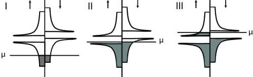
Figure 7: Sketch of the possible placements of the bands with respect to the chemical potential. The phase I correspond to the phase B’, phase II to the phase A and phase III to the phase B in the DMFT calculations.

We would like to evaluate Eq. (45) for two different cases represented on Fig. 7, namely cases I and II:

$$\begin{split}\frac{K_{GS}}{N}&=E_{0}+\sum\limits_{\sigma}\int_{-\infty}^{\mu}d\omega(\omega-\mu)\left(1+\frac{(c\chi_{0})^{2}}{(\omega-\lambda_{\sigma})^{2}}\right)\rho_{c\sigma}(\omega)\\ &=E_{0}+E_{c}+(c\chi_{0})^{2}\sum_{\sigma}\int_{-\infty}^{\mu}d\omega\frac{\omega-\lambda_{\sigma}+\lambda_{\sigma}-\mu}{(\omega-\lambda_{\sigma})^{2}}\rho_{c\sigma}(\omega)\\ &=E_{0}+E_{c}+(c\chi_{0})^{2}\sum\limits_{\sigma}\int_{-\infty}^{\mu}d\omega\frac{\rho_{c,\sigma}(\omega)}{\omega-\lambda_{\sigma}}+\sum\limits_{\sigma}(\lambda_{\sigma}-\mu)n_{f,\sigma}\\ &=E_{0}+E_{c}+(c\chi_{0})^{2}(-8/3J)+\sum\limits_{\sigma}(\lambda_{\sigma}-\mu)n_{f,\sigma},\end{split}$$ (46)

where $E_{c}=\int_{-\infty}^{\mu}d\omega(\omega-\mu)\rho_{c,\sigma}(\omega)$ and in the last line we have use the gap equation, see Eq. (37). We need to evaluate

$$\begin{split}2\sum_{\sigma}(\lambda_{\sigma}-\mu)n_{f,\sigma}&=\sum_{\sigma}\left(\lambda-\mu+\mu_{B}g_{f}\tilde{H}_{f}\frac{\sigma}{2}\right)n_{f\sigma}\\ &=(\lambda-\mu)n_{f}+2\mu_{B}g_{f}\tilde{H}_{f}\tilde{m}_{f}.\end{split}$$ (47)

For $H=0$, this is equal to

$$(\lambda-\mu)n_{f}+J\tilde{m}_{c}\tilde{m}_{f}.$$ (48)

Case I is when $\omega_{1,\sigma}<\mu<\omega_{2,\sigma}$ for both spin orientations. We can write:

$$E_{c}=\rho_{c,0}\sum\limits_{\sigma}[(\mu^{2}-\omega_{1,\sigma}^{2})/2]-\mu n_{c}$$ (49)

and

$$\begin{split}\frac{K_{GS}}{N}&=\frac{3}{4}J\chi_{0}^{2}-J\tilde{m}_{c}\tilde{m}_{f}-\lambda+\rho_{c,0}\sum\limits_{\sigma}[(\mu^{2}-\omega_{1,\sigma}^{2})/2]-\mu n_{c}-\frac{3}{4}J\chi_{0}^{2}+\sum\limits_{\sigma}(\lambda_{\sigma}-\mu)n_{f,\sigma}\\ &=-J\tilde{m}_{c}m_{f}-\lambda+\rho_{c,0}\sum\limits_{\sigma}[(\mu^{2}-\omega_{1,\sigma}^{2})/2]-\mu n_{c}+(\lambda-\mu)n_{f}+J\tilde{m}_{c}\tilde{m}_{f}\\ &=\rho_{c,0}\sum\limits_{\sigma}[(\mu^{2}-\omega_{1,\sigma}^{2})/2]-\mu[n_{c}+n_{f}]\end{split}$$ (50)

where in the second line we have used Eq. (48) and in the last line $\langle n_{f}\rangle=1.$

Case II is when $\omega_{2,\uparrow}<\mu<\omega_{3,\uparrow}$ and only difference is that $\mu\rightarrow\omega_{2,\uparrow}$ in integration limit for $\uparrow$ c electrons. Therefore, the only difference is in the evaluation of $E_{c}$:

$$E_{c}=\rho_{c}^{0}\left(\frac{\mu^{2}-\omega_{1,\downarrow}^{2}}{2}+\frac{\omega_{2,\uparrow}^{2}-\omega_{1,\uparrow}^{2}}{2}\right)-\mu n_{c}.$$ (51)

A.2 The $S=1$ case

We next proceed with an analogous treatment for the $S=1$ problem. We decompose the interaction term into doublet and quadruplet terms, $1/2\otimes 1=1/2\oplus 3/2$. We find:

$${\mathbf{s}}\cdot{\mathbf{S}}=-\sum\limits_{i=1}^{2}\chi_{d,i}^{\dagger}\chi_{d,i}+(1/2)\sum\limits_{i=1}^{4}\chi_{q,i}^{\dagger}\chi_{q,i},$$ (52)

where $\chi_{d,i}(\chi_{q,j})$ are the doublet ($i=1,2$) and the quadruplet ($j=1,2,3,4$) sets of operators under the spin $SU(2)$ symmetry, namely:

$$\chi_{d,1}=-\sqrt{1/3}c_{\downarrow}^{\dagger}f_{0}-\sqrt{2/3}c_{\uparrow}^{\dagger}f_{1},\qquad\chi_{d,2}=\sqrt{2/3}c_{\downarrow}^{\dagger}f_{-1}+\sqrt{1/3}c_{\uparrow}^{\dagger}f_{0},$$ (53)

$$\chi_{q,1}=-c_{\uparrow}^{\dagger}f_{-1},\quad\chi_{q,2}=-\sqrt{1/3}c_{\downarrow}^{\dagger}f_{-1}+\sqrt{2/3}c_{\uparrow}^{\dagger}f_{0},\quad\chi_{q,3}=\sqrt{2/3}c_{\downarrow}^{\dagger}f_{0}-\sqrt{1/3}c_{\uparrow}^{\dagger}f_{1},\quad\chi_{q,4}=-c_{\downarrow}^{\dagger}f_{1}.$$ (54)

These operators again form a complete set in the spin sector. The decomposition in Eq. (52) is exact.

We focus on the doublet part and set all quadruplet fields to zero, $\langle\chi_{q,j}\rangle=0.$ We explicitly break the SU(2) symmetry by setting $\langle\chi_{d,2}\rangle=0$ and use the $U(1)$ gauge freedom to make $\langle\chi_{d,1}\rangle$ real. In analogy with the $S=1/2$ case, we make a second mean-field decomposition in the magnetic channel. The mean-field Hamiltonian has a simple wave-vector representation:

$$\mathcal{K}_{MF}=\sum\limits_{k}\left(c_{k,\downarrow}^{\dagger}\,c_{k,\uparrow}^{\dagger}\,f_{k,-1}^{\dagger}\,f_{k,0}^{\dagger}\,f_{k,+1}^{\dagger}\right)\tilde{M}_{k}\begin{pmatrix}c_{k,\downarrow}\\ c_{k,\uparrow}\\ f_{k,-1}\\ f_{k,0}\\ f_{k,+1}\end{pmatrix}+\sum_{k}E_{0},$$ (55)

where the matrix $\tilde{M}_{k}$ is

$$\begin{pmatrix}\epsilon_{k,\downarrow}-\mu&0&0&J\chi_{d,1}/\sqrt{3}&0\\ 0&\epsilon_{k,\uparrow}-\mu&0&0&\sqrt{2/3}J\chi_{d,1}\\ 0&0&\lambda_{-1}-\mu&0&0\\ J\chi_{d,1}/\sqrt{3}&0&0&\lambda_{0}-\mu&0\\ 0&\sqrt{2/3}J\chi_{d,1}&0&0&\lambda_{1}-\mu\end{pmatrix}$$ (56)

and

$$\epsilon_{k,\sigma}=\epsilon_{k}+J\tilde{m}_{f}\frac{\sigma}{2}+\mu_{B}g_{c}H\frac{\sigma}{2}=\epsilon_{k}+\mu_{B}g_{c}\tilde{H}_{c}\frac{\sigma}{2},$$ (57)

$$\lambda_{i}=\lambda+J\tilde{m}_{c}i+\mu_{B}g_{f}Hi=\lambda+\mu_{B}g_{f}\tilde{H}_{f}i,$$ (58)

$$E_{0}=J\chi_{d,1}^{2}-J\tilde{m}_{c}\tilde{m}_{f}-\lambda,$$ (59)

with $\sigma=\pm 1$, $i=-1,0,1$. The effective field felt by the $c(f)$ electrons is given by

$$\tilde{H}_{c(f)}=H+\frac{J\tilde{m}_{f(c)}}{\mu_{B}g_{c(f)}}.$$ (60)

The EOMs are

$$\begin{split}(z-\epsilon_{k,\downarrow}+\mu)&G_{c_{\downarrow},k}=1+\sqrt{\frac{1}{3}}J\chi_{d1}G_{f_{0},c_{\downarrow},k}\\ (z-\epsilon_{k,\uparrow}+\mu)&G_{c_{\uparrow},k}=1+\sqrt{\frac{2}{3}}J\chi_{d1}G_{f_{1},c_{\uparrow},k}\\ (z-\lambda_{-1}+\mu)&G_{f_{-1},k}=1\\ (z-\lambda_{0}+\mu)&G_{f_{0},c_{\downarrow},k}=\sqrt{\frac{1}{3}}J\chi_{d1}G_{c_{\downarrow},c_{\downarrow},k}\\ (z-\epsilon_{k,\downarrow}+\mu)&G_{c_{\downarrow}f_{0},k}=\sqrt{\frac{1}{3}}J\chi_{d1}G_{f_{0},f_{0},k}\\ \end{split}$$ (61)

and note also that $G_{ij,k}(z)=G_{ji,k}(z),$ while for the diagonal elements we used $G_{ii,k}(z)=G_{i,k}(z).$ Consequently

$$\begin{split}(z-\lambda_{0}+\mu)^{2}G_{f_{0},k}&=(z-\lambda_{0}+\mu)\left(1+\frac{(J\chi_{d1})^{2}}{3}G_{c_{\downarrow},k}\right)\\ (z-\lambda_{1}+\mu)^{2}G_{f_{1},k}&=(z-\lambda_{1}+\mu)\left(1+\frac{2(J\chi_{d1})^{2}}{3}G_{c_{\uparrow},k}\right).\end{split}$$ (62)

Once more we absorb $\mu$ into $z$: $\tilde{z}=z+\mu$ and drop writing tilde in $\tilde{z}$ in the following. The quasiparticles band edges $\omega_{i,\sigma}$ are:

$$\omega_{1,\sigma}=\left(3\epsilon_{\sigma}-3D+3\lambda_{\sigma}-\sqrt{9(\epsilon_{\sigma}-D-\lambda_{\sigma})^{2}+12F_{\sigma}(J\chi_{d,1})^{2}}\right)/6$$

$$\omega_{2,\sigma}=\left(3\epsilon_{\sigma}+3D+3\lambda_{\sigma}-\sqrt{9(\epsilon_{\sigma}+D-\lambda_{\sigma})^{2}+12F_{\sigma}(J\chi_{d,1})^{2}}\right)/6$$

$$\omega_{3,\sigma}=\left(3\epsilon_{\sigma}-3D+3\lambda_{\sigma}+\sqrt{9(\epsilon_{\sigma}-D-\lambda_{\sigma})^{2}+12F_{\sigma}(J\chi_{d,1})^{2}}\right)/6$$

$$\omega_{4,\sigma}=\left(3\epsilon_{\sigma}+3D+3\lambda_{\sigma}+\sqrt{9(\epsilon_{\sigma}+D-\lambda_{\sigma})^{2}+12F_{\sigma}(J\chi_{d,1})^{2}}\right)/6,$$ (63)

where $\epsilon_{\sigma}$ has been defined in the section on the $S=1/2$ model, while

$$F(1)=2,\quad F(-1)=1.$$ (64)

and, furthermore,

$$\lambda_{\downarrow}=\lambda_{0},$$ (65)

$$\lambda_{\uparrow}=\lambda_{1}.$$ (66)

The spectral functions are given by:

$$\rho_{c,\sigma}(\omega)=\rho_{c}^{0}\sum\limits_{i=1}^{4}(-1)^{i-1}\theta(\omega-\omega_{i,\sigma}),$$ (67)

$$\rho_{f,-1}(\omega)=\delta(\omega-\lambda_{-1}),$$ (68)

$$\rho_{f,0}(\omega)=F_{-1}\frac{(J\chi_{d,1})^{2}}{3(z-\lambda_{0})^{2}}\rho_{c,\downarrow}(\omega),$$ (69)

$$\rho_{f,1}(\omega)=F_{1}\frac{(J\chi_{d,1})^{2}}{3(z-\lambda_{1})^{2}}\rho_{c,\uparrow}(\omega).$$ (70)

$$\rho_{f_{1}c_{\uparrow}}(\omega)=\sqrt{\frac{2}{3}}\frac{(J\chi_{d,1})}{(\omega-\lambda_{1})}\rho_{c_{\uparrow}}(\omega).$$ (71)

$$\rho_{f_{0}c_{\downarrow}}(\omega)=\sqrt{\frac{1}{3}}\frac{(J\chi_{d,1})}{(\omega-\lambda_{0})}\rho_{c_{\downarrow}}(\omega).$$ (72)

The $f_{-1}$ must be unoccupied, otherwise the number of $f$ electrons cannot be exactly 1. Thus $\lambda_{-1}>\mu$. This also implies that $f_{-1}$ must be the highest in energy of the $f$ states, thus $\tilde{m}_{c}<0$ and consequently $\tilde{m}_{f}>0$.

A.2.1 The mean-field equations

Using the fluctuaction-dissipation theorem at $T=0$, we find

$$n_{c}=\sum_{\sigma}\langle c^{\dagger}_{\sigma}c_{\sigma}\rangle=\sum_{\sigma}\int d\omega\rho_{c,\sigma}(\omega),$$ (73)

$$1=n_{f}=\sum_{i}\langle f^{\dagger}_{i}f_{i}\rangle=\sum_{i}\int d\omega\rho_{f,i}(\omega),$$ (74)

$$\tilde{m}_{c}=1/2\sum_{\sigma}\sigma\langle c^{\dagger}_{\sigma}c_{\sigma}\rangle=1/2\sum_{\sigma}\int\sigma d\omega\rho_{c,\sigma}(\omega),$$ (75)

$$\tilde{m}_{f}=\sum_{i}i\langle f^{\dagger}_{i}f_{i}\rangle=\sum_{i}i\int d\omega\rho_{f,i}(\omega).$$ (76)

For the gap equation we take symmetrized spectral function $A_{c\sigma;fi}=-\frac{1}{2\pi}[\mathrm{Im}G_{c\sigma;fi}(\omega+i\delta)+\mathrm{Im}G_{fi;c\sigma}(\omega+i\delta)]=\rho_{c\sigma;f,i},$ where $G_{c\sigma;fi}(z)=\langle\langle c^{\dagger}_{\sigma};f_{i}\rangle\rangle_{z}$, etc. For the evaluation of $\langle\chi_{1}\rangle$ we will need two off-diagonal spectral functions:

$$\rho_{c\downarrow;f0}=\frac{J\chi_{1}}{\sqrt{3}(z-\lambda_{0})}\rho_{c\downarrow}(\omega)$$ (77)

$$\rho_{c\uparrow;f1}=\frac{\sqrt{2/3}J\chi_{1}}{z-\lambda_{1}}\rho_{c\uparrow}(\omega).$$ (78)

The expectation value is

$$\langle\chi_{1}\rangle=\frac{1}{2}[-\sqrt{1/3}(\langle c_{\downarrow}^{\dagger}f_{0}+f_{0}^{\dagger}c_{\downarrow}\rangle)-\sqrt{2/3}(c_{\uparrow}^{\dagger}f_{1}+f_{1}^{\dagger}c_{\uparrow})]=-\sqrt{1/3}\int A_{c\downarrow,f0}(\omega)d\omega-\sqrt{2/3}\int A_{c\uparrow,f1}(\omega)d\omega$$ (79)

$$=-\sqrt{1/3}\frac{J\chi_{1}}{\sqrt{3}}\int d\omega\rho_{c\downarrow}/(\omega-\lambda_{0})-\sqrt{2/3}\sqrt{2/3}J\chi_{1}\int d\omega\rho_{c,\uparrow}(\omega)/(\omega-\lambda_{1})$$ (80)

$$=-(J\chi_{1}/3)\left[\int d\omega\rho_{c,\downarrow}(\omega)/(\omega-\lambda_{0})\right]-2J\chi_{1}/3\left[\int d\omega\rho_{c\uparrow}(\omega)/(\omega-\lambda_{1})\right].$$ (81)

Finally, we obtain the gap equation:

$$\boxed{\int d\omega\rho_{c\downarrow}(\omega)/(\omega-\lambda_{0})+2\int d\omega\rho_{c\uparrow}(\omega)/(\omega-\lambda_{1})=-3/J.}$$ (82)

This equation has essentially the same structure as the gap equation for the $S=1/2$ case.

A.2.2 Evaluation of energy

The total energy can be evaluated in analogy to the $S=1/2$ case. We find

$$\frac{{K_{\mathrm{GS}}}}{N}=E_{0}+\sum\limits_{\sigma}\int_{-\infty}^{\mu}d\omega(\omega-\mu)[\rho_{c,\sigma}(\omega)+\rho_{f,i(\sigma)}(\omega)]+(\lambda_{-1}-\mu)\theta(\omega-\lambda_{-1})$$ (83)

We evaluate Eq. 83 for two different cases represented on Fig. 7. For case I, $E_{c}=\rho_{c,0}\sum\limits_{\sigma}[(\mu^{2}-\omega_{1,\sigma}^{2})/2]-\mu n_{c}$, thus

$$\begin{split}\frac{K_{GS}}{N}&=\rho_{c,0}\sum\limits_{\sigma}[(\mu^{2}-\omega_{1,\sigma}^{2})/2]+\lambda(n_{f0}+n_{f1})-\mu(n_{f}+n_{c})\end{split}$$ (84)

In the case II,

$$E_{c}=\rho_{c}^{0}\left(\frac{\mu^{2}-\omega_{1,\downarrow}^{2}}{2}+\frac{\omega_{2,\uparrow}^{2}-\omega_{1,\uparrow}^{2}}{2}\right)-\mu n_{c}.$$ (85)

Appendix B Phase diagrams for $S=1/2$ and $S=1$

We now discuss the different possible mean-field phases for the $S=1/2$ and $S=1$ Kondo lattice models.

One possible phase is a pure saturated ferromagnetic phase with magnetization $m_{f}=-g_{f}\mu_{B}S$ and with zero hybridisation, $\chi_{d,1}=0$. If conducting electrons are completely polarized we call it the polar phase and the magnetization of conducting electrons is then given by

$$m_{c,P-I}=\mu_{B}g_{c}n_{c}/2.$$ (86)

For intermediate coupling regime, we distinguish between the ferromagnetic phases I, II, and III, which all have a finite value of the hybridisation parameter $\chi_{d,1}$ (thus a spectral gap). They are schematically represented in in Fig. 7. The phase I with the electron pockets, corresponds to the phase B’ in the DMFT calculations. The phase II with the chemical potential in the gap corresponds to the DMFT phase A. The numerical results in the phase II clearly indicate that as we lower $J$ the transition into phase III is expected, but when $\mu>\omega_{3,\uparrow}$ we were not able to find convergent solution in the regime of small $J$, as marked by the the dashed line in Fig. 8, see also Viola Kusminskiy et al. (2008). This phase III would correspond to the phase B in the DMFT calculations, where this is a stable phase.

The phase boundary between the phase I and II or between the phase II and III is given by the condition

$$\tilde{m}_{c}+\tilde{m}_{f}=(2S-n)/2,$$ (87)

for the expectation values of spin $z$ component, which shows plateau behaviour irrespective of the Landé factors or, equivalently,

$$m_{c}/g_{c}+m_{f}/g_{f}=-\mu_{B}(2S-n)/2.$$ (88)

This is equivalent to the condition that

$$\mu=\omega_{2(3),\uparrow}$$ (89)

for transition between the phases I$\rightarrow$ II (II$\rightarrow$ III).

The pure Kondo singlet (paramagnetic) phase is defined by $m_{c}=0,m_{f}=0,\chi_{d,1}\neq 0$. We only find it for $S=1/2$. In the $S=1$ model the hole pocket never emerges; instead, the chemical potential becomes attached near the top of the bottom band for large $J$. In fact, similar behavior is also observed in the DMFT solutions. The boundary between phase I and the Kondo phase is determined by the condition

$$m_{f}=m_{c}=0.$$ (90)

The boundary between the phases I,II and polar-I is given by the condition

$$\chi_{d,1}=0.$$ (91)

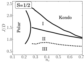
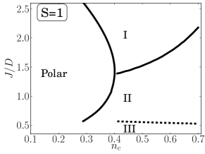
Figure 8: Ground state phase diagram of the KLM: (a) $S=1/2$, (b) $S=1$ with Landé factors $g_{c}=g_{f}=1.$ For the description of phases I, II, see the discussion in the text and Fig. 7. Phase Polar-I represent polarized phase with zero hybridisation and Kondo phase is paramagnetic phase ($m_{c}=m_{f}=0.$). The dashed line represent the transition into phase where we could not find the convergent solution, but phase III is expected, see discussion in the text.

We conclude that the qualitative features of the static MF and DMFT phase diagrams are rather similar, except that in the static mean-field theory the phase III is not stable. The main difference compared to previous works Beach et al. (2004); Viola Kusminskiy et al. (2008); Li and Zhang (2010) is the finding that in the MF treatment the metamagnetic transition is described by the transition I $\rightarrow$ II, while in the DMFT there are two different scenarios for metamagnetic transitions, either the transition I $\rightarrow$ II or the transition II $\rightarrow$ III, where only the former is expected for physically relevant model parameters.

References

Coleman and Schofield (2005)
P. Coleman and
A. J. Schofield,
Nature 433,
226 (2005).
Löhneysen et al. (2007)
H. Löhneysen,
A. Rosch,
M. Vojta, and
P. Wölfle,
Reviews of Modern Physics 79,
1015 (2007).
Si and Steglich (2010)
Q. Si and
F. Steglich,
Science 329,
1161 (2010).
Stewart (2001)
G. R. Stewart,
Reviews of Modern Physics 73,
797 (2001).
Gegenwart et al. (2008)
P. Gegenwart,
Q. Si, and
F. Steglich,
Nature Physics 4,
186 (2008).
Pfleiderer (2009)
C. Pfleiderer,
Reviews of Modern Physics 81,
1551 (2009).
Tsunetsugu et al. (1997)
H. Tsunetsugu,
M. Sigrist, and
K. Ueda,
Reviews of Modern Physics 69,
809 (1997).
Gulácsi (2004)
M. Gulácsi,
Advances in Physics 53,
769 (2004).
Hewson (1993)
A. C. Hewson,
The Kondo Problem to Heavy-Fermions
(Cambridge University Press, Cambridge,
1993).
Doniach (1977)
S. Doniach,
Physica B 91,
231 (1977).
Capponi and Assaad (2001)
S. Capponi and
F. Assaad,
Physical Review B 63,
155114 (2001).
Otsuki et al. (2009a)
J. Otsuki,
H. Kusunose, and
Y. Kuramoto,
Physical Review Letters 102,
017202 (2009a).
De Leo et al. (2008)
L. De Leo,
M. Civelli, and
G. Kotliar,
Physical Review Letters 101,
256404 (2008).
Martin and Assaad (2008)
L. Martin and
F. Assaad,
Physical Review Letters 101,
066404 (2008).
Martin et al. (2010)
L. Martin,
M. Bercx, and
F. Assaad,
Physical Review B 82,
245105 (2010).
Süllow et al. (1999)
S. Süllow,
M. C. Aronson,
B. D. Rainford,
and P. Haen,
Physical Review Letters 82,
2963 (1999).
Rojas et al. (2009)
D. Rojas,
J. Espeso,
J. Rodríguez Fernández,
J. Gómez Sal,
J. Sanchez Marcos,
and
H. Müller,
Physical Review B 80,
184413 (2009).
Mukherjee et al. (2012)
K. Mukherjee,
K. K. Iyer, and
E. V. Sampathkumaran,
Journal of Physics: Condensed Matter
24, 096006
(2012).
Baumbach et al. (2012)
R. Baumbach,
H. Chudo,
H. Yasuoka,
F. Ronning,
E. Bauer, and
J. Thompson,
Physical Review B 85,
094422 (2012).
Schoenes et al. (1984)
J. Schoenes,
B. Frick, and
O. Vogt,
Physical Review B 30,
6578 (1984).
Bukowski et al. (2005)
Z. Bukowski,
R. Troć,
J. Stepień-Damm,
C. Sułkowski,
and V. H. Tran,
Journal of Alloys and Compounds
403, 65 (2005).
Tran et al. (2005)
V. Tran,
R. Troć,
Z. Bukowski,
D. Badurski, and
C. Sułkowski,
Physical Review B 71,
094428 (2005).
Colineau et al. (2008)
E. Colineau,
F. Wastin,
J. P. Sanchez,
and J. Rebizant,
Journal of Physics: Condensed Matter
20, 075207
(2008).
Tran et al. (2010)
V. Tran,
J. C. Griveau,
R. Eloirdi,
W. Miiller, and
E. Colineau,
Physical Review B 82,
094407 (2010).
Troć et al. (2012)
R. Troć,
M. Samsel-Czekała,
J. Stepień-Damm,
and B. Coqblin,
Physical Review B 85,
224434 (2012).
Perkins
et al. (2007a)
N. B. Perkins,
J. R. Iglesias,
M. D. Núñez-Regueiro,
and B. Coqblin,
Europhysics Letters (EPL) 79,
57006 (2007a).
Perkins
et al. (2007b)
N. Perkins,
M. Nuñez Regueiro,
B. Coqblin, and
J. Iglesias,
Physical Review B 76,
125101 (2007b).
Coqblin et al. (2009)
B. Coqblin,
J. R. Iglesias,
N. B. Perkins,
A. S. d. R. Simoes,
and C. Thomas,
Physica B: Condensed Matter
404, 2961 (2009).
Thomas et al. (2011)
C. Thomas,
A. da Rosa Simões,
J. Iglesias,
C. Lacroix,
N. Perkins, and
B. Coqblin,
Physical Review B 83,
014415 (2011).
Lacroix and Cyrot (1979)
C. Lacroix and
M. Cyrot,
Physical Review B 20,
1969 (1979).
Batista et al. (2002)
C. Batista,
J. Bonča,
and
J. Gubernatis,
Physical Review Letters 88,
187203 (2002).
Peters and Pruschke (2007)
R. Peters and
T. Pruschke,
Phys. Rev. B 76,
245101 (2007).
Otsuki et al. (2009b)
J. Otsuki,
H. Kusunose, and
Y. Kuramoto,
J. Phys. Soc. Japan 78,
034719 (2009b).
Peters et al. (2012)
R. Peters,
N. Kawakami, and
T. Pruschke,
Phys. Rev. Lett. 108,
086402 (2012).
Beach and Assaad (2008)
K. S. D. Beach and
F. F. Assaad,
Phys. Rev. B 77,
205123 (2008).
Viola Kusminskiy
et al. (2008)
S. Viola Kusminskiy,
K. Beach,
A. Castro Neto,
and D. Campbell,
Physical Review B 77,
094419 (2008).
Liu et al. (2013)
Y. Liu,
G.-M. Zhang, and
L. Yu,
Weak ferromagnetism induced by the Kondo screening
effect in the Kondo lattice systems,
cond-mat:1301.1771 (2013).
(38)
See supplemental information for a static mean-field analysis of
the spin-1/2 and spin-1 Kondo lattice models.
Georges et al. (1996)
A. Georges,
G. Kotliar,
W. Krauth, and
M. J. Rozenberg,
Rev. Mod. Phys. 68,
13 (1996).
Wilson (1975)
K. G. Wilson,
Rev. Mod. Phys. 47,
773 (1975).
Bulla et al. (2008)
R. Bulla,
T. Costi, and
T. Pruschke,
Rev. Mod. Phys. 80,
395 (2008).
Hofstetter (2000)
W. Hofstetter,
Phys. Rev. Lett. 85,
1508 (2000).
Peters et al. (2006)
R. Peters,
T. Pruschke, and
F. B. Anders,
Phys. Rev. B 74,
245114 (2006).
Weichselbaum and von Delft (2007)
A. Weichselbaum
and J. von
Delft, Phys. Rev. Lett. 99,
076402 (2007).
Žitko and Pruschke (2009)
R. Žitko and
T. Pruschke,
Phys. Rev. B 79,
085106 (2009).
Peters et al. (2013)
R. Peters,
S. Hashino,
N. Kawakami,
J. Otsuki, and
Y. Kuramoto,
Charge order in kondo lattice systems,
arxiv:1302.5467 (2013).
Pruschke et al. (2000)
T. Pruschke,
R. Bulla, and
M. Jarrell,
Phys. Rev. B 61,
12799 (2000).
Costi and Manini (2002)
T. A. Costi and
N. Manini,
J. Low. Temp. Phys. 126,
835 (2002).
Lifshitz (1960)
I. M. Lifshitz,
Sov. Phys. JEPT 11,
1130 (1960).
Yamaji et al. (2006)
Y. Yamaji,
T. Misawa, and
M. Imada,
Journal of the Physical Society of Japan
75, 094719
(2006).
Li et al. (2010)
G.-B. Li,
G.-M. Zhang, and
L. Yu,
Physical Review B 81,
094420 (2010).
Bercx and Assaad (2012)
M. Bercx and
F. F. Assaad,
Phys. Rev. B 86,
075108 (2012).
(53)
R. Peters,
Private communication.
Andrei et al. (1983)
N. Andrei,
K. Furuya, and
J. H. Lowenstein,
Rev. Mod. Phys. 55,
331 (1983).
*

References

Beach (2005)K. S. D. Beach, eprint arXiv:cond-mat/0509778 (2005), arXiv:cond-mat/0509778 .
Viola Kusminskiy et al. (2008)S. Viola Kusminskiy, K. Beach, A. Castro Neto,
and D. Campbell, Physical Review
B, 77, 094419 (2008).
Li and Zhang (2010)G.-B. Li and G.-M. Zhang, Physical Review
B, 81, 094420 (2010).
Beach et al. (2004)K. Beach, P. Lee, and P. Monthoux, Physical Review Letters, 92, 026401 (2004).