Domain Generalization via Invariant Feature Representation

Abstract.

This paper investigates domain generalization: How to take knowledge acquired from an arbitrary number of related domains and apply it to previously unseen domains? We propose Domain-Invariant Component Analysis (DICA), a kernel-based optimization algorithm that learns an invariant transformation by minimizing the dissimilarity across domains, whilst preserving the functional relationship between input and output variables. A learning-theoretic analysis shows that reducing dissimilarity improves the expected generalization ability of classifiers on new domains, motivating the proposed algorithm. Experimental results on synthetic and real-world datasets demonstrate that DICA successfully learns invariant features and improves classifier performance in practice.

1. Introduction

Domain generalization considers how to take knowledge acquired from an arbitrary number of related domains, and apply it to previously unseen domains. To illustrate the problem, consider an example taken from Blanchard et al. (2011) which studied automatic gating of flow cytometry data. For each of $N$ patients, a set of $n_{i}$ cells are obtained from peripheral blood samples using a flow cytometer. The cells are then labeled by an expert into different subpopulations, e.g., as a lymphocyte or not. Correctly identifying cell subpopulations is vital for diagnosing the health of patients. However, manual gating is very time consuming. To automate gating, we need to construct a classifier that generalizes well to previously unseen patients, where the distribution of cell types may differ dramatically from the training data.

Unfortunately, we cannot apply standard machine learning techniques directly because the data violates the basic assumption that training data and test data come from the same distribution. Moreover, the training set consists of heterogeneous samples from several distributions, i.e., gated cells from several patients. In this case, the data exhibits covariate (or dataset) shift (Widmer and Kurat 1996, Quionero-Candela et al. 2009, Bickel et al. 2009b): although the marginal distributions $\mathbb{P}_{X}$ on cell attributes vary due to biological or technical variations, the functional relationship $\mathbb{P}(Y|X)$ across different domains is largely stable (cell type is a stable function of a cell’s chemical attributes).

A considerable effort has been made in domain adaptation and transfer learning to remedy this problem, see Pan and Yang (2010a), Ben-David et al. (2010) and references therein. Given a test domain, e.g., a cell population from a new patient, the idea of domain adaptation is to adapt a classifier trained on the training domain, e.g., a cell population from another patient, such that the generalization error on the test domain is minimized. The main drawback of this approach is that one has to repeat this process for every new patient, which can be time-consuming – especially in medical diagnosis where time is a valuable asset. In this work, across-domain information, which may be more informative than the domain-specific information, is extracted from the training data and used to generalize the classifier to new patients without retraining.

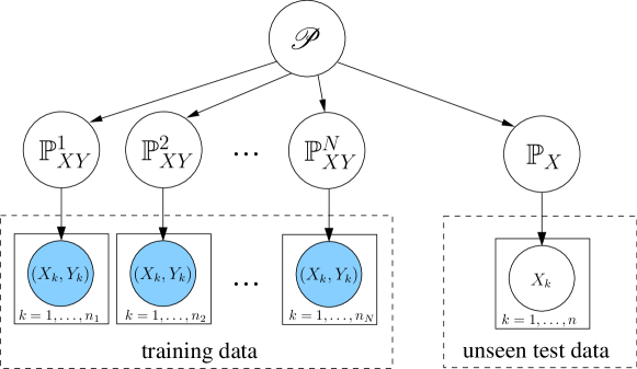
Figure 1. A simplified schematic diagram of the domain generalization framework. A major difference between our framework and most previous work in domain adaptation is that we do not observe the test domains during training time. See text for detailed description on how the data are generated.

1.1. Overview.

The goal of (supervised) domain generalization is to estimate a functional relationship that handles changes in the marginal $\mathbb{P}(X)$ or conditional $\mathbb{P}(Y|X)$ well, see Figure 1. We assume that the conditional probability $\mathbb{P}(Y|X)$ is stable or varies smoothly with the marginal $\mathbb{P}(X)$. Even if the conditional is stable, learning algorithms may still suffer from model misspecification due to variation in the marginal $\mathbb{P}(X)$. That is, if the learning algorithm cannot find a solution that perfectly captures the functional relationship between $X$ and $Y$ then its approximate solution will be sensitive to changes in $\mathbb{P}(X)$.

In this paper, we introduce Domain Invariant Component Analysis (DICA), a kernel-based algorithm that finds a transformation of the data that (i) minimizes the difference between marginal distributions $\mathbb{P}_{X}$ of domains as much as possible while (ii) preserving the functional relationship $\mathbb{P}(Y|X)$.

The novelty of this work is twofold. First, DICA extracts invariants: features that transfer across domains. It not only minimizes the divergence between marginal distributions $\mathbb{P}(X)$, but also preserves the functional relationship encoded in the posterior $\mathbb{P}(Y|X)$. The resulting learning algorithm is very simple. Second, while prior work in domain adaptation focused on using data from many different domains to specifically improve the performance on the target task, which is observed during the training time (the classifier is adapted to the specific target task), we assume access to abundant training data and are interested in the generalization ability of the invariant subspace to previously unseen domains (the classifier generalizes to new domains without retraining).

Moreover, we show that DICA generalizes or is closely related to many well-known dimension reduction algorithms including kernel principal component analysis (KPCA) (Schölkopf et al. 1998, Fukumizu et al. 2004a), transfer component analysis (TCA) (Pan et al. 2011), and covariance operator inverse regression (COIR) (Kim and Pavlovic 2011), see §2.5. The performance of DICA is analyzed theoretically §2.6 and demonstrated empirically §3.

1.2. Related work.

Domain generalization is a form of transfer learning, which applies expertise acquired in source domains to improve learning of target domains (cf. Pan and Yang (2010a) and references therein). Most previous work assumes the availability of the target domain to which the knowledge will be transferred. In contrast, domain generalization focuses on the generalization ability on previously unseen domains. That is, the test data comes from domains that are not available during training.

Recently, Blanchard et al. (2011) proposed an augmented SVM that incorporates empirical marginal distributions into the kernel. A detailed error analysis showed universal consistency of the approach. We apply methods from Blanchard et al. (2011) to derive theoretical guarantees on the finite sample performance of DICA.

Learning a shared subspace is a common approach in settings where there is distribution mismatch. For example, a typical approach in multitask learning is to uncover a joint (latent) feature/subspace that benefits tasks individually (Argyriou et al. 2007, Gu and Zhou 2009, Passos et al. 2012). A similar idea has been adopted in domain adaptation, where the learned subspace reduces mismatch between source and target domains (Gretton et al. 2009, Pan et al. 2011). Although these approaches have proven successful in various applications, no previous work has fully investigated the generalization ability of a subspace to unseen domains.

2. Domain-Invariant Component Analysis

Let $\mathcal{X}$ denote a nonempty input space and $\mathcal{Y}$ an arbitrary output space. We define a domain to be a joint distribution $\mathbb{P}_{XY}$ on $\mathcal{X}\times\mathcal{Y}$, and let $\mathfrak{P}_{\mathcal{X}\times\mathcal{Y}}$ denote the set of all domains. Let $\mathfrak{P}_{\mathcal{X}}$ and $\mathfrak{P}_{\mathcal{Y}|\mathcal{X}}$ denote the set of probability distributions $\mathbb{P}_{X}$ on $X$ and $\mathbb{P}_{Y|X}$ on $Y$ given $X$ respectively.

We assume domains are sampled from probability distribution $\mathscr{P}$ on $\mathfrak{P}_{\mathcal{X}\times\mathcal{Y}}$ which has a bounded second moment, i.e., the variance is well-defined. Domains are not observed directly. Instead, we observe $N$ samples $\mathcal{S}=\{S^{i}\}_{i=1}^{N}$, where $S^{i}=\{(x^{(i)}_{k},y^{(i)}_{k})\}_{k=1}^{n_{i}}$ is sampled from $\mathbb{P}^{i}_{XY}$ and each $\mathbb{P}^{1}_{XY},\ldots,\mathbb{P}^{N}_{XY}$ is sampled from $\mathscr{P}$. Since in general $\mathbb{P}_{XY}^{i}\neq\mathbb{P}_{XY}^{j}$, the samples in $\mathcal{S}$ are not i.i.d. Let $\widehat{\mathbb{P}}^{i}$ denote empirical distribution associated with each sample $S^{i}$. For brevity, we use $\mathbb{P}$ and $\mathbb{P}_{X}$ interchangeably to denote the marginal distribution.

Let $\mathcal{H}$ and $\mathcal{F}$ denote reproducing kernel Hilbert spaces (RKHSes) on $\mathcal{X}$ and $\mathcal{Y}$ with kernels $k:\mathcal{X}\times\mathcal{X}\rightarrow\mathbb{R}$ and $l:\mathcal{Y}\times\mathcal{Y}\rightarrow\mathbb{R}$, respectively. Associated with $\mathcal{H}$ and $\mathcal{F}$ are mappings $x\rightarrow\phi(x)\in\mathcal{H}$ and $y\rightarrow\varphi(y)\in\mathcal{F}$ induced by the kernels $k(\cdot,\cdot)$ and $l(\cdot,\cdot)$. Without loss of generality, we assume the feature maps of $X$ and $Y$ have zero means, i.e., $\sum_{k=1}^{n}\phi(x_{k})=0=\sum_{k=1}^{n}\varphi(y_{k})$. Let $\Sigma_{\mathrm{xx}}$, $\Sigma_{\mathrm{yy}}$, $\Sigma_{\mathrm{xy}}$, and $\Sigma_{\mathrm{yx}}$ be the covariance operators in and between the RKHSes of $X$ and $Y$.

2.1. Objective.

Using the samples $\mathcal{S}$, our goal is to produce an estimate $f:\mathfrak{P}_{\mathcal{X}}\times\mathcal{X}\rightarrow\mathbb{R}$ that generalizes well to test samples $S^{t}=\{x^{(t)}_{k}\}_{k=1}^{n_{t}}$ drawn according to some unknown distribution $\mathbb{P}^{t}\in\mathfrak{P}_{\mathcal{X}}$ (Blanchard et al. 2011). Since the performance of $f$ depends in part on how dissimilar the test distribution $\mathbb{P}^{t}$ is from those in the training samples, we propose to preprocess the data to actively reduce the dissimilarity between domains. Intuitively, we want to find transformation $\mathcal{B}$ in $\mathcal{H}$ that (i) minimizes the distance between empirical distributions of the transformed samples $\mathcal{B}(S^{i})$ and (ii) preserves the functional relationship between $X$ and $Y$, i.e., $Y\perp X\,|\,\mathcal{B}(X)$. We formulate an optimization problem capturing these constraints below.

2.2. Distributional Variance

First, we define the distributional variance, which measures the dissimilarity across domains. It is convenient to represent distributions as elements in an RKHS (Berlinet and Agnan 2004, Smola et al. 2007, Sriperumbudur et al. 2010) using the mean map

(1) $$\mu:\;\mathfrak{P}_{\mathcal{X}}\rightarrow\mathcal{H}:\;\mathbb{P}\mapsto\int_{\mathcal{X}}k(x,\cdot)\,\mathrm{d}\mathbb{P}(x)=:\mu_{\mathbb{P}}\enspace.$$

We assume that $k(x,x)$ is bounded for any $x\in\mathcal{X}$ such that $\mathbb{E}_{x\sim\mathbb{P}}[k(x,\cdot)]<\infty$. If $k$ is characteristic then (1) is injective, i.e., all the information about the distribution is preserved (Sriperumbudur et al. 2010). It also holds that $\mathbb{E}_{\mathbb{P}}[f]=\langle\mu_{\mathbb{P}},f\rangle_{\mathcal{H}}$ for all $f\in\mathcal{H}$ and any $\mathbb{P}$.

We decompose $\mathscr{P}$ into $\mathscr{P}_{X}$, which generates the marginal distribution $\mathbb{P}_{X}$, and $\mathscr{P}_{Y|X}$, which generates posteriors $\mathbb{P}_{Y|X}$. The data generating process begins by generating the marginal $\mathbb{P}_{X}$ according to $\mathscr{P}_{X}$. Conditioned on $\mathbb{P}_{X}$, it then generate conditional $\mathbb{P}_{Y|X}$ according to $\mathscr{P}_{Y|X}$. The data point $(x,y)$ is generated according to $\mathbb{P}_{X}$ and $\mathbb{P}_{Y|X}$, respectively. Given set of distributions ${\mathcal{P}}=\{\mathbb{P}^{1},\mathbb{P}^{2}\dotsc,\mathbb{P}^{N}\}$ drawn according to $\mathscr{P}_{X}$, define $N\times N$ Gram matrix $G$ with entries

(2) $$G_{ij}:=\langle\mu_{\mathbb{P}^{i}},\mu_{\mathbb{P}^{j}}\rangle_{\mathcal{H}}=\iint k(x,z)\,\mathrm{d}\mathbb{P}^{i}(x)\,\mathrm{d}\mathbb{P}^{j}(z),$$

for $i,j=1,\dotsc,N$. Note that $G_{ij}$ is the inner product between kernel mean embeddings of $\mathbb{P}^{i}$ and $\mathbb{P}^{j}$ in $\mathcal{H}$. Based on (2), we define the distributional variance, which estimates the variance of the distribution $\mathscr{P}_{X}$:

Definition 1.

Introduce probability distribution ${\mathcal{P}}$ on $\mathcal{H}$ with ${\mathcal{P}}(\mu_{\mathbb{P}^{i}})=\frac{1}{N}$ and center $G$ to obtain the covariance operator of ${\mathcal{P}}$, denoted as $\Sigma:=G-\mathbf{1}_{N}G-G\mathbf{1}_{N}+\mathbf{1}_{N}G\mathbf{1}_{N}$. The distributional variance is

(3) $${\mathbb{V}}_{\mathcal{H}}({\mathcal{P}}):=\frac{1}{N}\mathrm{tr}(\Sigma)=\frac{1}{N}\mathrm{tr}(G)-\dfrac{1}{N^{2}}\sum_{i,j=1}^{N}G_{ij}.$$

The following theorem shows that the distributional variance is suitable as a measure of divergence between domains.

Theorem 1.

Let $\bar{\mathbb{P}}=\frac{1}{N}\sum_{i=1}^{N}\mathbb{P}^{i}$. If $k$ is a characteristic kernel, then $\mathbb{V}_{\mathcal{H}}(\mathcal{P})=\frac{1}{N}\sum_{i=1}^{N}\lVert\mu_{\mathbb{P}^{i}}-\mu_{\bar{\mathbb{P}}}\rVert_{\mathcal{H}}^{2}=0$ if and only if $\mathbb{P}^{1}=\mathbb{P}^{2}=\cdots=\mathbb{P}^{N}$.

To estimate ${\mathbb{V}}_{\mathcal{H}}({\mathcal{P}})$ from $N$ sample sets $\mathcal{S}=\{S^{i}\}_{i=1}^{N}$ drawn from $\mathbb{P}^{1},\ldots,\mathbb{P}^{N}$, we define block kernel and coefficient matrices

$$K=\left(\begin{array}[]{cccc}K_{1,1}&\cdots&K_{1,N}\\ \vdots&\ddots&\vdots\\ K_{N,1}&\cdots&K_{N,N}\end{array}\right)\in\mathbb{R}^{n\times n}\enspace,Q=\left(\begin{array}[]{cccc}Q_{1,1}&\cdots&Q_{1,N}\\ \vdots&\ddots&\vdots\\ Q_{N,1}&\cdots&Q_{N,N}\end{array}\right)\in\mathbb{R}^{n\times n}\enspace,$$

where $n=\sum_{i=1}^{N}n_{i}$ and $[K_{i,j}]_{k,l}=k(x^{(i)}_{k},x^{(j)}_{l})$ is the Gram matrix evaluated between the sample $S^{i}$ and $S^{j}$. Following (3), elements of the coefficient matrix $Q_{i,j}\in\mathbb{R}^{n_{i}\times n_{j}}$ equal $(N-1)/(N^{2}n_{i}^{2})$ if $i=j$, and $-1/(N^{2}n_{i}n_{j})$ otherwise. Hence, the empirical distributional variance is

(4) $$\widehat{\mathbb{V}}_{\mathcal{H}}(\mathcal{S})=\frac{1}{N}\mathrm{tr}(\widehat{\Sigma})=\mathrm{tr}(KQ)\enspace.$$

Theorem 2.

The empirical estimator $\widehat{\mathbb{V}}_{\mathcal{H}}(\mathcal{S})=\frac{1}{N}\mathrm{tr}(\widehat{\Sigma})=\mathrm{tr}(KQ)$ obtained from Gram matrix

$$\widehat{G}_{ij}:=\dfrac{1}{n_{i}\cdot n_{j}}\sum_{k=1}^{n_{i}}\sum_{l=1}^{n_{j}}k(x^{(i)}_{k},x^{(j)}_{l})$$

is a consistent estimator of $\mathbb{V}_{\mathcal{H}}({\mathcal{P}})$.

2.3. Formulation of DICA

DICA finds an orthogonal transform $\mathcal{B}$ onto a low-dimensional subspace ($m\ll n$) that minimizes the distributional variance ${\mathbb{V}}_{\mathcal{H}}(\mathcal{S})$ between samples from $\mathcal{S}$, i.e. the dissimilarity across domains. Simultaneously, we require that $\mathcal{B}$ preserves the functional relationship between $X$ and $Y$, i.e. $Y\perp X\,|\,\mathcal{B}(X)$.

2.3.1. Minimizing distributional variance.

In order to simplify notation, we “flatten” $\{(x^{(i)}_{k},y^{(i)}_{k})_{k=1}^{n_{i}}\}_{i=1}^{N}$ to $\{(x_{k},y_{k})\}_{k=1}^{n}$ where $n=\sum_{i=1}^{N}n_{i}$. Let $\mathbf{b}_{k}=\sum_{i=1}^{n}\beta^{i}_{k}\phi(x_{i})=\Phi_{x}\bm{\beta}_{k}$ be the $k^{th}$ basis function of $\mathcal{B}$ where $\Phi_{x}=[\phi(x_{1}),\phi(x_{2}),\dotsc,\phi(x_{n})]$ and $\bm{\beta}_{k}$ are $n$-dimensional coefficient vectors. Let $B=[\bm{\beta}_{1},\bm{\beta}_{2},\ldots,\bm{\beta}_{m}]$ and $\tilde{\Phi}_{x}$ denote the projection of $\Phi_{x}$ onto $\mathbf{b}_{k}$, i.e., $\tilde{\Phi}_{x}=\mathbf{b}_{k}^{\top}\Phi_{x}=\bm{\beta}_{k}^{\top}\Phi_{x}^{\top}\Phi_{x}=\bm{\beta}_{k}^{\top}K$. The kernel on the $\mathcal{B}$-projection of $X$ is

(5) $$\widetilde{K}:=\tilde{\Phi}_{x}^{\top}\tilde{\Phi}_{x}=KBB^{\top}K\enspace.$$

After applying transformation $\mathcal{B}$, the empirical distributional variance between sample distributions is

(6) $$\widehat{\mathbb{V}}_{\mathcal{H}}(\mathcal{B}\mathcal{S})=\mathrm{tr}(\widetilde{K}Q)=\mathrm{tr}(B^{\top}KQKB)\enspace.$$

2.3.2. Preserving the functional relationship.

The central subspace $C$ is the minimal subspace that captures the functional relationship between $X$ and $Y$, i.e. $Y\perp X|C^{\top}X$. Note that in this work we generalize a linear transformation $C^{\top}X$ to nonlinear one $\mathcal{B}(X)$. To find the central subspace we use the inverse regression framework, (Li 1991):

Theorem 3.

If there exists a central subspace $C=[\mathbf{c}_{1},\ldots,\mathbf{c}_{m}]$ satisfying $Y\perp X|C^{\top}X$, and for any $a\in\mathbb{R}^{d}$, $\mathbb{E}[a^{\top}X|C^{\top}X]$ is linear in $\{\mathbf{c}^{\top}_{i}X\}_{i=1}^{m}$, then $\mathbb{E}[X|Y]\subset\text{span}\{\Sigma_{\mathrm{xx}}\mathbf{c}_{i}\}_{i=1}^{m}$.

It follows that the bases $C$ of the central subspace coincide with the $m$ largest eigenvectors of $\mathbb{V}(\mathbb{E}[X|Y])$ premultiplied by $\Sigma_{\mathrm{xx}}^{-1}$. Thus, the basis $\mathbf{c}$ is the solution to the eigenvalue problem $\mathbb{V}(\mathbb{E}[X|Y])\Sigma_{\mathrm{xx}}\mathbf{c}=\gamma\Sigma_{\mathrm{xx}}\mathbf{c}$. Alternatively, for each $\mathbf{c}_{k}$ one may solve

$$\underset{\mathbf{c}_{k}\in\mathbb{R}^{d}}{\text{max}}\;\frac{\mathbf{c}_{k}^{\top}\Sigma_{\mathrm{xx}}^{-1}\mathbb{V}(\mathbb{E}[X|Y])\Sigma_{\mathrm{xx}}\mathbf{c}_{k}}{\mathbf{c}_{k}^{\top}\mathbf{c}_{k}}$$

under the condition that $\mathbf{c}_{k}$ is chosen to not be in the span of the previously chosen $\mathbf{c}_{k}$. In our case, $x$ is mapped to $\phi(x)\in\mathcal{H}$ induced by the kernel $k$ and $\mathcal{B}$ has nonlinear basis functions $\mathbf{c}_{k}\in\mathcal{H},\,k=1,\ldots,m$. This nonlinear extension implies that $\mathbb{E}[X|Y]$ lies on a function space spanned by $\{\Sigma_{\mathrm{xx}}\mathbf{c}_{k}\}_{k=1}^{m}$, which coincide with the eigenfunctions of the operator $\mathbb{V}(\mathbb{E}[X|Y])$ (Wu 2008, Kim and Pavlovic 2011). Since we always work in $\mathcal{H}$, we drop $\phi$ from the notation below.

To avoid slicing the output space explicitly (Li 1991, Wu 2008), we exploit its kernel structure when estimating the covariance of the inverse regressor. The following result from Kim and Pavlovic (2011) states that, under a mild assumption, $\mathbb{V}(\mathbb{E}[X|Y])$ can be expressed in terms of covariance operators:

Theorem 4.

If for all $f\in\mathcal{H}$, there exists $g\in\mathcal{F}$ such that $\mathbb{E}[f(X)|y]=g(y)$ for almost every $y$, then

(7) $$\mathbb{V}(\mathbb{E}[X|Y])=\Sigma_{\mathrm{xy}}\Sigma_{\mathrm{yy}}^{-1}\Sigma_{\mathrm{yx}}\enspace.$$

Let $\Phi_{y}=[\varphi(y_{1}),\ldots,\varphi(y_{n})]$ and $L=\Phi_{y}^{\top}\Phi_{y}$. The covariance of inverse regressor (7) is estimated from the samples $\mathcal{S}$ as $\widehat{\mathbb{V}}(\mathbb{E}[X|Y])=\widehat{\Sigma}_{\mathrm{xy}}\widehat{\Sigma}_{\mathrm{yy}}^{-1}\widehat{\Sigma}_{\mathrm{yx}}=\frac{1}{n}\Phi_{x}L(L+n\varepsilon I_{n})^{-1}\Phi_{x}^{\top}$ where $\widehat{\Sigma}_{\mathrm{xy}}=\frac{1}{n}\Phi_{x}\Phi_{y}^{\top}$ and $\widehat{\Sigma}_{\mathrm{yy}}=\frac{1}{n}\Phi_{y}\Phi_{y}^{\top}$. Assuming inverses $\widehat{\Sigma}_{\mathrm{yy}}^{-1}$ and $\widehat{\Sigma}_{\mathrm{xx}}^{-1}$ exist, a straightforward computation (see Supplementary) shows

$$\mathbf{b}_{k}^{\top}\widehat{\Sigma}_{\mathrm{xx}}^{-1}\widehat{\mathbb{V}}(\mathbb{E}[X|Y])\widehat{\Sigma}_{\mathrm{xx}}\mathbf{b}_{k} = \frac{1}{n}\bm{\beta}_{k}^{\top}L(L+n\varepsilon I)^{-1}K^{2}\bm{\beta}_{k}$$

(8) $$\mathbf{b}_{k}^{\top}\mathbf{b}_{k} = \bm{\beta}_{k}^{\top}K\bm{\beta}_{k},$$

where $\varepsilon$ smoothes the affinity structure of the output space $Y$, thus acting as a kernel regularizer. Since we are interested in the projection of $\phi(x)$ onto the basis functions $\mathbf{b}_{k}$, we formulate the optimization in terms of $\bm{\beta}_{k}$. For a new test sample $x_{t}$, the projection onto basis function $\mathbf{b}_{k}$ is $\mathbf{k}_{t}\bm{\beta}_{k}$, where $\mathbf{k}_{t}=[k(x_{1},x_{t}),\ldots,k(x_{n},x_{t})]$.

2.3.3. The optimization problem.

Combining (6) and (8), DICA finds $B=[\bm{\beta}_{1},\bm{\beta}_{2},\ldots,\bm{\beta}_{m}]$ that solves

(9) $$\underset{B\in\mathbb{R}^{n\times m}}{\text{max}}\frac{\frac{1}{n}\mathrm{tr}\left(B^{\top}L(L+n\varepsilon I_{n})^{-1}K^{2}B\right)}{\mathrm{tr}\left(B^{\top}KQKB+BKB\right)}$$

The numerator requires that $B$ aligns with the bases of the central subspace. The denominator forces both dissimilarity across domains and the complexity of $B$ to be small, thereby tightening generalization bounds, see §2.6. Rewriting (9) as a constrained optimization (see Supplementary) yields Lagrangian

(10) $$\mathcal{L}= \frac{1}{n}\mathrm{tr}\left(B^{\top}L(L+n\varepsilon I_{n})^{-1}K^{2}B\right)-\mathrm{tr}\left(\left(B^{\top}KQKB+BKB-I_{m}\right)\Gamma\right)\enspace,$$

where $\Gamma$ is a diagonal matrix containing the Lagrange multipliers. Setting the derivative of (10) w.r.t. $B$ to zero yields the generalized eigenvalue problem:

(11) $$\frac{1}{n}L(L+n\varepsilon I_{n})^{-1}K^{2}B=(KQK+K)B\Gamma\enspace.$$

Transformation $B$ corresponds to the $m$ leading eigenvectors of the generalized eigenvalue problem (11).

The inverse regression framework based on covariance operators has two benefits. First, it avoids explicitly slicing the output space, which makes it suitable for high-dimensional output. Second, it allows for structured outputs on which explicit slicing may be impossible, e.g., trees and sequences. Since our framework is based entirely on kernels, it is applicable to any type of input and output variables, as long as the corresponding kernels can be defined.

2.4. Unsupervised DICA

In some application domains, such as image denoising, information about the target may not be available. We therefore derive an unsupervised version of DICA. Instead of preserving the central subspace, unsupervised DICA (UDICA) maximizes the variance of $X$ in the feature space, which is estimated as $\frac{1}{n}\mathrm{tr}(B^{\top}K^{2}B)$. Thus, UDICA solves

(12) $$\underset{B\in\mathbb{R}^{n\times m}}{\text{max}}\frac{\frac{1}{n}\mathrm{tr}(B^{\top}K^{2}B)}{\mathrm{tr}(B^{\top}KQKB+B^{\top}KB)}\enspace.$$

Similar to DICA, the solution of (12) is obtained by solving the generalized eigenvalue problem

(13) $$\frac{1}{n}K^{2}B=(KQK+K)B\Gamma\enspace.$$

UDICA is a special case of DICA where $L=\frac{1}{n}I$ and $\varepsilon\rightarrow 0$. Algorithm 1 summarizes supervised and unsupervised domain-invariant component analysis.

Algorithm 1 Domain-Invariant Component Analysis

Input:	Parameters $\lambda$, $\varepsilon$, and $m\ll n$. Sample $\mathcal{S}=\{S^{i}=\{(x_{k}^{(i)},y_{k}^{(i)})\}_{k=1}^{n_{i}}\}_{i=1}^{N}$.
Output:	Projection $B_{n\times m}$ and kernel $\widetilde{K}_{n\times n}$.

1:  Calculate gram matrix $[K_{ij}]_{kl}=k(x_{k}^{(i)},x_{l}^{(j)})$ and $[L_{ij}]_{kl}=l(y_{k}^{(i)},y_{l}^{(j)})$.

2:  Supervised: $C=L(L+n\varepsilon I)^{-1}K^{2}$.

3:  Unsupervised: $C=K^{2}$.

4:  Solve $\frac{1}{n}CB=(KQK+K+\lambda I)B\Gamma$ for $B$.

5:  Output $B$ and $\widetilde{K}\leftarrow KBB^{\top}K$.

6:  The test kernel $\widetilde{K}^{t}\leftarrow K^{t}BB^{\top}K$ where $K^{t}_{n_{t}\times n}$ is the joint kernel between test and training data.

2.5. Relations to Other Methods

The DICA and UDICA algorithms generalize many well-known dimension reduction techniques. In the supervised setting, if dataset $\mathcal{S}$ contains samples drawn from a single distribution $\mathbb{P}_{XY}$ then we have $KQK=\mathbf{0}$. Substituting $\alpha:=KB$ gives the eigenvalue problem $\frac{1}{n}L(L+n\varepsilon I)^{-1}K\alpha=K\alpha\Gamma$, which corresponds to covariance operator inverse regression (COIR) (Kim and Pavlovic 2011).

If there is only a single distribution then unsupervised DICA reduces to KPCA since $KQK=\mathbf{0}$ and finding $B$ requires solving the eigensystem $KB=B\Gamma$ which recovers KPCA (Schölkopf et al. 1998). If there are two domains, source $\mathbb{P}_{S}$ and target $\mathbb{P}_{T}$, then UDICA is closely related – though not identical to – Transfer Component Analysis (Pan et al. 2011). This follows from the observation that $\mathbb{V}_{\mathcal{H}}(\{\mathbb{P}_{S},\mathbb{P}_{T}\})=\|\mu_{\mathbb{P}_{S}}-\mu_{\mathbb{P}_{T}}\|^{2}$, see proof of Theorem 1.

2.6. A Learning-Theoretic Bound

We bound the generalization error of a classifier trained after DICA-preprocessing. The main complication is that samples are not identically distributed. We adapt an approach to this problem developed in Blanchard et al. (2011) to prove a generalization bound that applies after transforming the empirical sample using $\mathcal{B}$. Recall that $\mathcal{B}=\Phi_{x}B$.

Define kernel $\bar{k}$ on $\mathfrak{P}\times\mathcal{X}$ as $\bar{k}((\mathbb{P},x),(\mathbb{P}^{\prime},x^{\prime})):=k_{\mathfrak{P}}(\mathbb{P},\mathbb{P}^{\prime})\cdot k_{\mathcal{X}}(x,x^{\prime})$. Here, $k_{\mathcal{X}}$ is the kernel on $\mathcal{H}_{\mathcal{X}}$ and the kernel on distributions is $k_{\mathfrak{P}}(\mathbb{P},\mathbb{P}^{\prime}):=\kappa(\mu_{\mathbb{P}},\mu_{\mathbb{P}^{\prime}})$ where $\kappa$ is a positive definite kernel (Christmann and Steinwart 2010, Muandet et al. 2012). Let $\Psi_{\mathfrak{P}}$ denote the corresponding feature map.

Theorem 5.

Under reasonable technical assumptions, see Supplementary, it holds with probability at least $1-\delta$ that,

$$\sup_{\|f\|_{\mathcal{H}}\leq 1}\left|\mathbb{E}_{\mathscr{P}}^{*}\mathbb{E}_{\mathbb{P}}\ell(f(\tilde{X}_{ij}\mathcal{B}),Y_{i})-\mathbb{E}_{\hat{\mathbb{P}}}\ell(f(\tilde{X}_{ij}\mathcal{B}),Y_{i})\right|^{2}$$

$$\leq c_{1}\frac{1}{N}\mathrm{tr}(B^{\intercal}KQKB)+\mathrm{tr}(B^{\top}KB)\left(c_{2}\frac{N(\log\frac{1}{\delta}+2\log N)}{n}+\frac{c_{3}\log\frac{1}{\delta}+c_{4}}{N}\right).$$

The LHS is the difference between the training error and expected error (with respect to the distribution on domains $\mathscr{P}^{*}$) after applying $\mathcal{B}$.

The first term in the bound, involving $\text{tr}(B^{\intercal}KQKB)$, quantifies the distributional variance after applying the transform: the higher the distributional variance, the worse the guarantee, tying in with analogous results in Ben-David et al. (2007; 2010). The second term in the bound depends on the size of the distortion ${\rm tr}(B^{\intercal}KB)$ introduced by $B$: the more complicated the transform, the worse the guarantee.

The bound reveals a tradeoff between reducing the distributional variance and the complexity or size of the transform used to do so. The denominator of (9) is a sum of these terms, so that DICA tightens the bound in Theorem 5.

Preserving the functional relationship (i.e. central subspace) by maximizing the numerator in (9) should reduce the empirical risk $\mathbb{E}_{\hat{\mathbb{P}}}\ell(f(\tilde{X}_{ij}\mathcal{B}),Y_{i})$. However, a rigorous demonstration has yet to be found.

3. Experiments

We illustrate the difference between the proposed algorithms and their single-domain counterparts using a synthetic dataset. Furthermore, we evaluate DICA in two tasks: a classification task on flow cytometry data and a regression task for Parkinson’s telemonitoring.

3.1. Toy Experiments

We generate 10 collections of $n_{i}\sim\mathtt{Poisson}(200)$ data points. The data in each collection is generated according to a five-dimensional zero-mean Gaussian distribution. For each collection, the covariance of the distribution is generated from Wishart distribution $\mathcal{W}(0.2\times I_{5},10)$. This step is to simulate different marginal distributions. The output value is $y=\mathrm{sign}(b_{1}^{\top}x+\epsilon_{1})\cdot\log(\lvert b_{2}^{\top}x+c+\epsilon_{2}\rvert)$, where $b_{1},b_{2}$ are the weight vectors, $c$ is a constant, and $\epsilon_{1},\epsilon_{2}\sim\mathcal{N}(0,1)$. Note that $b_{1}$ and $b_{2}$ form a low-dimensional subspace that captures the functional relationship between $X$ and $Y$. We then apply the KPCA, UDICA, COIR, and DICA algorithms on the dataset with Gaussian RBF kernels for both $X$ and $Y$ with bandwidth parameters $\sigma_{x}=\sigma_{y}=1$, $\lambda=0.1$, and $\varepsilon=10^{-4}$.

Fig. 2 shows projections of the training and three previously unseen test datasets onto the first two eigenvectors. The subspaces obtained from UDICA and DICA are more stable than for KPCA and COIR. In particular, COIR shows a substantial difference between training and test data, suggesting overfitting.

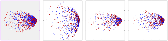
KPCA

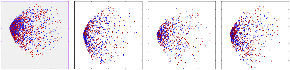
UDICA

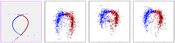
COIR

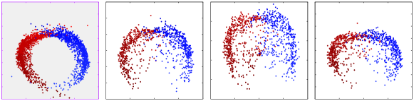
DICA

Figure 2. Projections of a synthetic dataset onto the first two eigenvectors obtained from the KPCA, UDICA, COIR, and DICA. The colors of data points corresponds to the output values. The shaded boxes depict the projection of training data, whereas the unshaded boxes show projections of unseen test datasets. The feature representations learnt by UDICA and DICA are more stable across test domains than those learnt by KPCA and COIR.

3.2. Gating of Flow Cytometry Data

Graft-versus-host disease (GvHD) occurs in allogeneic hematopoietic stem cell transplant recipients when donor-immune cells in the graft recognize the recipient as “foreign” and initiate an attack on the skin, gut, liver, and other tissues. It is a significant clinical problem in the field of allogeneic blood and marrow transplantation. The GvHD dataset (Brinkman et al. 2007) consists of weekly peripheral blood samples obtained from 31 patients following allogenic blood and marrow transplant. The goal of gating is to identify $\mbox{CD}3^{+}\mbox{CD}4^{+}\mbox{CD}8\beta^{+}$ cells, which were found to have a high correlation with the development of GvHD (Brinkman et al. 2007). We expect to find a subspace of cells that is consistent to the biological variation between patients, and is indicative of the GvHD development. For each patient, we select a dataset that contains sufficient numbers of the target cell populations. As a result, we omit one patient due to insufficient data. The corresponding flow cytometry datasets from 30 patients have sample sizes ranging from 1,000 to 10,000, and the proportion of the $\mbox{CD}3^{+}\mbox{CD}4^{+}\mbox{CD}8\beta^{+}$ cells in each dataset ranges from 10% to 30%, depending on the development of the GvHD.

Table 1. Average accuracies over 30 random subsamples of GvHD datasets. Pooling SVM applies standard kernel function on the pooled data from multiple domains, whereas distributional SVM also considers similarity between domains using kernel (14). With sufficiently many samples, DICA outperforms other methods in both pooling and distributional settings. The performance of pooling SVM and distributional SVM are comparable in this case.

Methods	Pooling SVM			Distributional SVM
	$n_{i}=100$	$n_{i}=500$	$n_{i}=1000$	$n_{i}=100$	$n_{i}=500$	$n_{i}=1000$
Input	91.68$\pm$.91	92.11$\pm$1.14	93.57$\pm$.77	91.53$\pm$.76	92.81$\pm$.93	92.41$\pm$.98
KPCA	91.65$\pm$.93	92.06$\pm$1.15	93.59$\pm$.77	91.83$\pm$.60	90.86$\pm$1.98	92.61$\pm$1.12
COIR	91.71$\pm$.88	92.00$\pm$1.05	92.57$\pm$.97	91.42$\pm$.95	91.54$\pm$1.14	92.61$\pm$.89
UDICA	91.20$\pm$.81	92.21$\pm$.19	93.02$\pm$.77	91.51$\pm$.79	91.74$\pm$1.08	93.02$\pm$.77
DICA	91.37$\pm$.91	92.71$\pm$.82	94.16$\pm$.73	91.51$\pm$.89	93.42$\pm$.73	93.33$\pm$.86

To evaluate the performance of the proposed algorithms, we took data from $N=10$ patients for training, and the remaining 20 patients for testing. We subsample the training sets and test sets to have 100, 500, and 1,000 data points (cells) each. We compare the SVM classifiers under two settings, namely, a pooling SVM and a distributional SVM. The pooling SVM disregards the inter-patient variation by combining all datasets from different patients, whereas the distributional SVM also takes the inter-patient variation into account via the kernel function (Blanchard et al. 2011)

(14) $$K(\tilde{x}^{(i)}_{k},\tilde{x}^{(j)}_{l})=k_{1}(\mathbb{P}^{i},\mathbb{P}^{j})\cdot k_{2}(x_{k}^{(i)},x_{l}^{(j)})$$

where $\tilde{x}^{(i)}_{k}=(\mathbb{P}^{i},x_{k}^{(i)})$ and $k_{1}$ is the kernel on distributions. We use $k_{1}(\mathbb{P}^{i},\mathbb{P}^{j})=\exp\left(-\|\mu_{\mathbb{P}^{i}}-\mu_{\mathbb{P}^{j}}\|^{2}_{\mathcal{H}}/2\sigma_{1}^{2}\right)$ and $k_{2}(x_{k}^{(i)},x_{l}^{(j)})=\exp(-\|x_{k}^{(i)}-x_{l}^{(j)}\|^{2}/2\sigma_{2}^{2})$, where $\mu_{\mathbb{P}^{i}}$ is computed using $k_{2}$. For pooling SVM, the kernel $k_{1}(\mathbb{P}^{i},\mathbb{P}^{j})$ is constant for any $i$ and $j$. Moreover, we use the output kernel $l(y^{(i)}_{k},y^{(j)}_{l})=\delta(y^{(i)}_{k},y^{(j)}_{l})$ where $\delta(a,b)$ is 1 if $a=b$, and 0 otherwise. We compare the performance of the SVMs trained on the preprocessed datasets using the KPCA, COIR, UDICA, and DICA algorithms. It is important to note that we are not defining another kernel on top of the preprocessed data. That is, the kernel $k_{2}$ for KPCA, COIR, UDICA, and DICA is exactly (5). We perform 10-fold cross validation on the parameter grids to optimize for accuracy.

Table 2. The average leave-one-out accuracies over 30 subjects on GvHD data. The distributional SVM outperforms the pooling SVM. DICA improves classifier accuracy.

Methods	Pooling SVM	Distributional SVM
Input	92.03$\pm$8.21	93.19$\pm$7.20
KPCA	91.99$\pm$9.02	93.11$\pm$6.83
COIR	92.40$\pm$8.63	92.92$\pm$8.20
UDICA	92.51$\pm$5.09	92.74$\pm$5.01
DICA	92.72$\pm$6.41	94.80$\pm$3.81

Table 1 reports average accuracies and their standard deviation over 30 repetitions of the experiments. For sufficiently large number of samples, DICA outperforms other approaches. The pooling SVM and distributional SVM achieve comparable accuracies. The average leave-one-out accuracies over 30 subjects are reported in Table 2 (see supplementary for more detail).

3.3. Parkinson’s Telemonitoring

To evaluate DICA in a regression setting, we apply it to a Parkinson’s telemonitoring dataset. The dataset consists of biomedical voice measurements from 42 people with early-stage Parkinson’s disease recruited for a six-month trial of a telemonitoring device for remote symptom progression monitoring. The aim is to predict the clinician’s motor and total UPDRS scoring of Parkinson’s disease symptoms from 16 voice measures. There are around 200 recordings per patient.

Table 3. Root mean square error (RMSE) of the independent Gaussian Process regression (GPR) applied to the Parkinson’s telemonitoring dataset. DICA outperforms other approaches in both settings; and the distributional SVM outperforms the pooling SVM.

Methods	Pooling GP Regression		Distributional GP Regression
	motor score	total score	motor score	total score
LLS	8.82 $\pm$ 0.77	11.80 $\pm$ 1.54	8.82 $\pm$ 0.77	11.80 $\pm$ 1.54
Input	9.58 $\pm$ 1.06	12.67 $\pm$ 1.40	8.57 $\pm$ 0.77	11.50 $\pm$ 1.56
KPCA	8.54 $\pm$ 0.89	11.20 $\pm$ 1.47	8.50 $\pm$ 0.87	11.22 $\pm$ 1.49
UDICA	8.67 $\pm$ 0.83	11.36 $\pm$ 1.43	8.75 $\pm$ 0.97	11.55 $\pm$ 1.52
COIR	9.25 $\pm$ 0.75	12.41 $\pm$ 1.63	9.23 $\pm$ 0.90	11.97 $\pm$ 2.09
DICA	8.40 $\pm$ 0.76	11.05 $\pm$ 1.50	8.35 $\pm$ 0.82	10.02 $\pm$ 1.01

We adopt the same experimental settings as in §3.2, except that we employ two independent Gaussian Process (GP) regression to predict motor and total UPDRS scores. For COIR and DICA, we consider the output kernel $l(y^{(i)}_{k},y^{(j)}_{l})=\exp(-\|y^{(i)}_{k}-y^{(j)}_{l}\|^{2}/2\sigma_{3}^{2})$ to fully account for the affinity structure of the output variable. We set $\sigma_{3}$ to be the median of motor and total UPDRS scores. The voice measurements from 30 patients are used for training and the rest for testing.

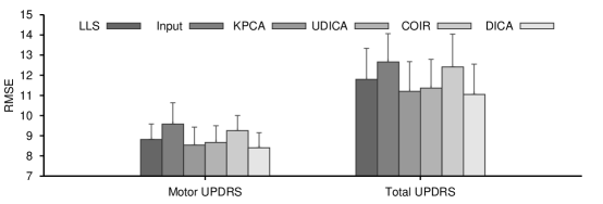
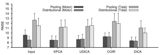
Figure 3. The root mean square error (RMSE) of motor and total UPDRS scores predicted by GP regression after different preprocessing methods on Parkinson’s telemonitoring dataset. The top and middle rows depicts the pooling and distributional settings; the bottom row compares the two settings. Results of linear least square (LLS) are given as a baseline.

Fig. 3 depicts the results. DICA consistently, though not statistically significantly, outperforms other approaches, see Table 3. Inter-patient (i.e. across domain) variation worsens prediction accuracy on new patients. Reducing this variation with DICA improves the accuracy on new patients. Moreover, incorporating the inter-subject variation via distributional GP regression further improves the generalization ability, see Fig. 3.

4. Conclusion and Discussion

To conclude, we proposed a simple algorithm called Domain-Invariant Component Analysis (DICA) for learning an invariant transformation of the data which has proven significant for domain generalization both theoretically and empirically. Theorem 5 shows the generalization error on previously unseen domains grows with the distributional variance. We also showed that DICA generalizes KPCA and COIR, and is closely related to TCA. Finally, experimental results on both synthetic and real-world datasets show DICA performs well in practice. Interestingly, the results also suggest that the distributional SVM, which takes into account inter-domain variation, outperforms the pooling SVM which ignores it.

The motivating assumption in this work is that the functional relationship is stable or varies smoothly across domains. This is a reasonable assumption for automatic gating of flow cytometry data because the inter-subject variation of cell population makes it impossible for domain expert to apply the same gating on all subjects, and similarly makes sense for Parkinson’s telemonitoring data. Nevertheless, the assumption does not hold in many applications where the conditional distributions are substantially different. It remains unclear how to develop techniques that generalize to previously unseen domains in these scenarios.

DICA can be adapted to novel applications by equipping the optimization problem with appropriate constraints. For example, one can formulate a semi-supervised extension of DICA by forcing the invariant basis functions to lie on a manifold or preserve a neighborhood structure. Moreover, by incorporating the distributional variance as a regularizer in the objective function, the invariant features and classifier can be optimized simultaneously.

Acknowledgments

We thank Samory Kpotufe and Kun Zhang for fruitful discussions and the three anonymous reviewers for insightful comments and suggestions that significantly improved the paper.

Appendix A Domain Generalization and Related Frameworks

The most fundamental assumption in machine learning is that the observations are independent and identically distributed (i.i.d.). That is, each observation comes from the same probability distribution as the others and all are mutually independent. However, this assumption is often violated in practice, in which case the standard machine learning algorithms do not perform well. In the past decades, many techniques have been proposed to tackle scenarios where there is a mismatch between training and test distributions. These include domain adaptation [Bickel et al., 2009a], multitask learning [Caruana, 1997], transfer learning [Pan and Yang, 2010b], covariate/dataset shift [Quionero-Candela et al., 2009] and concept drift [Widmer and Kurat, 1996]. To better understand domain generalization, we briefly discuss how it relates to some of these approaches.

A.1. Transfer learning (see e.g., Pan and Yang [2010b] and references therein).

Transfer learning aims at transferring knowledge from some previous tasks to a target task when the latter has limited training data. That is, although there may be few labeled examples, “knowledge” obtained in related tasks may be available. Transfer learning focuses on improving the learning of the target predictive function using the knowledge in the source task. Although not identical, domain generalization can be viewed as a transfer learning when knowledge of the target task is unavailable during training.

A.2. Multitask learning (see e.g., Caruana [1997] and references therein).

The goal of multitask learning is to learn multiple tasks simultaneously – especially when training examples in each task are scarce. By learning all tasks simultaneously, one expects to improve generalization on individual tasks. An important assumption is therefore that all the tasks are related. Multitask learning differs from domain generalization because learning the new task often requires retraining.

A.3. Domain adaptation (see e.g., Bickel et al. [2009a] and references therein).

Domain adaptation, also known as covariate shift, deals primarily with a mismatch between training and test distributions. Domain generalization deals with a broader setting where training instances may have been collected from multiple source domains. A second difference is that in domain adaptation one observes the target domain during the training time whereas in domain generalization one does not.

Table 4 summarizes the main differences between the various frameworks.

Table 4. Comparison of domain generalization with other well-known frameworks. Note that the domain generalization is closely related to multi-task learning and domain adaptation. The difference of domain generalization is that one does not observe the target domains in which a classifier will be applied without retraining the classifier.

Framework	Distribution Mismatch	Multiple Sources	Target Domain
Standard Setup	✗	✗	✗
Transfer Learning	✓	✗	✓
Multi-task Learning	✓	✓	✗
Domain Adaptation	✓	✓	✓
Domain Generalization	✓	✓	✗

Appendix B Proof of Theorem 1

Lemma 6.

Given a set of distributions $\mathcal{P}=\{\mathbb{P}^{1},\mathbb{P}^{2}\dotsc,\mathbb{P}^{N}\}$, the distributional variance of $\mathcal{P}$ is $\mathbb{V}_{\mathcal{H}}(\mathcal{P})=\frac{1}{N}\sum_{i=1}^{N}\lVert\mu_{\mathbb{P}^{i}}-\mu_{\bar{\mathbb{P}}}\rVert_{\mathcal{H}}^{2}$ where $\mu_{\bar{\mathbb{P}}}=(1/N)\sum_{i=1}^{N}\mu_{\mathbb{P}^{i}}$ and $\bar{\mathbb{P}}=\frac{1}{N}\sum_{i=1}^{N}\mathbb{P}^{i}$.

Proof.

Let $\bar{\mathbb{P}}$ be the probability distribution defined as $(1/N)\sum_{i=1}^{N}\mathbb{P}^{i}$, i.e., $\bar{\mathbb{P}}(x)=(1/N)\sum_{i=1}^{N}\mathbb{P}^{i}(x)$. It follows from the linearity of the expectation that $\mu_{\bar{\mathbb{P}}}=(1/N)\sum_{i=1}^{N}\mu_{\mathbb{P}^{i}}$. For brevity, we will denote $\langle\cdot,\cdot\rangle_{\mathcal{H}}$ by $\langle\cdot,\cdot\rangle$. Then, expanding (3) gives

$$\mathbb{V}_{\mathcal{H}}(\mathcal{P}) = \frac{1}{N}\mathrm{tr}(\Sigma)=\frac{1}{N}\text{tr}(G)-\dfrac{1}{N^{2}}\sum_{i,j=1}^{N}G_{ij}$$

$$= \frac{1}{N}\sum_{i=1}^{N}\langle\mu_{\mathbb{P}^{i}},\mu_{\mathbb{P}^{i}}\rangle-\frac{1}{N^{2}}\sum_{i,j=1}^{N}\langle\mu_{\mathbb{P}^{i}},\mu_{\mathbb{P}^{j}}\rangle$$

$$= \frac{1}{N}\left[\sum_{i=1}^{N}\langle\mu_{\mathbb{P}^{i}},\mu_{\mathbb{P}^{i}}\rangle-\frac{2}{N}\sum_{i,j=1}^{N}\langle\mu_{\mathbb{P}^{i}},\mu_{\mathbb{P}^{j}}\rangle+\frac{1}{N}\sum_{i,j=1}^{N}\langle\mu_{\mathbb{P}^{i}},\mu_{\mathbb{P}^{j}}\rangle\right]$$

$$= \frac{1}{N}\left[\sum_{i=1}^{N}\langle\mu_{\mathbb{P}^{i}},\mu_{\mathbb{P}^{i}}\rangle-2\sum_{i=1}^{N}\left\langle\mu_{\mathbb{P}^{i}},\frac{1}{N}\sum_{j=1}^{N}\mu_{\mathbb{P}^{j}}\right\rangle+N\left\langle\frac{1}{N}\sum_{i=1}^{N}\mu_{\mathbb{P}^{i}},\frac{1}{N}\sum_{j=1}^{N}\mu_{\mathbb{P}^{j}}\right\rangle\right]$$

$$= \frac{1}{N}\left[\sum_{i=1}^{N}\langle\mu_{\mathbb{P}^{i}},\mu_{\mathbb{P}^{i}}\rangle-2\sum_{i=1}^{N}\langle\mu_{\mathbb{P}^{i}},\mu_{\bar{\mathbb{P}}}\rangle+N\langle\mu_{\bar{\mathbb{P}}},\mu_{\bar{\mathbb{P}}}\rangle\right]$$

$$= \frac{1}{N}\sum_{i=1}^{N}\Big{(}\langle\mu_{\mathbb{P}^{i}},\mu_{\mathbb{P}^{i}}\rangle-2\cdot\langle\mu_{\mathbb{P}^{i}},\mu_{\bar{\mathbb{P}}}\rangle+\langle\mu_{\bar{\mathbb{P}}},\mu_{\bar{\mathbb{P}}}\rangle\Big{)}$$

$$= \frac{1}{N}\sum_{i=1}^{N}\lVert\mu_{\mathbb{P}^{i}}-\mu_{\bar{\mathbb{P}}}\rVert_{\mathcal{H}}^{2}\enspace,$$

which completes the proof. ∎

• For a characteristic kernel $k$, $\mathbb{V}_{\mathcal{H}}(\mathcal{P})=0$ if and only if $\mathbb{P}^{1}=\mathbb{P}^{2}=\cdots=\mathbb{P}^{N}$.

Proof.

Since $k$ is characteristic, $\lVert\mu_{\mathbb{P}}-\mu_{\mathbb{Q}}\rVert^{2}_{\mathcal{H}}$ is a metric and is zero iff $\mathbb{P}=\mathbb{Q}$ for any distributions $\mathbb{P}$ and $\mathbb{Q}$ [Sriperumbudur et al., 2010]. By Lemma 6, $\mathbb{V}_{\mathcal{H}}(\mathcal{P})=\frac{1}{N}\sum_{i=1}^{N}\lVert\mu_{\mathbb{P}^{i}}-\mu_{\bar{\mathbb{P}}}\rVert_{\mathcal{H}}^{2}.$ Thus, $\lVert\mu_{\mathbb{P}^{i}}-\mu_{\bar{\mathbb{P}}}\rVert_{\mathcal{H}}^{2}=0$ iff $\mathbb{P}^{i}=\bar{\mathbb{P}}$. Consequently, if $\mathbb{V}_{\mathcal{H}}(\mathcal{P})$ is zero, this implies that $\mathbb{P}^{i}=\bar{\mathbb{P}}$ for all $i$, meaning that $\mathbb{P}^{1}=\cdots=\mathbb{P}^{\ell}$. Conversely, if $\mathbb{P}^{1}=\cdots=\mathbb{P}^{\ell}$, then $\lVert\mu_{\mathbb{P}^{i}}-\mu_{\bar{\mathbb{P}}}\rVert_{\mathcal{H}}^{2}=0$ is zero for all $i$ and thereby $\mathbb{V}_{\mathcal{H}}(\mathcal{P})=\frac{1}{N}\sum_{i=1}^{N}\lVert\mu_{\mathbb{P}^{i}}-\mu_{\bar{\mathbb{P}}}\rVert_{\mathcal{H}}^{2}$ is zero. ∎

Appendix C Proof of Theorem 2

• The empirical estimator $\widehat{\mathbb{V}}_{\mathcal{H}}(\mathcal{S})=\frac{1}{N}\mathrm{tr}(\widehat{\Sigma})=\mathrm{tr}(KQ)$ obtained from Gram matrix

  $$\widehat{G}_{ij}:=\dfrac{1}{n_{i}\cdot n_{j}}\sum_{k=1}^{n_{i}}\sum_{l=1}^{n_{j}}k(x^{(i)}_{k},x^{(j)}_{l})$$

  is a consistent estimator of $\mathbb{V}_{\mathcal{H}}({\mathcal{P}})$.

Proof.

Recall that

$$\mathbb{V}_{\mathcal{H}}(\mathcal{P})=\frac{1}{N}\mathrm{tr}(G)-\frac{1}{N^{2}}\sum_{i,j=1}^{N}G_{ij}\enspace\text{ and }\enspace\widehat{\mathbb{V}}_{\mathcal{H}}(\mathcal{S})=\frac{1}{N}\mathrm{tr}(\widehat{G})-\frac{1}{N^{2}}\sum_{i,j=1}^{N}\widehat{G}_{ij}$$

where

$$G_{ij} = \langle\mu_{\mathbb{P}^{i}},\mu_{\mathbb{P}^{j}}\rangle_{\mathcal{H}}=\iint k(x,z)\,\mathrm{d}\mathbb{P}^{i}(x)\,\mathrm{d}\mathbb{P}^{j}(z)$$

$$\widehat{G}_{ij} = \langle\hat{\mu}_{\mathbb{P}^{i}},\hat{\mu}_{\mathbb{P}^{j}}\rangle_{\mathcal{H}}=\frac{1}{n_{i}n_{j}}\sum_{k=1}^{n_{i}}\sum_{l=1}^{n_{j}}k(x_{k}^{(i)},x_{l}^{(j)})$$

By Theorem 15 in Altun and Smola [2006], we have a fast convergence of $\hat{\mu}_{\mathbb{P}}$ to $\mu_{\mathbb{P}}$. Consequently, we have $\widehat{G}\rightarrow G$, which implies that $\widehat{\mathbb{V}}_{\mathcal{H}}(\mathcal{S})\rightarrow\mathbb{V}_{\mathcal{H}}(\mathcal{P})$. Hence, $\widehat{\mathbb{V}}_{\mathcal{H}}(\mathcal{S})$ is a consistent estimator of $\mathbb{V}_{\mathcal{H}}(\mathcal{P})$. ∎

Appendix D Derivation of Eq. (8)

DICA employs the covariance of inverse regressor $\mathbb{V}(\mathbb{E}[\phi(X)|Y])$, which can be written in terms of covariance operators. Let $\mathcal{H}$ and $\mathcal{F}$ be the RKHSes of $X$ and $Y$ endowed with reproducing kernels $k$ and $l$, respectively. Let $\Sigma_{\mathrm{xx}}$, $\Sigma_{\mathrm{yy}}$, $\Sigma_{\mathrm{xy}}$, and $\Sigma_{\mathrm{yx}}$ be the covariance operators in and between the corresponding RKHSes of $X$ and $Y$. We define the conditional covariance operator of $X$ given $Y$, denoted by $\Sigma_{\mathrm{xx}|\mathrm{y}}$, as

(15) $$\Sigma_{\mathrm{xx}|\mathrm{y}}\triangleq\Sigma_{\mathrm{xx}}-\Sigma_{\mathrm{xy}}\Sigma_{\mathrm{yy}}^{-1}\Sigma_{\mathrm{yx}}\enspace.$$

The following theorem from Fukumizu et al. [2004b] states that, under mild conditions, $\Sigma_{\mathrm{xx}|\mathrm{y}}$ equals the expected conditional variance of $\phi(X)$ given $Y$.

Theorem 7.

For any $f\in\mathcal{H}$, if there exists $g\in\mathcal{F}$ such that $\mathbb{E}[f(X)|Y]=g(Y)$ for almost every $Y$, then $\Sigma_{\mathrm{xx}|\mathrm{y}}=\mathbb{E}[\mathbb{V}(\phi(X)|Y)]$.

Using the $E\text{-}V\text{-}V\text{-}E$ identity, the covariance $\mathbb{V}(\mathbb{E}[\phi(X)|Y])$ can be expressed in terms of the conditional covariance operators as follow:

(16) $$\mathbb{V}(\mathbb{E}[\phi(X)|Y])=\mathbb{V}(\phi(X))-\mathbb{E}[\mathbb{V}(\phi(X)|Y)],$$

assuming that the inverse regressor $\mathbb{E}[f(x)|y]$ is a smooth function of $y$ for any $f\in\mathcal{H}$.

By virtue of Theorem 7, the second term in the r.h.s. of (16) is $\Sigma_{\mathrm{xx}|\mathrm{y}}$. Since $\mathbb{V}(\phi(X))=\mathrm{Cov}(\phi(x),\phi(x))=\Sigma_{\mathrm{xx}}$, it follows from (15) that the covariance of the inverse regression $\mathbb{V}(\mathbb{E}[\phi(X)]|Y)$ can be expressed as

(17) $$\mathbb{V}(\mathbb{E}[\phi(X)|Y])=\Sigma_{\mathrm{xy}}\Sigma_{\mathrm{yy}}^{-1}\Sigma_{\mathrm{yx}}\enspace.$$

The covariance (17) can be estimated from finite samples $(x_{1},y_{1}),\dotsc,(x_{n},y_{n})$ by $\widehat{\mathbb{V}}(\mathbb{E}[\phi(X)|Y])=\widehat{\Sigma}_{\mathrm{xy}}\widehat{\Sigma}_{\mathrm{yy}}^{-1}\widehat{\Sigma}_{\mathrm{yx}}$ where $\widehat{\Sigma}_{\mathrm{xy}}=\frac{1}{n}\Phi_{x}\Phi_{y}^{\top}$ and $\Phi_{x}=[\phi(x_{1}),\dotsc,\phi(x_{n})]$ and $\Phi_{y}=[\varphi(y_{1}),\dotsc,\varphi(y_{n})]$. Let $K$ and $L$ denote the kernel matrices computed over samples $\{x_{1},x_{2},\dotsc,x_{n}\}$ and $\{y_{1},y_{2},\dotsc,y_{n}\}$, respectively. We have

$$\widehat{\mathbb{V}}(\mathbb{E}[\phi(X)|Y]) =\left(\frac{1}{n}\Phi_{x}\Phi_{y}^{\top}\right)\left(\frac{1}{n}(\Phi_{y}\Phi_{y}^{\top}+n\varepsilon\mathcal{I})\right)^{-1}\left(\frac{1}{n}\Phi_{y}\Phi_{x}^{\top}\right)$$

$$=\frac{1}{n}\Phi_{x}\Phi_{y}^{\top}\Phi_{y}\left(\Phi_{y}^{\top}\Phi_{y}+n\varepsilon I_{n}\right)^{-1}\Phi_{x}^{\top}$$

(18) $$=\frac{1}{n}\Phi_{x}L\left(L+n\varepsilon I_{n}\right)^{-1}\Phi_{x}^{\top}$$

where $L=\Phi_{y}^{\top}\Phi_{y}$ and $\mathcal{I}$ is the identity operator. The second equation is obtained by applying the fact that $(\Phi_{y}\Phi_{y}^{\top}+n\varepsilon\mathcal{I})\Phi_{y}=\Phi_{y}(\Phi_{y}^{\top}\Phi_{y}+n\varepsilon I_{n})$.

Finally, using $\widehat{\Sigma}_{\mathrm{xx}}=\frac{1}{n}\Phi_{x}\Phi_{x}^{\top}$ and recalling that $K=\Phi_{x}^{\top}\Phi_{x}$, we obtain

$$\mathbf{b}_{k}^{\top}\widehat{\Sigma}_{\mathrm{xx}}^{-1}\widehat{\mathbb{V}}(\mathbb{E}[X|Y])\widehat{\Sigma}_{\mathrm{xx}}\mathbf{b}_{k} =\mathbf{b}_{k}^{\top}\left(\frac{1}{n}\Phi_{x}\Phi_{x}^{\top}\right)^{-1}\left(\frac{1}{n}\Phi_{x}L\left(L+n\varepsilon I_{n}\right)^{-1}\Phi_{x}^{\top}\right)\left(\frac{1}{n}\Phi_{x}\Phi_{x}^{\top}\right)\mathbf{b}_{k}$$

$$=\frac{1}{n}\bm{\beta}_{k}^{\top}\Phi_{x}^{\top}\left(\Phi_{x}\Phi_{x}^{\top}\right)^{-1}\Phi_{x}L\left(L+n\varepsilon I_{n}\right)^{-1}\Phi_{x}^{\top}\left(\Phi_{x}\Phi_{x}^{\top}\right)\Phi_{x}\bm{\beta}_{k}$$

$$=\frac{1}{n}\bm{\beta}_{k}^{\top}\Phi_{x}^{\top}\Phi_{x}\left(\Phi_{x}^{\top}\Phi_{x}\right)^{-1}L\left(L+n\varepsilon I_{n}\right)^{-1}\Phi_{x}^{\top}\left(\Phi_{x}\Phi_{x}^{\top}\right)\Phi_{x}\bm{\beta}_{k}$$

$$=\frac{1}{n}\bm{\beta}_{k}^{\top}L(L+n\varepsilon I)^{-1}K^{2}\bm{\beta}_{k}$$

and

$$\mathbf{b}_{k}^{\top}\mathbf{b}_{k}=\bm{\beta}_{k}^{\top}\Phi_{x}^{\top}\Phi_{x}\bm{\beta}_{k}=\bm{\beta}_{k}^{\top}K\bm{\beta}_{k}$$

as desired.

Appendix E Derivation of Lagrangian (10)

Observe that optimization

(19) $$\underset{B\in\mathbb{R}^{n\times m}}{\text{max}}\,\frac{\mathrm{tr}\left(B^{\top}XB\right)}{\mathrm{tr}\left(B^{\top}YB\right)}$$

is invariant to rescaling $B\mapsto\alpha\cdot B$. Optimization (19) is therefore equivalent to

$$\underset{B\in\mathbb{R}^{n\times m}}{\text{max}}\, \mathrm{tr}\left(B^{\top}XB\right)$$

subject to: $$\mathrm{tr}\left(B^{\top}YB\right)=1,$$

which yields Lagrangian

(20) $$\mathcal{L}=\mathrm{tr}\left(B^{\top}XB\right)-\mathrm{tr}\left(\left(B^{\top}YB-I\right)\Gamma\right).$$

Appendix F Proof of Theorem 5

We consider a scenario where distributions $\mathbb{P}^{i}$ are drawn according to $\mathscr{P}^{*}$ with probability $\mu_{i}$. Introduce shorthand $\tilde{X}_{ij}$ for $(\mathbb{P}^{(i)},X_{ij})$ for a distribution on $\mathfrak{P}_{\mathcal{X}}$ and a corresponding random variable on $\mathcal{X}$.

The quantity of interest is the difference between the expected and empirical loss of a classifier $f:\mathfrak{P}_{\mathcal{X}}\times\mathcal{X}\rightarrow\mathcal{Y}$ under loss function $\ell:\mathcal{Y}\times\mathcal{Y}\rightarrow\mathbb{R}_{+}$.

Assumptions. The loss function $\ell:\mathbb{R}\times\mathcal{Y}\rightarrow\mathbb{R}_{+}$ is $\phi_{\ell}$-Lipschitz in its first variable and bounded by $U_{\ell}$. The kernel $k_{\mathcal{X}}$ is bounded by $U_{\mathcal{X}}$. Assume that all distributions in $\mathscr{P}^{*}$ are mapped into a ball of size $U_{\mathfrak{P}}$ by $\Psi_{\mathfrak{P}}$. Finally, since $k_{\mathfrak{P}}$ is a is a square exponential, there is a constant $L_{\mathfrak{P}}$ such that

$$\|\Phi_{\mathfrak{P}}(v)-\Phi_{\mathfrak{P}}(w)\|\leq L_{\mathfrak{P}}\|v-w\|\text{ for all }v,w.$$

Recall that $N$ is the number of sampled domains, $n_{i}$ is the number of samples in domain $i$, and $n=\sum_{i=1}^{N}n_{i}$ is the total number of samples. The proof assumes $n_{i}=n_{j}$ for all $i,j$.

• Assumes the conditions above hold. Then with probability at least $1-\delta$

  $$\sup_{\|f\|_{\mathcal{H}}\leq 1}\left|\mathbb{E}_{\mathscr{P}}^{*}\mathbb{E}_{\mathbb{P}}\ell(f(\tilde{X}_{ij}\mathcal{B}),Y_{i})-\mathbb{E}_{\hat{\mathbb{P}}}\ell(f(\tilde{X}_{ij}\mathcal{B}),Y_{i})\right|^{2}$$

  $$\leq c_{1}\frac{1}{N}\text{tr}(B^{\intercal}KLKB)+\text{tr}(B^{\top}KB)\left(c_{2}\frac{N\cdot(\log\delta^{-1}+2\log N)}{n}+c_{3}\frac{\log\delta^{-1}}{N}+\frac{c_{4}}{N}\right).$$

Remark 1.

Recall that $\Phi_{x}=[\phi(x_{1}),\ldots,\phi(x_{n})]$. The composition $x_{t}\mapsto\mathbf{k}_{t}\cdot B$, where $\mathbf{k}_{t}=[k(x_{1},x_{t}),\ldots,k(x_{n},x_{t})]$, can therefore be rewritten as $\phi(x_{t})\cdot\mathcal{B}=\phi(x_{t})\cdot\Phi_{x}\cdot B$.

Proof.

The proof modifies the approach taken in Blanchard et al. [2011] to handle the preprocessing via transform $\mathcal{B}$, and the fact that we work with squared errors. Parts of the proof that pass through largely unchanged are omitted.

We repeatedly apply the inequality $|a+b|^{2}\leq 2|a|^{2}+2|b|^{2}$. However, we only incur the multiplication-by-2 penalty once since $|a_{1}+\cdots+a_{n}|^{2}\leq 2|a_{1}|^{2}+\cdots+2|a_{n}|^{2}$.

Decompose

$$\sup_{\|f\|_{\mathcal{H}}\leq 1}\left|\mathbb{E}_{\mathscr{P}}^{*}\mathbb{E}_{\mathbb{P}}\ell(f(\tilde{X}_{ij}\mathcal{B}),Y_{i})-\mathbb{E}_{\hat{\mathbb{P}}}\ell(f(\tilde{X}_{ij}\mathcal{B}),Y_{i})\right|^{2}$$

$$\leq\sup_{\|f\|_{\mathcal{H}}\leq 1}\frac{2}{N}\sum_{i=1}^{N}\left|\mathbb{E}_{\mathscr{P}}^{*}\mathbb{E}_{\mathbb{P}}\ell(f(\tilde{X}_{ij}\mathcal{B}),Y_{i})-\mathbb{E}_{\mathbb{P}^{i}}\ell(f(\tilde{X}_{ij}\mathcal{B}),Y_{i})\right|^{2}$$

$$+\sup_{\|f\|_{\mathcal{H}}\leq 1}\frac{2}{N}\sum_{i=1}^{N}\left|\mathbb{E}_{\mathbb{P}^{i}}\ell(f(\tilde{X}_{ij}\mathcal{B}),Y_{i})-\mathbb{E}_{\widehat{\mathbb{P}}^{i}}\ell(f(\tilde{X}_{ij}\mathcal{B}),Y_{i})\right|^{2}$$

$$+\sup_{\|f\|_{\mathcal{H}}\leq 1}\frac{2}{N}\sum_{i=1}^{N}\left|\mathbb{E}_{\widehat{\mathbb{P}}^{i}}\ell(f(\tilde{X}_{ij}\mathcal{B}),Y_{i})-\mathbb{E}_{\hat{\mathbb{P}}}\ell(f(\tilde{X}_{ij}\mathcal{B}),Y_{i})\right|^{2}$$

$$=(A)+(B)+(C)\enspace.$$

Control of (C):

$$(C) =\sup_{\|f\|_{\mathcal{H}}\leq 1}\frac{2}{N}\sum_{i=1}^{N}\left|\mathbb{E}_{\widehat{\mathbb{P}}^{i}}\ell(f(\tilde{X}_{ij}\mathcal{B}),Y_{i})-\mathbb{E}_{\hat{\mathbb{P}}}\ell(f(\tilde{X}_{ij}\mathcal{B}),Y_{i})\right|^{2}$$

$$\leq\phi_{\ell}^{2}\sup_{\|f\|_{\mathcal{H}}\leq 1}\frac{2}{N}\sum_{i=1}^{N}\left|\mathbb{E}_{\widehat{\mathbb{P}}^{i}}f(\tilde{X}_{ij}\mathcal{B})-\mathbb{E}_{\hat{\mathbb{P}}}f(\tilde{X}_{ij}\mathcal{B})\right|^{2}$$

$$=\phi_{\ell}^{2}\cdot\frac{2}{N}\sum_{i=1}^{N}\left\|\Psi_{\mathfrak{P}}(\widehat{\mathbb{P}^{i}})\otimes\mu_{\widehat{\mathbb{P}}^{i}}\mathcal{B}-\Psi_{\mathfrak{P}}(\widehat{\mathbb{P}})\otimes\mu_{\widehat{\mathbb{P}}}\mathcal{B}\right\|^{2}$$

Note that $\|\Psi_{\mathfrak{P}}(\mu(\mathbb{P}))\|^{2}\leq L_{\mathfrak{P}}\cdot\|\mu_{\mathbb{P}}\|^{2}\leq L_{\mathfrak{P}}U_{\mathfrak{P}}$. Therefore,

$$(C) \leq\phi_{\ell}^{2}L_{\mathfrak{P}}U_{\mathfrak{P}}\frac{2}{N}\sum_{i=1}^{N}\left\|\mu_{\widehat{\mathbb{P}}^{i}}\mathcal{B}-\mu_{\widehat{\mathbb{P}}}\mathcal{B}\right\|^{2}.$$

By the proof of Theorem 1 and since $\Phi^{\top}_{x}\mathcal{B}=KB$, we have

$$(C) \leq 2\phi_{\ell}^{2}L_{\mathfrak{P}}U_{\mathfrak{P}}\frac{1}{N}\text{tr}(KBB^{\intercal}KL).$$

Control of (B): Similarly,

$$(B) =\sup_{\|f\|_{\mathcal{H}}\leq 1}\frac{2}{N}\sum_{i=1}^{N}\left|\mathbb{E}_{\mathbb{P}^{i}}\ell(f(\tilde{X}_{ij}\mathcal{B}),Y_{i})-\mathbb{E}_{\widehat{\mathbb{P}}^{i}}\ell(f(\tilde{X}_{ij}\mathcal{B}),Y_{i})\right|^{2}$$

$$\leq 2\phi_{\ell}^{2}L_{\mathfrak{P}}U_{\mathfrak{P}}\cdot\frac{1}{N}\sum_{i=1}^{N}\left\|\mu_{\mathbb{P}^{i}}\mathcal{B}-\mu_{\widehat{\mathbb{P}}^{i}}\mathcal{B}\right\|^{2}$$

$$\leq 2\phi_{\ell}^{2}L_{\mathfrak{P}}U_{\mathfrak{P}}\cdot\|\mathcal{B}\|^{2}_{HS}\cdot\frac{1}{N}\sum_{i=1}^{N}\left\|\mu_{\mathbb{P}^{i}}-\mu_{\widehat{\mathbb{P}}^{i}}\right\|^{2}$$

Here we follow the strategy applied by Blanchard et al. [2011] to control their term (I) in Theorem 5.1. Assume $n_{i}=n_{j}$ for all $i,j$ and recall $n=\sum_{i=1}^{N}n_{i}$ so $n_{i}=n/N$ for all $i$.

By Hoeffding’s inequality in Hilbert space, with probability greater than $1-\delta$ the following inequality holds

$$\left\|\frac{1}{n_{i}}\sum_{j=1}^{n_{i}}\mu(\hat{X}_{ij})-\mathbb{E}_{\mathbb{P}^{(i)}}\mu(X_{ij})\right\|^{2}\leq 9U_{\mathcal{X}}\frac{N\cdot\log 2\delta^{-1}}{n}.$$

Applying the union bound obtains

$$(Ib)\leq 18\phi_{\ell}^{2}L_{\mathfrak{P}}U_{\mathfrak{P}}U_{\mathcal{X}}\cdot\|\mathcal{B}\|^{2}_{HS}\cdot\frac{N\cdot(\log\delta^{-1}+2\log N)}{n}.$$

Control of (A):

$$(A) =\sup_{\|f\|_{\mathcal{H}}\leq 1}\frac{2}{N}\sum_{i=1}^{N}\left|\mathbb{E}_{\mathscr{P}}^{*}\mathbb{E}_{\mathbb{P}}\ell(f(\tilde{X}_{ij}\mathcal{B}),Y_{i})-\mathbb{E}_{\mathbb{P}^{i}}\ell(f(\tilde{X}_{ij}\mathcal{B}),Y_{i})\right|^{2}$$

Following the strategy used by Blanchard et al. [2011] to control (II) in Theorem 5.1, we obtain

$$(A) \leq c_{3}\frac{\phi_{\ell}^{2}U_{\mathcal{X}}^{2}U_{\mathfrak{P}}+U_{\ell}\log\delta^{-1}}{N}\cdot\|\mathcal{B}\|^{2}_{HS}.$$

End of proof: We have that $K$ is invertible since $\widehat{\Sigma}_{xx}$ is assumed to be invertible. It follows that the trace $\text{tr}(B^{\top}KB)$ defines a norm which coincides with the Hilbert-Schmidt norm $\|\mathcal{B}\|^{2}_{HS}$. Combining the three inequalities above concludes the proof. ∎

Appendix G Leave-one-out accuracy

Figure 4. The leave-one-out accuracy of different methods evaluated on each subject in the GvHD dataset. The top figure depicts the pooling setting, whereas the bottom figure depicts the distributional setting.

Figure 4 depicts the leave-one-out accuracies of different approaches evaluated on each subject in the dataset. Average leave-one-out accuracies are reported in Table 2. The distributional SVM outperforms the pooling SVM in this setting, possibly because of the relatively large number of training subjects, i.e., 29 subjects. Using the invariant features learnt by DICA also gives higher accuracies than other approaches.

References

• Altun and Smola [2006] Y. Altun and A. Smola. Unifying divergence minimization and statistical inference via convex duality. In Proc. of Conf. on Learning Theory (COLT), 2006.
• Argyriou et al. [2007] A. Argyriou, T. Evgeniou, and M. Pontil. Multi-task feature learning. In Advances in Neural Information Processing Systems 19, pages 41–48. MIT Press, 2007.
• Ben-David et al. [2007] S. Ben-David, J. Blitzer, K. Crammer, and F. Pereira. Analysis of representations for domain adaptation. In Advances in Neural Information Processing Systems 19, pages 137–144. MIT Press, 2007.
• Ben-David et al. [2010] S. Ben-David, J. Blitzer, K. Crammer, A. Kulesza, F. Pereira, and J. W. Vaughan. A theory of learning from different domains. Machine Learning, 79:151–175, 2010.
• Berlinet and Agnan [2004] A. Berlinet and T. C. Agnan. Reproducing kernel Hilbert spaces in probability and statistics. Kluwer Academic Publishers, 2004.
• Bickel et al. [2009a] S. Bickel, M. Brückner, and T. Scheffer. Discriminative learning under covariate shift. Journal of Machine Learning Research, 10:2137–2155, Dec. 2009a. ISSN 1532-4435.
• Bickel et al. [2009b] S. Bickel, M. Brückner, and T. Scheffer. Discriminative learning under covariate shift. Journal of Machine Learning Research, pages 2137–2155, 2009b.
• Blanchard et al. [2011] G. Blanchard, G. Lee, and C. Scott. Generalizing from several related classification tasks to a new unlabeled sample. In Advances in Neural Information Processing Systems 24, pages 2178–2186, 2011.
• Brinkman et al. [2007] R. R. Brinkman, M. Gasparetto, S.-J. J. Lee, A. J. Ribickas, J. Perkins, W. Janssen, R. Smiley, and C. Smith. High-content flow cytometry and temporal data analysis for defining a cellular signature of graft-versus-host disease. Biol Blood Marrow Transplant, 13(6):691–700, 2007. ISSN 1083-8791.
• Caruana [1997] R. Caruana. Multitask learning. Machine Learning, 28:41–75, 1997.
• Christmann and Steinwart [2010] A. Christmann and I. Steinwart. Universal kernels on Non-Standard input spaces. In Advances in Neural Information Processing Systems 23, pages 406–414. MIT Press, 2010.
• Fukumizu et al. [2004a] K. Fukumizu, F. R. Bach, and M. I. Jordan. Kernel Dimensionality Reduction for Supervised Learning. In Advances in Neural Information Processing Systems 16. MIT Press, Cambridge, MA, 2004a.
• Fukumizu et al. [2004b] K. Fukumizu, F. R. Bach, and M. I. Jordan. Dimensionality reduction for supervised learning with reproducing kernel hilbert spaces. Journal of Machine Learning Research, 5:73–99, 2004b.
• Gretton et al. [2009] A. Gretton, A. Smola, J. Huang, M. Schmittfull, K. Borgwardt, and B. Schölkopf. Dataset Shift in Machine Learning, chapter Covariate Shift by Kernel Mean Matching, pages 131–160. MIT Press, 2009.
• Gu and Zhou [2009] Q. Gu and J. Zhou. Learning the shared subspace for multi-task clustering and transductive transfer classification. In Proceedings of the 9th IEEE International Conference on Data Mining, pages 159–168. IEEE Computer Society, 2009.
• Kim and Pavlovic [2011] M. Kim and V. Pavlovic. Central subspace dimensionality reduction using covariance operators. IEEE Transactions on Pattern Analysis and Machine Intelligence, 33(4):657–670, 2011.
• Li [1991] K.-C. Li. Sliced inverse regression for dimension reduction. Journal of the American Statistical Association, 86(414):316–327, 1991.
• Muandet et al. [2012] K. Muandet, K. Fukumizu, F. Dinuzzo, and B. Schölkopf. Learning from distributions via support measure machines. In Advances in Neural Information Processing Systems 25, pages 10–18. MIT Press, 2012.
• Pan and Yang [2010a] S. J. Pan and Q. Yang. A survey on transfer learning. IEEE Transactions on Knowledge and Data Engineering, 22(10):1345–1359, October 2010a.
• Pan and Yang [2010b] S. J. Pan and Q. Yang. A survey on transfer learning. IEEE Transactions on Knowledge and Data Engineering, 22:1345–1359, 2010b.
• Pan et al. [2011] S. J. Pan, I. W. Tsang, J. T. Kwok, and Q. Yang. Domain adaptation via transfer component analysis. IEEE Transactions on Neural Networks, 22(2):199–210, 2011.
• Passos et al. [2012] A. Passos, P. Rai, J. Wainer, and H. D. III. Flexible modeling of latent task structures in multitask learning. In Proceedings of the 29th international conference on Machine learning, Edinburgh, UK, 2012.
• Quionero-Candela et al. [2009] J. Quionero-Candela, M. Sugiyama, A. Schwaighofer, and N. D. Lawrence. Dataset Shift in Machine Learning. MIT Press, 2009.
• Schölkopf et al. [1998] B. Schölkopf, A. Smola, and K.-R. Müller. Nonlinear component analysis as a kernel eigenvalue problem. Neural Computation, 10(5):1299–1319, July 1998.
• Smola et al. [2007] A. Smola, A. Gretton, L. Song, and B. Schölkopf. A Hilbert space embedding for distributions. In Proceedings of the 18th International Conference In Algorithmic Learning Theory, pages 13–31. Springer-Verlag, 2007.
• Sriperumbudur et al. [2010] B. K. Sriperumbudur, A. Gretton, K. Fukumizu, B. Schölkopf, and G. R. G. Lanckriet. Hilbert space embeddings and metrics on probability measures. Journal of Machine Learning Research, 99:1517–1561, 2010.
• Widmer and Kurat [1996] G. Widmer and M. Kurat. Learning in the Presence of Concept Drift and Hidden Contexts. Machine Learning, 23:69–101, 1996.
• Wu [2008] H.-M. Wu. Kernel sliced inverse regression with applications to classification. Journal of Computational and Graphical Statistics, 17(3):590–610, 2008.