Magnetic structure and magnon dispersion in LaSrFeO₄

Abstract

We present elastic and inelastic neutron scattering data on LaSrFeO₄. We confirm the known magnetic structure with the magnetic moments lying in the tetragonal basal plane, but contrarily to previous reports our macroscopic and neutron diffraction data do not reveal any additional magnetic phase transition connected to a spin reorientation or to a redistribution of two irreducible presentations. Our inelastic neutron scattering data reveals the magnon dispersion along the main-symmetry directions [0 $\xi$ 0] and [$\xi$ -$\xi$ 0]. The dispersion can be explained within linear spin-wave theory yielding an antiferromagnetic nearest-neighbour interaction parameter $J_{1}=7.4(1)$ meV and a next-nearest neighbour interaction parameter $J_{2}=0.4(1)$ meV. The dispersion is gapped with the out-of-plane anisotropy gap found at $\Delta_{out}=5.26(2)$ meV, while evidence is present that the in-plane anisotropy gap lies at lower energies, where it cannot be determined due to limited instrument resolution.

I Introduction

Transition-metal oxides of the Ruddlesden-Popper series $R_{n+1}M_{n}$O_3n+1 (Ref. Ruddlesden and Popper, 1957) exhibit a large variety of interesting physical properties such as charge, spin and orbital ordering, which are intimately coupled and may lead to fascinating phenomena like the colossal magnetoresistance in LaMnO₃ (Ref. Jin et al., 1994) ($n=\infty$, ’113’ structure). The $n=1$ compound LaSr$M$O₄ (’214’ structure), a two-dimensional analog, reveals a single-layered perovskite structure of the K₂NiF₄ type [space group $I4/mmm$, Fig. 1(a)], where the O ions octahedrally coordinate the $M$ ions to build perfect $M$O₂-square planes [Fig. 1(b)]. While in the ’113’ compounds these planes are vertically connected to form a three dimensional magnetic network, they are separated and shifted along $[\frac{a}{2}\frac{b}{2}0]$ in the ’214’ compounds, which reduces their electronic dimensionality and renders these systems ideal for studying their orbital and magnetic correlations in a less complex environment. For $M$=(Mn, Fe, Co, Ni, Cu) all 214 systems are known to be charge-transfer insulators with an antiferromagnetic ground state.Kawano et al. (1988); Reutler et al. (2003); Senff et al. (2005); Soubeyroux et al. (1980); Yamada et al. (1989); Vaknin et al. (1987); Rodríguez-Carvajal et al. (1991); Yamada et al. (1992) The magnetic structures have been reported to exhibit collinear spin arrangements, where the nearest neighbour spins are coupled antiferromagnetically and the next-nearest neighbour spins are coupled ferromagnetically. However, La₂CuO₄ (Ref. Rodríguez-Carvajal et al., 1991; Yamada et al., 1992) and La₂NiO₄ (Ref. Vaknin et al., 1987) exhibit slightly canted antiferromagnetic structures. LaSrFeO₄ orders magnetically at $T_{N}$=380 K (Ref. Soubeyroux et al., 1980) and two further magnetic phase transitions were reported as the susceptibility shows anomalies at 90 K and 30 K (Ref.Jung et al., 2005). These magnetic phase transitions are thought to originate from a redistribution of two collinear representations.Jung et al. (2005)
Magnetic excitations in layered transition metal oxides have attracted considerable interest in the context of both the high-temperature superconductors and the manganates exhibiting colossal magnetoresistance.Imada et al. (1998) Rather intense studies on nickelates, manganates and cobaltates with the K₂NiF₄ (214) structure have established the spin-wave dispersion for pure and doped materials. In the pure materials there is a clear relation between the orbital occupation and the magnetic interaction parameters, which may result in unusual excitations like in-gap modes.Senff (2003) Upon doping almost all of these layered materials exhibit some type of charge ordering closely coupled to a more complex magnetic order. Most famous examples are the stripe order in some cuprates and in the nickelatesImada et al. (1998) and also the CE-type order in half-doped manganates.Zaliznyak et al. (2000) Recently it was shown that also doped La_2-xSr_xCoO₄ (Ref. Cwik et al., 2009) and La_1-xSr_1+xMnO₄ (Ref. Ulbrich et al., 2011) exhibit an incommensurate magnetic ordering closely resembling the nickelate and cuprate stripe phases when the Sr content deviates from half-doping so that stripe order can be considered as a general phenomenon in cuprate and non-cuprate transition-metal oxides.Ulbrich and Braden (2012) Magnetic excitations in these complex ordered materials give a direct insight to the microscopic origin of these phases. For example, in La_0.5Sr_1.5MnO₄ one may easily associate the dominant magnetic interaction with an orbital ordering.Senff et al. (2006) In comparison to the rather rich literature of manganates, nickelates and cuprates, there is no knowledge about the magnon dispersion in LaSrFeO₄. We have performed an extensive study of macroscopic measurements, X-ray and neutron diffraction as well as inelastic neutron scattering on LaSrFeO₄ single crystal and powder samples in order to address the question of eventual spin-reorientation phase transitions and to deduce the coupling constants between nearest and next-nearest neighbors within linear spin-wave theory.

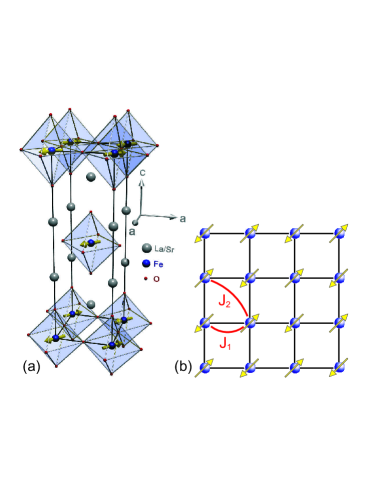
Figure 1: (Color online) (a) Visualization of the crystal and magnetic structure of LaSrFeO₄. (b) Tetragonal basal plane showing only the magnetic Fe ions in order to declare the coupling constants $J_{1}$ and $J_{2}$.

II Experimental

The sample preparation has been carried out similar to reported techniques.Oka and Unoki (1987); Bansal et al. (2003) Powder samples of LaSrFeO₄ have been prepared by mixing La₂O₃, SrCO₃ and Fe₂O₃ in the stoichiometric ratio and sintering at 1200^∘C for 100 h. Diffraction patterns were taken on a Siemens D5000 X-ray powder diffractometer in order to confirm the correct phase formation (space group $I4/mmm$) and the absence of parasitic phases. Furthermore, the lattice constants were deduced at those temperatures used in the neutron study due to the higher precision of the powder method.
Large single crystals of LaSrFeO₄ have been grown by the floating-zone method. Therefore, LaSrFeO₄ powder was pressed into a cylindrical rod of 60 mm length and 8 mm diameter and sintered at 1300^∘C for 20 h. The crystal has been grown in a floating-zone furnace (Crystal Systems Incorporated) equipped with four halogen lamps (1000 W). The feed and seed rods were rotated in opposite directions at about 10 rpm, while the molten zone was vertically moved at a growth speed of 3 mm/h. This procedure has been performed under a pressure of 4 bars in argon atmosphere. Suitable single crystals for X-ray diffraction have been obtained by milling larger pieces in a ball mill for serveral hours. The characterization at the X-ray single crystal diffractometer Bruker Apex D8 validated the successful crystal growth. The magnon dispersion has been investigated at the thermal and cold neutron triple-axis spectrometers 2T and 4F.2 at the Laboratoire Léon Brillouin (LLB) using a large single crystal of 3.33 g weight, whose single crystal state was verified at a Laue diffractometer. For energy transfers above 20 meV inelastic data has been recorded on the 2T spectrometer, which was used with a pyrolytic graphite (PG) monochromator and a PG analyzer. The final neutron energy was fixed at either $E_{f}=34.9$ meV, $E_{f}=14.7$ meV, or $E_{f}=8.04$ meV. The 4F.2 spectrometer was used with a PG double monochromator and PG analyzer. A cooled Be filter was used to suppress higher harmonics. The final neutron energy was fixed at $E_{f}=4.98$ meV.
The nuclear and magnetic structure determination has been carried out at the neutron single-crystal diffractometer 5C2 (LLB) situated at the hot source of the Orphée reactor. For the elastic measurements a smaller single crystal of 39 mg has been used. A wavelength of 0.83 Å  has been employed supplied by the (220) reflection of a Cu monochromator. The Néel temperature was derived at the 3T.1 spectrometer (LLB) using a furnace. Magnetization data was obtained by a commercial superconducting quantum interference device (SQUID) and a vibrating sample magnetometer (VSM). Electric resistivity has been measured by the standard four-contact method.

III Results and discussion

III.1 Macroscopic properties

The magnetization data obtained from the SQUID do not show any additional magnetic phase transitions between 1.8 K and 300 K (Fig. 2). An additional measurement in a VSM with an oven did not reveal any signature of $T_{N}$ in the measured range from 300 K to 800 K. Such a behaviour is characteristic for the layered magnetism in 214 compounds, where the ordering temperature has only been unambiguously determined by neutron diffraction experiments.Senff et al. (2008) The fact that the Fe magnetic moments exhibit two-dimensional correlations well above $T_{N}$ renders it impossible to detect this transition macroscopically. The transition from two-dimensional to three-dimensional magnetic order can however be seen via neutron diffraction. Fig. 3 shows the specific resistivity as a function of temperature. No reliable data could be obtained below 175 K due to the high values of $\rho$. The high-temperature data has been plotted in a $\ln(\sigma)$-$\frac{1}{T}$ plot to which an Arrhenius function ($\ln{\sigma}=\ln{\sigma_{0}}-\frac{E}{2kT}$) has been fitted (shown in inset). From the linear behavior a band gap of $\Delta$=0.525(1) eV can be deduced. At 200 K a kink is visible in the specific resistivity whose origin is not yet clear to us.

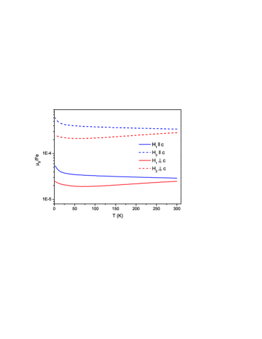
Figure 2: (Color online) Magnetization given in Bohr magnetons per Fe atom as a function of temperature for two different applied magnetic fields parallel and perpendicular to the $c$ axis ($H_{1}$=100 Oe, $H_{2}$=1000 Oe). No hints for a magnetic phase transition can be observed between 1.8 K and 300 K.

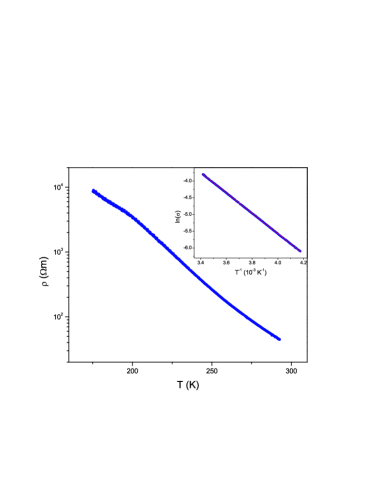
Figure 3: (Color online) Specific resistivity of LaSrFeO₄ as a function of temperature. An Arrhenius fit ($\ln{\sigma}=\ln{\sigma_{0}}-\frac{E}{2kT}$) to the high-temperature data yields a band gap of $\Delta$=0.525(1) eV.

III.2 Nuclear structure

The investigation of the powder samples by X-ray diffraction confirmed the reported crystal structure. All powder diffraction patterns were analyzed using the FullProf program.Rodríguez-Carvajal (1993) Fig. 4 depicts the powder pattern recorded at room temperature. The calculated pattern [(black) solid line] agrees very well with the observed pattern [(red dots)] and no parasitic peaks can be observed. Additional diffraction patterns were recorded at 120 K, 50 K and 10 K. The lattice parameters have been deduced and are listed in Tab. 1.

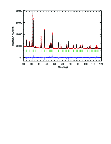
Figure 4: (Color online) X-ray powder diffraction pattern of LaSrFeO₄ taken at room temperature. Raw data are depicted by (red) dots, while the calculated pattern and the difference line are represented by solid (black) and by solid (blue) lines, respectively. (Green) vertical bars indicate the position of Bragg reflections.

For the nuclear structure investigation at the neutron single crystal diffractometer a total number of 739 independent reflections has been collected at each temperature. The integrated intensities were corrected for absorption applying the transmission factor integral $\exp[-\mu(\tau_{in}+\tau_{out})]$ by using subroutines of the Cambridge Crystallographic Subroutine LibraryMatthewman et al. (1982) ($\tau_{in}$ and $\tau_{out}$ represent the path lengths of the beam inside the crystal before and after the diffraction process, $\mu$ is the linear absorption coefficient, which is 0.146 cm^-1 for LaSrFeO₄). The nuclear structure refinement included the $z$ value of the atomic positions of La/Sr and O2, the anisotropic temperature factors of all ions (respecting symmetry restrictions according to Ref. Peterse and Palm, 1966), the occupation of the O1 and O2 site as well as the extinction parameters according to an empiric ShelX-like model.Larson (1970) All refined structural parameters are shown in Tab. 1. The atomic positions show almost no significant dependence on the temperature, while the lattice constants and anisotropic displacement parameters (ADP) expectedly decrease with decreasing temperature. The only exception are the $U_{33}$ parameters, which increase for all species when reducing the temperature from 50 K to 10 K. This results in a much more anisotropic atomic displacement at 10 K with more out-of-plane motion. One may realize that some of the ADPs are stronger than it might be expected from the phononic contributions. It has already been pointed out in earlier studies on La_2-xSr_xCuO₄ (Ref. Braden et al., 2001) and La_1+xSr_1-xMnO₄ (Ref. Senff et al., 2005) that the intrinsic disorder due to the occupation of the same site by La and Sr causes a non-zero force on the oxygen ions at the mean atomic positions derived by diffraction experiments. Due to the La/Sr-O bonds being perpendicular to the Fe-O bonds the disorder will affect the displacement of the O ions mainly perpendicular to the Fe-O bonds, i.e. the $U_{33}$ parameter of O1 and the $U_{11}$ parameter of O2 are most affected. The refinement indeed yields pronounced enhancement of these parameters. From the neutron data an eventual oxygen deficiency might be deduced. Taking into account the refinement with the best agreement factors one can calculate the stoichiometry of the investigated compound to be LaSrFeO_3.92(6) yielding a slight oxygen deficiency.

Table 1: Nuclear structure parameters within the $I4/mmm$ space group at different temperatures. The Wyckoff sites are La/Sr 4$e$ (00$z$), Fe 2$a$ (000), O1 4$c$ (0$\frac{1}{2}$0) and O2 4$e$ (00$z$). The results of the neutron single crystal diffraction experiment were completed by measuring the lattice constants using X-ray powder diffraction. For La/Sr, Fe and O2 $U_{22}$ is constrained by symmetry to $U_{11}$.

	T (K)	10 K	50 K	120 K	RT
	$a$ (Å)	3.8709(1)	3.8713(1)	3.8726(1)	3.8744(1)
	$c$ (Å)	12.6837(4)	12.6848(4)	12.6931(4)	12.7134(3)
La/Sr	$z$	0.3585(1)	0.3589(1)	0.3589(1)	0.3587(1)
	$U_{11}$ (Å2)	0.0032(6)	0.0056(5)	0.0067(5)	0.0107(5)
	$U_{33}$ (Å2)	0.007(1)	0.0045(4)	0.0044(4)	0.0089(5)
Fe	$U_{11}$ (Å2)	0.0017(7)	0.0036(4)	0.0047(4)	0.0069(6)
	$U_{33}$ (Å2)	0.013(1)	0.0099(5)	0.0121(5)	0.0186(7)
O1	occ (%)	99(2)	102(2)	102(2)	99(2)
	$U_{11}$ (Å2)	0.0050(9)	0.009(1)	0.007(2)	0.011(1)
	$U_{22}$ (Å2)	0.0034(9)	0.003(2)	0.006(2)	0.0074(9)
	$U_{33}$ (Å2)	0.012(1)	0.0085(4)	0.0097(5)	0.0175(9)
O2	occ (%)	97(2)	97(2)	97(2)	96(2)
	$z$	0.1694(2)	0.1686(1)	0.1689(1)	0.1692(2)
	$U_{11}$ (Å2)	0.0160(9)	0.0160(4)	0.0179(7)	0.0230(8)
	$U_{33}$ (Å2)	0.011(1)	0.0079(7)	0.0077(6)	0.0124(7)
	$R_{F}$ (%)	2.65	2.84	3.17	2.78
	$\chi^{2}$	0.33	2.35	2.05	4.60

III.3 Magnetic structure

We found strong half-indexed magnetic Bragg peaks confirming the known propagation vector $\mathbf{q}_{1}=(\frac{1}{2}\frac{1}{2}0)$. The intensity of the magnetic $(\frac{1}{2}\frac{1}{2}0)$ reflection was measured as a function of temperature and is shown in Fig. 5. A power-law fit to the integrated intensity data yields a Néel temperature of 366(2) K and a critical exponent $\beta$=0.15(5) (upper right inset). However, an exact determination of $T_{N}$ is hardly possible as significant intensity due to strong quasielastic scattering can be observed well above the transition temperature e.g. at 400 K or 460 K. By scanning across the forbidden (010) reflection an eventual $\lambda/2$ contamination can be ruled out (upper left inset).

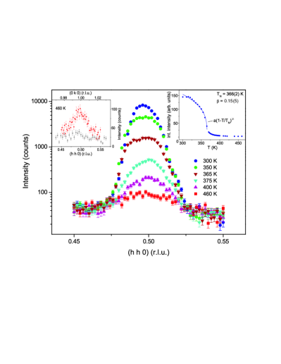
Figure 5: (Color online) Longitudinal $\mathbf{q}$-scan across the magnetic $(\frac{1}{2}\frac{1}{2}0)$ reflection (the intensity is plotted on a log-scale). The inset at the upper right shows the integrated intensity as a function of temperature. A power-law fit yields a $T_{N}$ of 366(2) K. The inset at the upper left depicts the same longitudinal $\mathbf{q}$-scan at 460 K [(red) filled squares] together with a longitudinal $\mathbf{q}$-scan across the forbidden (010) reflection [(black) open circles] documenting that no $\lambda/2$ contamination is present.

As two additional magnetic phase transitions might be expected at 90 K and 30 K (Ref. Jung et al., 2005) the magnetic structures have been investigated at 120 K, 50 K and 10 K. For the magnetic structure refinement a total number of 185 independent reflections has been recorded at each temperature point, where the integrated intensities have been corrected for absorption. Representation analysis has been used to derive symmetry adapted spin configurations which were then refined to the respective data. Three irreducible representations are compatible with the space group $I4/mmm$ yielding collinear spin configurations with the moments parallel to the $c$ axis, parallel to $\mathbf{q}$ or perpendicular to $\mathbf{q}$, the last two being of orthorhombic symmetry. Due to the fact that $\mathbf{q}_{2}=(-\frac{1}{2}\frac{1}{2}0)$ is a possible propagation vector as well each of the irreducible representations with the basis vectors in the a-b plane will exhibit two magnetic orientations. The domains are connected to each other by the symmetry operator (y,-x,z) which has been lost during the transition into the magnetically ordered state. The relevant spin configurations used in previous analysesSoubeyroux et al. (1980); Jung et al. (2005) are shown in Fig. 6.

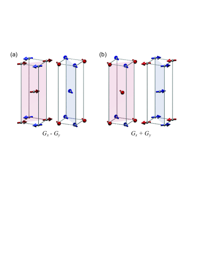
Figure 6: (Color online) Magnetic G-type ordering (according to standard Wollan-Koehler notationWollan and Koehler (1955)) in LaSrFeO₄ only showing the magnetic Fe ions and their spins for the two $\mathbf{q}$-domains. (a) shows the irreducible representation labelled $G_{x}-G_{y}$ which has the magnetic moments perpendicular to $\mathbf{q}_{1}$ (left) and $\mathbf{q}_{2}$ (right). (b) shows the irreducible representation labelled $G_{x}+G_{y}$ with the magnetic moments parallel to $\mathbf{q}_{1}$ (left) and $\mathbf{q}_{2}$ (right).

The data could well be described by the model $G_{x}-G_{y}$, where the size and the direction (angle $\phi$ between the moment and the $a$ axis) of the magnetic moments in the basal plane as well as the percental distribution between the two magnetic domains were refined. The results are listed in Tab. 2 for all investigated temperatures. In Refs. Soubeyroux et al., 1980 and Jung et al., 2005 the authors claim that their sample exhibits an inhomogeneous distribution of the two collinear representations $G_{x}-G_{y}$ and $G_{x}+G_{y}$ accounting for 92% and 8% of the sample volume. Furthermore, the intensity jumps of characteristic magnetic Bragg reflections at the transition temperatures 30 K and 90 K were attributed to a change in the relative distribution of the representations. We have followed the integrated intensity of characteristic magnetic Bragg reflections as a function of temperature across the two lower magnetic phase transitions and could not observe any significant jumps (Fig. 7). Although the statistics seem to be limited in comparison to the size of the jumps at least for the (0.5 0.5 1) reflection, one can state that the scattering from both domains does not exhibit contrary behavior in dependence of temperature ruling out a redistribution of domain population. We have applied the proposed inhomogeneous distribution of two representations to our data, however, no significant contribution of $G_{x}+G_{y}$ is present (see Tab. 2).

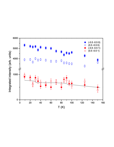
Figure 7: (Color online) Integrated intensity of characteristic magnetic Bragg reflections probing either domain $\mathbf{q}_{1}$ (positive $h$ values) or domain $\mathbf{q}_{2}$ (negative $h$ values) as a function of temperature. The solid line represents the size of the jumps reported in Ref. Jung et al., 2005.

Table 2: Results of the magnetic structure refinement.

T (K)	10 K	50 K	120 K
$m_{Fe}$ ($\mu$${}_{\mbox{B}}$)	4.96(1)	5.38(1)	5.09(1)
$\phi$ (deg)	44.0(8)	44.9(8)	46.7(8)
domain $\mathbf{q}_{1}$ (%)	46.5(4)	47.3(4)	47.7(5)
domain $\mathbf{q}_{2}$ (%)	53.5(4)	57.7(4)	52.3(5)
$G_{x}-G_{y}$ (%)	98(2)	97(2)	98(2)
$G_{x}+G_{y}$ (%)	2(2)	3(2)	2(2)
$R_{F}$ (%)	5.14	4.43	4.76
$\chi^{2}$	1.78	1.75	1.95

III.4 Magnon dispersion

The magnon dispersion has been investigated at 10 K along the two main-symmetry directions [0 $\xi$ 0] and $[\xi$ -$\xi$ 0]. Depending on the orientation of the resolution ellipsoid with respect to the dispersion branch constant-$\mathbf{Q}$ or constant-E scans have been performed. The excitation signals have been fitted with two symmetrical Gauss functions (constant-$\mathbf{Q}$ scans) or an asymmetric double-sigmoid (constant-E scans) in order to account for the strong asymmetry at high energy transfers. An asymmetry has been applied to the symmetric Gauss functions for the constant-$\mathbf{Q}$ scans at higher energy transfer. Exemplary scans are shown in Fig. 8 documenting the data analysis.

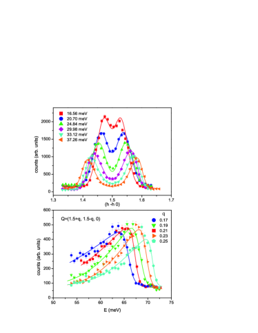
Figure 8: (Color online) Exemplary scans showing how the values of $S(q,\omega)$ have been obtained. Constant-E scans have been fitted with two symmetric Gauss functions (upper plot), while constant-$\mathbf{Q}$ scans have been fitted with asymmetric double sigmoids (lower plot).

According to the magnetic structure, where the magnetic moments are lying in the tetragonal basal plane, two gapped excitations have to be expected. The lower one should be connected to the amount of energy needed to turn a spin out of its ordered position within the basal plane whereas the higher one results from turning a spin out of the plane. Constant-$\mathbf{Q}$ scans have been performed at different Brillouin zone centers in order to derive the size of the respective spin gaps. In Fig. 9(a)-(c) a clear signal can be observed at 5.26(2) meV [the value has been obtained from an asymmetric double-sigmoid fit to the scan at $\mathbf{Q}$=(1.5 0.5 0)], which we identify as the higher-lying out-of-plane gap $\Delta_{out}$. In Fig. 9(c) an additional signal appears at 8.5(2) meV which, however, is not present in the lower zone center scans and therefore rather phononic than magnetic. It can be seen especially in Fig. 9(a) and (b) that the scattered intensity is not reduced to the background below $\Delta_{out}$. Bearing in mind the energy resolution of 0.23 meV as obtained from the FWHM of the elastic line we conclude that the scattered intensity at low energy originates from the in-plane fluctuation of the magnetic moments. Due to the finite size of the resolution ellipsoid and its inclination in $S(q,\omega)$ space signals from steep dispersion branches become very broad as can be seen in Fig. 9(b), where considerable scattered intensity is observed well above 10 meV. For this reason we expect the in-plane fluctuations to be gapless.

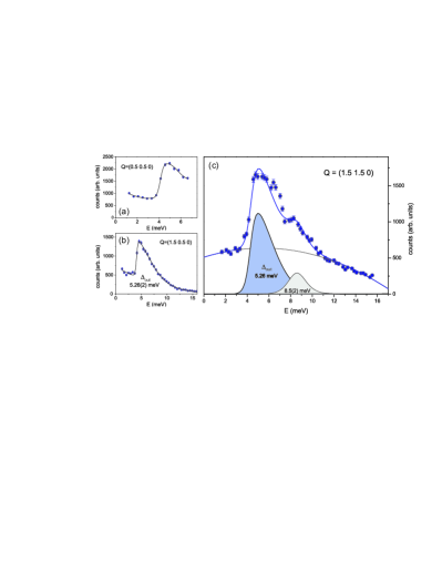
Figure 9: (Color online) Constant-$\mathbf{Q}$ scans at the magnetic zone centers (a) (0.5 0.5 0), (b) (1.5 0.5 0) and (c) (1.5 1.5 0). The excitations have been fitted by asymmetric double sigmoid functions on a polynomial background. The out-of-plane anisotropy gap amounts to 5.26(2) meV as obtained by a fit to the data in panel (b). In panel (c) the signal at 8.5(2) meV is presumably phononic as the same scan at lower $\mathbf{Q}$ values, see panel (b), is featureless at this energy. $\Delta_{out}$ has been held constant in the fit to the data shown in panel (c). The fit curve in panel (a) serves as a guide to the eye. The considerable scattered intensity below $\Delta_{out}$ is a hint for the lower-lying in-plane excitation.

Within linear spin wave theory we used a Hamiltonian of a Heisenberg antiferromagnet with isotropic nearest ($J_{1}$) and next-nearest neighbor ($J_{2}$) interactions [see Fig. 1(b)] as well as an effective magnetic anisotropy field $H_{A}$ along the $z$ axisMarshall and Lovesey (1971)

$$H =\sum_{\mathbf{m,r}}J_{1}(\mathbf{r})\mathbf{S_{m}}\cdot\mathbf{S_{m+r}}+\sum_{\mathbf{m,R}}J_{2}(\mathbf{R})\mathbf{S_{m}}\cdot\mathbf{S_{m+R}}$$

$$+\sum_{\mathbf{n,R}}J_{2}(\mathbf{R})\mathbf{S_{n}}\cdot\mathbf{S_{n+R}}+g\mu_{B}H_{A}\left(\sum_{m}S^{z}_{\mathbf{m}}-\sum_{n}S^{z}_{\mathbf{n}}\right).$$

Here the magnetic lattice has been divided into two identical sublattices $m$ and $n$ where each of them only contains parallel spins. $\mathbf{r}$ is a connection vector between magnetic moments of the interpenetrating antiferromagnetically coupled ($J_{1}$) sublattices with respective positions $\mathbf{m}$ and $\mathbf{n}$, while $\mathbf{R}$ denotes a connection vector between two ferromagnetically coupled magnetic moments of the same sublattice ($J_{2}$). Each spin pair contributes only once to the sum. The diagonalization of the HamiltonianMarshall and Lovesey (1971) leads to the dispersion relation for this particular crystal structure:

$$\hbar\omega_{q} =\{[4SJ_{1}-4SJ_{2}[1-\cos{(2\pi q_{x})}\cos{(2\pi q_{y})}]$$

$$+g\mu_{B}H_{A}]^{2}-(2SJ_{1})^{2}[\cos{(2\pi q_{x})}+\cos{(2\pi q_{y})}]^{2}\}^{\frac{1}{2}}.$$ (2)

We have fitted the dispersion relation simultaneously to spin waves propagating along [0 $\xi$ 0] and [$\xi$ -$\xi$ 0]. With an expected $S=2.5$ we obtain $J_{1}=7.4(1)$ meV, $J_{2}=0.4(1)$ meV and $\mu_{B}H_{A,out}=0.097(2)$ T (note that a factor 2 has been added to the $J$ values for a correct comparison with Refs. Larochelle et al., 2005; Nakajima et al., 1993; Babkevich et al., 2010; Coldea et al., 2001 due to a different definition of the sums in the Hamiltonian). The agreement with the experimental data is fairly well, the dispersion curve is depicted as a black solid line in Fig. 10. Setting $J_{2}$=0 yields $J_{1}$=6.99(1) and $\mu_{B}H_{A,out}=0.102(2)$ T and the agreement is comparable [(red) dashed line in Fig. 10]. While along [$\xi$ -$\xi$ 0] the dispersion is practically unchanged, it goes to higher energy values at the zone-boundary for the propagation along [0 $\xi$ 0], however, staying within the error bars of the data points. The fact that $J_{2}$ is not essentially needed to describe the dispersion makes it possible to apply the spin-wave dispersion reported in Ref. Thurlings et al., 1982, which has been derived for the isostructural K₂FeF₄ structure. This spin Hamiltonian for Fe²⁺ in a tetragonally distorted cubic crystal field only contains a nearest-neighbour exchange parameter, but considers two non-degenerate spin-wave dispersion branches, which - in a semiclassical picture - correspond to elliptical precessions of the spins with the long axis of the ellipse either in or perpendicular to the layer.Thurlings et al. (1982) The spin-wave dispersion is given in Eq. 3 for the larger orthorhombic cell

$$\hbar\omega_{q} =4S|J|[(1+A)^{2}$$

$$-(\cos{[\pi(q_{x}+q_{y})]}\cos{[\pi(q_{x}-q_{y})]}\pm B)^{2}]^{\frac{1}{2}}$$ (3)

with $A=(D-3E)/(4|J|)$ and $B=(D+E)/(4|J|)$. $D$ is a parameter describing the uniaxial anisotropy and $E$ adds an in-layer anisotropy. Fitting Eq. 3 with $E=0$ to both data sets simultaneously yields the values $J$=7.00(1) meV and $D$=0.0409(6) meV. The two non-degenerate branches are depicted as white solid lines in Fig. 10. The upper branch coincides exactly with the formalism in Eq. 2 (only nearest-neighbour interaction) yielding the same coupling constant within the error bars. The lower branch is gapless as predicted by $E$=0 and the reason for the non-zero intensity below $\Delta_{out}$ in Fig. 9.

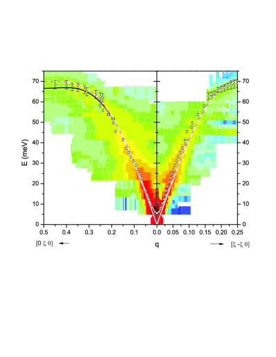
Figure 10: (Color online) Two-dimensional reconstruction of $S(q,\omega)$ along the two symmetry directions [0 $\xi$ 0] and [$\xi-\xi 0$] from all constant-$\mathbf{Q}$ and constant-E scans as exemplarily shown in Fig. 8. Dots mark the peak center as obtained from the fits to the raw data. The straight white line is a fit of the dispersion relation (Eq. 2) to both data sets simultaneously.

An examination of the energy gaps as a function of temperature yielded no differences between 10 K and 100 K.

IV Conclusion

We have conducted a comprehensive study on the single-layered perovskite LaSrFeO₄. Our X-ray powder and single crystal diffraction as well as Laue diffraction yield high sample quality, while our magnetization data differ from previously published work. Detailed investigation of the nuclear structure by neutron diffraction on a single crystal reveals that the intrinsic disorder on the La/Sr site leads to a stronger atomic displacement of the O1 and O2 ions in LaSrFeO₄ in analogy to La_1+xSr_1-xCuO₄ (Ref. Braden et al., 2001) and La_1+xSr_1-xMnO₄ (Ref. Senff et al., 2005). The main results of our study concern the magnetic structure and the magnon dispersion of this compound, which we analyzed by neutron diffraction and inelastic neutron scattering. We have addressed the open question concerning the magnetic phase transitions at 90 K and 30 K. Our SQUID data did not yield any hint for additional magnetic phase transitions and based on our neutron diffraction data we are able to say that no spin reorientation or domain/representation redistribution is present. Possible discrepancies between the data of different studies might be the exact amount of oxygen as these systems are known to exhibit oxygen deficiency. From the nuclear structure refinement we can deduce the oxygen deficiency to be $y=0.08(6)$ in LaSrFeO_4-y. The large number of measured reflections allows an analysis of the magnetic form factor. Therefore, the observed magnetic structure factors were divided by the exponential part of the calculated magnetic structure factor and the ordered moment. The resulting observed magnetic form factor has been derived for (hk0) and (hkl) reflections in order to gain information about the in-plane and out-of-plane atomic magnetization density distribution in LaSrFeO₄. In Fig. 11 the observed magnetic form factors for both kinds of magnetic reflections are depicted showing a tendency towards weaker decrease with increasing $\sin(\theta)/\lambda$ in comparison to the tabulated analytical approximation of the Fe³⁺ magnetic form factor, which would imply a more localized atomic magnetization density distribution. However, due to the limited number of (hk0) reflections and the size of the error bars no significant anisotropy can be deduced.

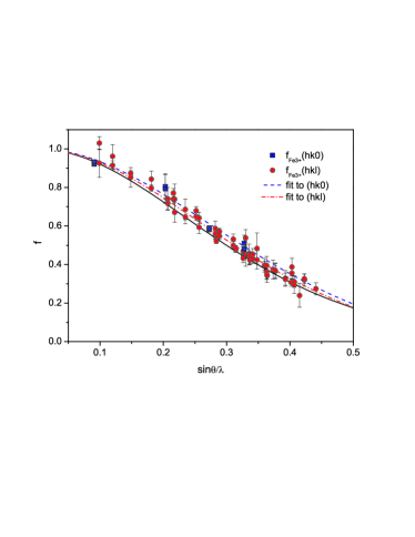
Figure 11: (Color online) Observed magnetic Fe form factor for (hk0) [(blue) squares] and (hkl) [(red) dots] magnetic reflections. The (black) solid line depicts the tabulated analytical approximation of the Fe³⁺ form fator. The data have been fitted by varying the tabulated values while requiring f(0)=1 [(red) dash-dotted line is the fit to the (hkl) data, (blue) dashed line is the fit to the (hk0) data].

In addition, we have analyzed the magnon dispersion along the two symmetry directions [0 $\xi$ 0] and [$\xi$ -$\xi$ 0]. Within linear spin wave theory we can describe both branches with the nearest neighbor and next-nearest neighbor interaction $J_{1}=7.4(1)$ meV and $J_{2}=0.4(1)$ meV, respectively ($S=2.5$). These values are more than a factor 2 larger than those in the isostructural undoped LaSrMnO₄ with $S=2$ (Ref. Larochelle et al., 2005), which can be attributed to the fact that $e_{g}$-$e_{g}$ superexchange contributes only little for the case of the Mn orbital arrangement in LaSrMnO₄. Our data indicate two non-degenerate spin-wave dispersion branches. A clear signal at 5.26(2) meV was identified as the out-of-plane anisotropy gap $\Delta_{out}$. The non-zero scattered intensity at lower energy transfers is explained by the lower-lying anisotropy gap, which was then analyzed by using the formalism described in Ref. Thurlings et al., 1982. With a nearest-neighbour interaction $J$=7.00(1) meV and the anisotropy parameters $D$=0.0409(6) and $E$=0 a good agreement between the upper dispersion branch and the experimental data has been achieved, while the lower branch goes down to zero-energy transfer at the magnetic zone center. The spin wave dispersion in La₂NiO₄ is also well described by a nearest neighbor interaction only,Nakajima et al. (1993) but with $J=31$ meV it is a factor of 4 stronger than in LaSrFeO₄ indicating higher hybridization in La₂NiO₄. Although a more involved Hamiltonian has been used for the description of the spin dynamics in La₂CoO₄ (with high-spin $S$=$\frac{3}{2}$ Co²⁺) including three coupling constants and corrections for spin-orbit coupling, ligand and exchange fields,Babkevich et al. (2010) the resulting coupling constants are of the same order as the ones presented here. Furthermore, the out-of-plane gap and the bandwidth are quite comparable. In order to compare the single-ion anisotropy of the involved species within one model we have used Eq. 2 together with the $J$ values given in Refs. Larochelle et al., 2005; Nakajima et al., 1993; Babkevich et al., 2010; Coldea et al., 2001 (up to next-nearest neighbour exchange) to calculate the anisotropy parameter $\mu_{B}H_{A,out}$. The approximate values of the dispersion at the zone center and zone boundary were taken from plots within Refs. Larochelle et al., 2005; Nakajima et al., 1993; Babkevich et al., 2010; Coldea et al., 2001. The comparison of $J$ and $H_{A,out}$ for the different compounds is shown in Tab. 3.

Table 3: Comparison of the exchange coupling and anisotropy parameters of LaSrFeO₄ with other 214 compounds [LaSrMnO₄ (Ref. Larochelle et al., 2005), La₂CoO₄ (Ref. Babkevich et al., 2010), La₂NiO₄ (Ref. Nakajima et al., 1993), La₂CuO₄ (Ref. Coldea et al., 2001)].

	Mn	Fe	Co	Ni	Cu
$S$	2	2.5	1.5	1	0.5
$J_{1}$ (meV)	3.4(3)	7.4(1)	9.69(2)	31	104(4)
$J_{2}$ (meV)	0.4(1)	0.4(1)	0.43(1)	0	-18(3)
$\mu_{B}H_{A,out}$ (T)	0.65	0.097(2)	0.67	0.52	0

One can see that the single-ion anisotropy of the Fe³⁺ in LaSrFeO₄ is significantly smaller than in the other 214 compounds (except for La₂CuO₄), which is expected due to the close to zero orbital moment and therefore very weak spin-orbit coupling.