A block MINRES algorithm based on the band Lanczos method

Abstract

We develop a block minimum residual (MINRES) algorithm for symmetric indefinite matrices. This version is built upon the band Lanczos method that generates one basis vector of the block Krylov subspace per iteration rather than a whole block as in the block Lanczos process. However, we modify the method such that the most expensive operations are still performed in a block fashion. The benefit of using the band Lanczos method is that one can detect breakdowns from scalar values arising in the computation, allowing for a handling of breakdown which is straightforward to implement.

We derive a progressive formulation of the MINRES method based on the band Lanczos process and give some implementation details. Specifically, a simple reordering of the steps allows us to perform many of the operations at the block level in order to take advantage of communication efficiencies offered by the block Lanczos process. This is an important concern in the context of next-generation super computing applications.

We also present a technique allowing us to maintain the block size by replacing dependent Lanczos vectors with pregenerated random vectors whose orthogonality against all Lanczos vectors is maintained. Numerical results illustrate the performance on some sample problems. We present experiments that show how the relationship between right-hand sides can effect the performance of the method.

1 Introduction

We wish to efficiently solve

$$\mathbf{A}\mathbf{X}=\mathbf{B}$$ (1)

where $\mathbf{A}\in\mathbb{R}^{n\times n}$ is a symmetric, indefinite matrix, and $\mathbf{B}\in\mathbb{R}^{n\times p}$ with $p$ right-hand sides. If $p=1$, Krylov subspace methods such as the minimum residual MINRES method of Paige and Saunders [17] have been shown to be effective. For the case $p>1$, block Krylov subspace methods have been proposed; see, e.g., [8, 15, 16, 27]. In general, a block Krylov subspace method functions in the same manner as a Krylov subspace method, but at each iteration the operator is applied to a block of vectors rather than just one. These methods generate $p$ new orthonormal basis vectors per iteration. Many scalar operations become operations involving small, dense matrices. With these methods one can simultaneously solve the linear system for $p$ right-hand sides or solve a system with one right-hand side but over a block Krylov subspace. Though block methods increase the per iteration costs (as measured by floating-point operation counts), they can be more efficient from the standpoint metrics related to movement of data within the computer.

Our goals in this work are to develop a method which

1. solves (1) over a block Krylov subspace for any $p\geq 1$,

2. is designed to take advantage of the communication efficiencies of block operations (when possible) but with greater ease of implementation,

3. is able to detect breakdowns through quantities arising in the computation,

4. and maintains the block size when a breakdown occurs.

Therefore, we seek a Lanczos-type method to generate the block Krylov basis one vector per iteration, which is amenable to reordering of the steps to perform as many computations in blocks (e.g., sparse block operations or dense BLAS-3 operations) as possible. Furthermore, upon detection of a breakdown we prefer a strategy which maintains the block size by replacing the dependent Lanczos vector.

To this end we introduce a version of the MINRES algorithm for block Krylov subspaces which satisfies our requirements. This algorithm is built upon the band Lanczos process of Ruhe [20], which generates a basis for the block Krylov subspace one vector at a time rather than in a block fashion. Our algorithm can be considered a simplification of the algorithm presented in [1], which extends Ruhe’s band Lanczos to generalize the nonsymmetric Lanczos process to the block setting in the case that $\mathbf{A}$ is symmetric. However, we make modifications to execute some operations in a block fashion.

We present the theoretical derivation needed to develop a minimum residual method based on the band Lanczos procedure. We also discuss the simple modifications needed to execute some operations in a block fashion as well as some practical implementation details, to simplify the writing of the code. To our knowledge this is the first paper to provide implementation details of a block minimum residual algorithm for symmetric matrices.

In the next section, we introduce notation and give a brief review of Krylov subspace methods (both non-block and block). In Section 3, we derive a version of the block minimum residual method built upon the band Lanczos method. In Section 4, we derive the progressive formulation of this method in detail, which is built to take advantage of the potential memory savings afforded by the method. In Section 5, we present modifications to our implementation which accommodate the occurrence of exact or inexact dependence of a candidate block Krylov subspace basis vector. In Subsection 5.1, we develop a technique to maintain the block size when breakdown occurs. In Section 6, we discuss convergence properties of block methods. In Section 7, special attention is given to how certain data is stored to keep the scheme as simple as possible. In Section 8, we present numerical results.

2 Preliminaries

For the matrix $\mathbf{A}$ and starting vector $\mathbf{r}_{0}$ recall that we generate an orthonormal basis for the Krylov subspace

$${\mathcal{K}}_{j}(\mathbf{A},\mathbf{r}_{0})=\text{span}\left\{\mathbf{r}_{0},\mathbf{A}\mathbf{r}_{0},\ldots,\mathbf{A}^{j-1}\mathbf{r}_{0}\right\}$$

with the Arnoldi process. Let $\mathbf{V}_{j}\in\mathbb{R}^{n\times j}$ be the matrix with orthonormal columns consisting of this basis. Then we have the Arnoldi relation

$$\mathbf{A}\mathbf{V}_{j}=\mathbf{V}_{j+1}\overline{\mathbf{H}}_{j}$$ (2)

with $\overline{\mathbf{H}}_{j}\in\mathbb{R}^{(j+1)\times j}$; see, e.g., [21, Section 6.3] and [25]. In the case $p=1$, we can solve (1) with a Krylov subspace iterative method. Suppose $\mathbf{x}_{0}$ is an initial approximation, and $\mathbf{r}_{0}=\mathbf{B}-\mathbf{A}\mathbf{x}_{0}$ is the initial residual. At iteration $j$, we can compute the minimum residual correction $\mathbf{t}_{j}\in{\mathcal{K}}_{j}(\mathbf{A},\mathbf{r}_{0})$ satisfying $\mathbf{t}_{j}=\underset{\mathbf{t}\in{\mathcal{K}}_{j}(\mathbf{A},\mathbf{r}_{0})}{\text{{\rm argmin}}}\left\|\mathbf{B}-\mathbf{A}(\mathbf{x}_{0}+\mathbf{t})\right\|$ by solving the equivalent small least squares problem $\mathbf{y}_{j}=\underset{\mathbf{y}\in\mathbb{R}^{j+1}}{\text{{\rm argmin}}}\left\|\left\|\mathbf{r}_{0}\right\|\mathbf{e}_{1}^{(j+1)}-\overline{\mathbf{H}}_{j}\mathbf{y}\right\|$ and setting $\mathbf{t}_{j}=\mathbf{V}_{j}\mathbf{y}_{j}$. Implementations of minimum residual methods include GMRES [22] in the nonsymmetric case and MINRES [17] in the symmetric case.

Much has been written about the solution of linear systems with multiple right-hand sides. Extending the framework of a Krylov method to the block right-hand side setting involves generalizing the machinery to deal with block vectors; see, e.g., [21, Page 208].

Let $\mathbf{V}_{1}\in\mathbb{R}^{n\times p}$ be a matrix with orthonormal columns. At step $j$, the block Arnoldi process generates an orthonormal basis for a block Krylov subspace

$$\mathbb{K}_{j}(\mathbf{A},\mathbf{V}_{1})={\mathcal{K}}_{j}(\mathbf{A},\mathbf{v}_{1}^{(1)})+{\mathcal{K}}_{j}(\mathbf{A},\mathbf{v}_{1}^{(2)})+\cdots+{\mathcal{K}}_{j}(\mathbf{A},\mathbf{v}_{1}^{(p)}).$$

where $\mathbf{V}_{1}=\left[\begin{matrix}\mathbf{v}_{1}^{(1)},&\mathbf{v}_{1}^{(2)},&\ldots,&\mathbf{v}_{1}^{(p)}\end{matrix}\right]$. In this setting sparse matrices act on a block of vectors per iteration. For this discussion, we assume for now that $\dim\mathbb{K}_{m}(\mathbf{A},\mathbf{V}_{1})=mp$, i.e., no linear dependent block Arnoldi vectors are generated. We will return to the case of dependence later.

A strength of generalizing the Arnoldi process (or Lanczos) is that the block level operations (e.g., BLAS-3 operations for dense matrices and block operations for sparse matrices) have been shown to be quite efficient, when measured in metrics relevant in a high performance computing environment, i.e., amount of data moved through memory, frequency of cache missing, and the number of floating point operations performed on a unit of data while it is in cache. These considerations have led to the broader goal to design communication avoiding Krylov subspace methods; see, e.g., [13]. In next-generation supercomputing machines the movement of data within the machine (e.g., from main memory onto the cache) increasingly will represent the dominant computational cost, and algorithms should be judged according to an appropriate data movement metric [5]. When judged according to such metrics the per iteration data movement costs of a block method are only marginally more expensive than their single vector counterparts (both dense, BLAS-3 operations and sparse block operations). Therefore, we minimize the residual over a larger constraint space without a concomitant increase in computational costs (related to the movement of data). For further work on this topic, see, e.g., [3, 18].

One can also generate the block Krylov subspace one vector at a time using the band Lanczos process proposed by Ruhe [20]. At each iteration one matrix-single-vector product is performed as opposed to a matrix-block-vector product in a block-level method. It proceeds in a similar fashion to the single-vector Arnoldi process but starts with $p$ vectors against which the new vector must be orthogonalized instead of one. We derive our algorithm from this process but with certain operations performed in a block fashion. We must adopt a notation which is compatible with the single vector per iteration nature of the band Lanczos process. Thus the initial block of normalized vectors called $\mathbf{V}_{1}$ before is renamed $\mathbf{U}_{p}=\left[\begin{matrix}\mathbf{u}_{1},\ldots,\mathbf{u}_{p}\end{matrix}\right]$, denoting that we start with the first $p$ orthonormal vectors.

Beginning with no symmetry assumption on $\mathbf{A}$, the band Arnoldi process (see, e.g., [7, 8]) performs the same orthogonalization as the block method, only one vector at a time. We denote the matrix with the first $j$ band Arnoldi vectors as columns $\mathbf{U}_{j}\in\mathbb{R}^{n\times j}$ where for $j<p$, $\mathbf{U}_{j}$ has only the first $j$ starting vectors as columns.

This algorithm allows one to detect a breakdown from the scalar quantities generated by the band Lanczos process. By reordering the computations the band Lanczos algorithm can be formulated with many of the same block level operations as the block Lanczos algorithm, e.g., the operator is applied to a block of vectors every $p$ iterations while maintaining the ease with which we detect breakdown in the band Lanczos algorithm.

To describe the Arnoldi relation in this setting, we must take care as the iteration number $j$ does not match the dimension of the block Krylov subspace. At iteration $j$, we generate the $(j+p)$th band Arnoldi vector. At this iteration we have the band Arnoldi relation

$$\mathbf{A}\mathbf{U}_{j}=\mathbf{U}_{j+p}\overline{\mathbf{H}}_{j}.$$ (3)

The banded Hessenberg matrix $\overline{\mathbf{H}}_{j}\in\mathbb{R}^{(j+p)\times j}$ has $p$ lower subdiagonal entries per column and has the structure

$$\overline{\mathbf{H}}_{j}=\left[\begin{matrix}\mathbf{H}_{j}\\ \mathbf{H}_{p\times j}\end{matrix}\right],$$

where $\mathbf{H}_{j}$ is a square $j\times j$ matrix satisfying the identity

$$\mathbf{H}_{j}=\mathbf{U}_{j}^{\ast}\mathbf{A}\mathbf{U}_{j}.$$ (4)

Observe that $\mathbf{H}_{p\times j}$ only has nonzero entries in the last $p$ columns with structure $\mathbf{H}_{p\times j}=\left[\begin{matrix}\mathbf{0}_{p\times(j-p)}&\mathbf{C}_{j}\end{matrix}\right]$ where $\mathbf{C}_{j}\in\mathbb{R}^{p\times p}$ is upper triangular. At iteration $j$ the dimension of the subspace built is $j+p$.

To unambiguously describe the subspace at each iteration, we identify it with the pair $(k,m)$ determined uniquely by $j=(k-1)p+m$ with $0\leq m<p$. As shown in (5), this pair is used to describe the block Krylov subspace built by the band Lanczos process. The subspace that has been generated at iteration $j$ is the sum of Krylov subspaces generated by each column of $\mathbf{U}_{p}$, i.e.,

$$\mathbb{K}_{k,m}(\mathbf{A},\mathbf{U}_{p})=\underbrace{\sum_{\ell=1}^{m}{\mathcal{K}}_{k+1}(\mathbf{A},\mathbf{u}_{\ell})}_{\varnothing\mbox{\ when\ }m=0}+\sum_{\ell=m+1}^{p}{\mathcal{K}}_{k}(\mathbf{A},\mathbf{u}_{\ell})={\mathcal{R}}\left(\mathbf{U}_{j}\right).$$ (5)

Initially we have the identity, $\mathbb{K}_{1}(\mathbf{A},\mathbf{U}_{p})=\mathbb{K}_{1,0}(\mathbf{A},\mathbf{U}_{p})$. After $p$ iterations we have the following sequence of nested subspaces,

$$\mathbb{K}_{1,1}(\mathbf{A},\mathbf{U}_{p})\subseteq\mathbb{K}_{1,2}(\mathbf{A},\mathbf{U}_{p})\subseteq\cdots\subseteq\mathbb{K}_{1,p}(\mathbf{A},\mathbf{U}_{p}).$$

We observe that, in fact, $\mathbb{K}_{1,p}(\mathbf{A},\mathbf{U}_{p})=\mathbb{K}_{2,0}(\mathbf{A},\mathbf{U}_{p})$, since $m<p$ must hold. The Krylov subspaces in the sum (5) for the first $m$ right-hand sides $\left\{\mathbf{u}_{1},\cdots,\mathbf{u}_{m}\right\}$ are of dimension $k+1$ and the remaining are of dimension $k$. For $j=(K-1)p$, a multiple of the block size, the band Lanczos process has produced an orthonormal basis spanning the $K$th block Krylov subspace generated by $\mathbf{A}$ and $\mathbf{U}_{p}$, i.e.,

$$\mathbb{K}_{K}(\mathbf{A},\mathbf{U}_{p})=\mathbb{K}_{K,0}(\mathbf{A},\mathbf{U}_{p}).$$ (6)

At each iteration one of the subspaces in the sum (5) increases by one dimension.

Similar to the symmetric Lanczos relation in the case of a single-vector Krylov method, observe that if $\mathbf{A}$ is symmetric the relation (4) implies that ${\mathbf{H}}_{j}$ is also symmetric. Due to the banded Hessenberg structure of ${\mathbf{H}}_{j}$, we see that $\overline{\mathbf{H}}_{j}$ is a banded matrix with $p$ superdiagonal entries and $p$ subdiagonal entries per column. This structure implies that the orthogonalization process requires only the most recent $2p$ basis vectors in order to compute $\mathbf{u}_{j+p}$. We have the $2p+1$ term recurrence relation

$$\mathbf{A}\mathbf{u}_{j}=\sum_{\ell=\min\left\{1,j-p\right\}}^{j+p}h_{\ell,j}\mathbf{u}_{\ell}.$$ (7)

Due to symmetry we do not need to compute $h_{\ell,j}$ where $\ell<j$ since it was computed previously as ${h_{j,\ell}}$. This yields Algorithm 2.1, Ruhe’s band Lanczos method.

1

Input : $\mathbf{A}\in\mathbb{R}^{n\times n}$ symmetric, $\mathbf{U}_{p}\in\mathbb{R}^{n\times p}$, $\mathbf{U}_{p}^{\ast}\mathbf{U}_{p}=\mathbf{I}_{p}$

Output : $\mathbf{U}_{j+p}\in\mathbb{R}^{n\times(j+p)}$, $\mathbf{U}_{j+p}^{\ast}\mathbf{U}_{j+p}=\mathbf{I}_{j+p}$ and $\overline{\mathbf{H}}_{j}\in\mathbb{R}^{(j+p)\times m}$, $\overline{\mathbf{H}}_{j}$ is symmetric with $p$ lower subdiagonal entries

2

3for $\ell=1,2,\ldots,j$ do

4       Compute $\mathbf{w}:=\mathbf{A}\mathbf{u}_{\ell}$

5       for $i=\max\left\{1,p-\ell\right\},\ldots,p+\ell-1$ do

6             $h_{i,\ell}:=\mathbf{u}_{i}^{\ast}\mathbf{w}$

7             $\mathbf{w}\leftarrow\mathbf{w}-h_{i,\ell}\mathbf{u}_{i}$

8            

9      Compute $h_{p+\ell,\ell}:=\left\|\mathbf{w}\right\|_{2}$ and $\mathbf{u}_{p+\ell}:=\mathbf{w}/h_{p+\ell,\ell}$

10

Algorithm 2.1 The band Lanczos Process

It should be noted; our aim is in contrast to the goals stated in the dissertation of Loher [15] in which the author extended the work of Aliaga et al [1] to a fully block nonsymmetric Lanczos-based method, preferring the flexibility offered by a block method, e.g., with regard to look-ahead and deflation. Furthermore, our approach can be considered as an alternative to the fully block approach of O’Leary [16]. Schmelzer analyzed fully block MINRES and SYMMLQ in [23]. The strategy advocated in the present work was commented upon in [15] as an alternative strategy one could pursue. The flexibility of the fully block methods with regard to breakdowns come at the price of a more complicated implementation. Here, we sacrifice some of this flexibility in exchange for some simplicity of implementation.

We end by describing some nomenclature and notation. We call a vector with multiple columns, such as $\mathbf{B}$ when $p>1$, a block vector. Boldface upper-case letters are used to denote matrices, including block vectors. Boldface lower-case letters will denote column vectors. We denote the Euclidean norm by $\left\|\cdot\right\|$. For a square, nonsingular matrix $\mathbf{A}$, we will denote the condition number associated with the $2$-norm $\kappa(\mathbf{A})=\left\|\mathbf{A}\right\|\left\|\mathbf{A}^{-1}\right\|$. When identifying an equation as a QR-factorization, we will use the convention that the right-hand side of the equation is the QR-factorization of the left-hand side of the equation. We denote the $k\times k$ identity matrix $\mathbf{I}_{k}$. We also use the Matlab indexing notation to indicate a range of rows or columns of a matrix, e.g., $\mathbf{M}{(i:j,:)}$ is the submatrix containing rows $i$ to $j$ and all columns of $\mathbf{M}$. We have similarly for a product of matrices $\left(\mathbf{M}\mathbf{N}\right)_{i:j,:}$ to avoid ambiguity. For a matrix $\mathbf{M}$, we denote its range (i.e., the span of the columns) by ${\mathcal{R}}(\mathbf{M})$.

Since the word deflation has more than one meaning in our community we will refer to the process of removing dependent vectors to maintain a linearly independent basis in a block Krylov subspace method simply as removal of dependent vectors.

3 A Block Minimum Residual Method

We derive a minimum residual algorithm based on the band Lanczos process. If we begin with an initial guess $\mathbf{X}_{0}$, at the $j$th step the following method will produce an approximation $\mathbf{X}_{j}\in\mathbb{R}^{n\times p}$ such that for each $0<i\leq p$, the residual $\left\|\mathbf{b}^{(i)}-\mathbf{A}\mathbf{x}_{j}^{(i)}\right\|$ is minimized over the space $\mathbb{K}_{k,m}(\mathbf{A},\mathbf{F}_{0})$, where $\mathbf{x}_{j}^{(i)}$ is the $i$th column of $\mathbf{X}_{j}$, and $\mathbf{F}_{0}=\mathbf{B}-\mathbf{A}\mathbf{X}_{0}$ is the initial residual.

At step $j$, we minimize each column of the block residual $\mathbf{F}_{j}=\mathbf{B}-\mathbf{A}\mathbf{X}_{j}$ over $\mathbb{K}_{k,m}(\mathbf{A},\mathbf{F}_{0})$. Following the development of MINRES presented in [10] we can derive a block MINRES algorithm based on the band Lanczos process. Let $\mathbf{E}^{(j)}_{1}\in\mathbb{R}^{(j+p)\times p}$ be the matrix containing the first $p$ columns of $\mathbf{I}_{j+p}$. Observe that

$$\mathbf{E}_{1}^{(j)}=\left[\begin{matrix}\mathbf{E}_{1}^{(j-1)}\\ \mathbf{0}_{1\times p}\end{matrix}\right].$$ (8)

Given $\mathbf{F}_{0}$ we can normalize it by computing the economized QR factorization

$$\mathbf{F}_{0}=\mathbf{U}_{p}\mathbf{S},$$ (9)

where $\mathbf{U}_{p}\in\mathbb{R}^{n\times p}$ has orthonormal columns and $\mathbf{S}\in\mathbb{R}^{p\times p}$ is upper triangular.

At step $j$ of band Lanczos process, we have the QR factorization $\overline{\mathbf{H}}_{j}=\mathbf{Q}_{j}\overline{\mathbf{R}}_{j}$ such that $\mathbf{Q}_{j}\in\mathbb{R}^{(j+p)\times(j+p)}$ is unitary, and $\overline{\mathbf{R}}_{j}\in\mathbb{R}^{(j+p)\times j}$ is upper triangular. The matrix $\overline{\mathbf{R}}_{j}$ has a simple block structure,

$$\overline{\mathbf{R}}_{j}=\left[\begin{matrix}\mathbf{R}_{j}\\ \mathbf{0}_{p\times j}\end{matrix}\right],$$

where $\mathbf{R}_{j}$ is a square, upper triangular, $j\times j$ matrix. Let $\mathbf{f}_{j}^{(i)}$ be the $i$th column of $\mathbf{F}_{j}$, the $j$th block residual. The minimization of $\left\|\mathbf{f}_{j}^{(i)}\right\|$ can be rewritten as

$$\left\|\mathbf{f}_{j}^{(i)}\right\| = \min_{\mathbf{x}\in\mathbf{x}_{0}^{(i)}+\mathbb{K}_{k,m}(\mathbf{A},\mathbf{B})}\left\|\mathbf{b}^{(i)}-\mathbf{A}\mathbf{x}\right\|$$ (10)

$$= \min_{\mathbf{y}\in\mathbb{R}^{j}}\left\|\mathbf{f}_{0}^{(i)}-\mathbf{A}\mathbf{U}_{j}\mathbf{y}\right\|$$

$$= \min_{\mathbf{y}\in\mathbb{R}^{j}}\left\|\mathbf{U}_{p}\mathbf{S}\mathbf{e}^{(i)}_{p}-\mathbf{A}\mathbf{U}_{j}\mathbf{y}\right\|$$

$$= \min_{\mathbf{y}\in\mathbb{R}^{j}}\left\|\mathbf{U}_{j+p}\mathbf{E}^{(j)}_{1}\mathbf{S}\mathbf{e}^{(i)}_{p}-\mathbf{U}_{j+p}\overline{\mathbf{H}}_{j}\mathbf{y}\right\|$$

$$= \min_{\mathbf{y}\in\mathbb{R}^{j}}\left\|\mathbf{E}^{(j)}_{1}\mathbf{S}\mathbf{e}^{(i)}_{p}-\overline{\mathbf{H}}_{j}\mathbf{y}\right\|$$

$$= \min_{\mathbf{y}\in\mathbb{R}^{j}}\left\|\mathbf{Q}_{j}^{\ast}\mathbf{E}^{(j)}_{1}\mathbf{S}\mathbf{e}^{(i)}_{p}-\overline{\mathbf{R}}_{j}\mathbf{y}\right\|.$$

We remind the reader that the upper triangular matrix $\mathbf{S}$ coming from (9) serves the same role as the norm of the initial residual in single-vector Krylov methods.

We can solve the normal equations individually for each right-hand side, or we can solve for all right-hand sides simultaneously, i.e.,

$$\mathbf{Y}_{j}=\mathbf{R}_{j}^{-1}(\mathbf{Q}_{j}^{\ast}\mathbf{E}^{(j)}_{1}\mathbf{S})_{1:j,:}\mbox{\ \ with\ \ }\mathbf{X}_{j}=\mathbf{X}_{0}+\mathbf{U}_{j}\mathbf{Y}_{j}$$

Similar to the development of MINRES for one right-hand side in [17] we define $\overline{\mathbf{Z}}_{j}=\mathbf{Q}_{j}^{\ast}\mathbf{E}^{(j)}_{1}\mathbf{S}$. The first $j$ rows of $\overline{\mathbf{Z}}_{j}$ define the coefficients of the correction in the basis of search directions defined by $\mathbf{M}_{j}=\mathbf{U}_{j}\mathbf{R}_{j}^{-1}$. Observe that the columns of $\mathbf{M}_{j}$ successively span the same subspaces as the columns of $\mathbf{U}_{j}$ due to the upper triangular structure of $\mathbf{R}_{j}^{-1}$. We denote the block vector of search direction coordinates $\mathbf{Z}_{j}=\overline{\mathbf{Z}}_{j}\left(1:j,:\right)$. The block minimum residual approximation at step $j$ is

$$\mathbf{X}_{j} = \mathbf{X}_{0}+\mathbf{U}_{j}\mathbf{Y}_{j}$$ (11)

$$= \mathbf{X}_{0}+\mathbf{U}_{j}\mathbf{R}_{j}^{-1}(\mathbf{Q}_{j}^{\ast}\mathbf{E}^{(j)}_{1}\mathbf{S})_{1:j}$$

$$= \mathbf{X}_{0}+\mathbf{M}_{j}\mathbf{Z}_{j}.$$

It remains to show that, as in the case of MINRES, this indeed leads to a progressive formulation. As in the single right-hand side case, a computed residual (also sometimes called the recursive residual) is available,

$$\left\|\mathbf{f}_{j}^{(i)}\right\|=\left\|\overline{\mathbf{z}}_{j}^{(i)}\left(j+1:j+p\right)\right\|,$$ (12)

where $\overline{\mathbf{z}}_{j}^{(i)}$ is the $i$th column of $\overline{\mathbf{Z}}_{j}^{(i)}$. This can be derived from (10), which can be rewritten as

$$\left\|\mathbf{f}_{j}^{(i)}\right\|=\min_{\mathbf{y}\in\mathbb{R}^{j}}\left\|\overline{\mathbf{z}}_{j}^{(i)}-\overline{\mathbf{R}}_{j}\mathbf{y}\right\|.$$ (13)

As we assume here that there has been no breakdown in the band Lanczos process, $\mathbf{R}_{j}$ is nonsingular. Thus, (13) can be satisfied exactly in the first $j$ rows. Due to the structure of $\overline{\mathbf{R}}_{j}$, we have that the residual is simply the norm of the last $p$ entries of $\overline{\mathbf{z}}_{j}^{(i)}$, i.e., (12).

4 Block MINRES for Symmetric Linear Systems

To obtain a storage-efficient block MINRES algorithm based on the band Lanczos method we must discuss the structure of $\mathbf{R}_{j}$. This matrix is the upper $j\times j$ block of $\overline{\mathbf{R}}_{j}$ which is obtained from the QR-factorization of $\overline{\mathbf{H}}_{j}$. As the lower subdiagonal of $\overline{\mathbf{H}}_{j}$ has $p$ nonzero entries, we obtain this factorization using Householder reflections To each new column of $\overline{\mathbf{H}}_{j}$, we must apply all previous reflections. This procedure adds to the new column at most $p$ new nonzero superdiagonal entries. As a result the upper triangular $\mathbf{R}_{j}$ has at most $2p$ superdiagonal entries per column.

The identity $\mathbf{M}_{j}\mathbf{R}_{j}=\mathbf{U}_{j}$ yields the relationship between the band Lanczos vectors and the search directions,

$$r_{m,j}\mathbf{m}_{m}+r_{m+1,j}\mathbf{m}_{m+1}+\cdots+r_{j,j}\mathbf{m}_{j} = \mathbf{u}_{j},$$ (14)

where $m=\min\left\{1,j-2p\right\}$. Thus to compute $\mathbf{m}_{j}$ we need $\mathbf{u}_{j}$ and the $2p$ previous search directions.

The Householder reflections must also be applied to $\mathbf{E}_{1}^{(j)}\mathbf{S}$ to construct the residual according to (10). Let ${\mathcal{H}}_{i}^{(\ell)}\in\mathbb{R}^{\ell\times\ell}$ be the Householder reflection annihilating the entries in the $i$th subdiagonal of $\overline{\mathbf{H}}_{\ell}$. From (8) we have that $\mathbf{E}_{1}^{(j-1)}\mathbf{S}$ is a submatrix of $\mathbf{E}_{1}^{(j)}\mathbf{S}$. This implies that ${\mathcal{H}}_{j-1}^{(j-1)}\cdots{\mathcal{H}}_{1}^{(j-1)}\mathbf{E}_{1}^{(j-1)}\mathbf{S}$ is contained as the upper block in ${\mathcal{H}}_{j-1}^{(j)}\cdots{\mathcal{H}}_{1}^{(j)}\mathbf{E}_{1}^{(j)}\mathbf{S}$ where we recall that this sequence of reflectors was already applied at step $j-1$. Thus we only need to apply one new reflector at iteration $j$. The reflector $\mathbf{{\mathcal{H}}}^{(j)}_{j}$ only affects rows $j$ to $j+p$ of $\mathbf{{\mathcal{H}}}^{(j)}_{j-1}\cdots\mathbf{{\mathcal{H}}}^{(j)}_{1}\mathbf{E}^{(j)}_{1}\mathbf{S}$. This yields the relation $\mathbf{Z}_{j}=\left[\begin{matrix}\mathbf{Z}_{j-1}\\ \mathbf{z}_{j}^{T}\end{matrix}\right]$ where $\mathbf{z}_{j}\in\mathbb{R}^{p}$, and we can update $\mathbf{X}_{j}$ progressively as an update of $\mathbf{X}_{j-1}$,

$$\mathbf{X}_{j}=\mathbf{X}_{j-1}+\mathbf{m}_{j}\mathbf{z}_{j}^{T}.$$ (15)

Rather than individually storing the Householder reflector from the most recent $2p$ columns, one can employ the idea presented in [11]. The authors suggested that one can store the actions of the Householder reflectors for a block of columns as a single matrix for the purpose of applying them at future iterations. This dense matrix-matrix multiplication can be performed as a level-3 BLAS operation.

5 Removal of Dependent Lanczos Vectors

We now describe some strategies for handling the linear dependence of a block Lanczos vector. To maintain block size we advocate replacing the dependent vector by a random vector, orthogonalized against all previous Lanczos vectors. A set of such vectors is maintained in memory, serving as a dynamic substitutes bench to be used upon generation of a dependent Lanczos vector. This procedure is described in greater detail in Subsection 5.1.

In a single-vector Krylov subspace method, it may happen that at step $j$, we have that $\mathbf{A}\mathbf{v}_{j}\in\mathbb{K}_{j}(\mathbf{A},\mathbf{r}_{0})$. This implies that the grade of $\mathbf{A}$ with respect to $\mathbf{r}_{0}$ is $j$, i.e., $\nu(\mathbf{A},\mathbf{r}_{0})=j$. In other words, when the process creates a dependent vector the grade has been achieved. Since $\mathbf{r}_{0}$ is the initial residual, we have that the approximation

$$\mathbf{x}_{j}=\mathbf{x}_{0}+\mathbf{t}_{j}\mbox{\ \ with\ \ }\mathbf{t}_{j}\in{\mathcal{K}}_{j}(\mathbf{A},\mathbf{r}_{0})$$

is the exact solution for any Krylov subspace method (derived through a Petrov-Galerkin condition). This situation is referred to as happy breakdown since it means that the true solution is contained in the existing Krylov subspace, see, e.g., [21, Section 6.5.4].

The notion of Krylov subspace grade has been extended to the block Krylov subspace setting [12], where we denote $\nu(\mathbf{A},\mathbf{F}_{0})$ the block grade of $\mathbf{A}$ with respect to $\mathbf{F}_{0}$ as the smallest integer such that

$${\mathcal{K}}_{\nu(\mathbf{A},\mathbf{F}_{0})}(\mathbf{A},\mathbf{F}_{0})={\mathcal{K}}_{\nu(\mathbf{A},\mathbf{F}_{0})+1}(\mathbf{A},\mathbf{F}_{0})$$

As in the single-vector case if the block grade is achieved during the iteration of a block Krylov subspace method, then the the method converges (if the initial block residual is used to generate the subspace). However, unlike the single-vector case the encounter of a dependent basis vector in a block method does not signify that the block grade has been reached. Thus if we encounter a dependent vector, this does not necessarily signify that the method has converged. The process may generate dependent vectors without convergence any of the systems [12]. In the case of algorithms that are built upon the symmetric or nonsymmetric block/band Lanczos methods, this dependence of the Lanczos vectors can lead to unstable algorithms if not properly handled; see, e.g., [9, 16].

Various strategies have been proposed to mitigate the dependence problem. For block-level algorithms one must first compute or estimate the range of the block Krylov subspace basis to detect rank deficiency. For symmetric Lanczos-based methods, O’Leary [16] advocates removal of the dependent vector, reducing the block size. The update procedures for the systems not associated with the removed vector do not change, and a progressive update formula can be derived for the systems associated with removed right-hand sides. Baglama [2] suggests that instead of simply removing the dependent vector and reducing block size, one can replace the dependent vector with a random one which has been orthogonalized against all previous Lanczos vectors and continue unabated. For nonsymmetric Lanczos-based block QMR, Aliaga et al. [1] propose to remove basis vectors before exact dependence is detected. Due to issues of stability in block nonsymmetric Lanczos based methods, the authors advocate defining a tolerance $d_{tol}>0$. After a vector $\mathbf{v}$ has been biorthogonalized, we have $\left\|\mathbf{v}\right\|<d_{tol}$. We then consider $\mathbf{v}$ as almost being dependent, and it is removed from the basis. In [1] a bookkeeping scheme is presented to keep track of such removals so that the block QMR algorithm can be adjusted accordingly. Recently, this technique was extended to a block conjugate gradient method for shifted linear systems [4]. The bookkeeping scheme allows for the dependent vectors to be removed from the process but temporarily retained in memory for the purposes of orthogonalization.

Dubrulle [6] proposes an alternative to the removal of dependent or near-dependent vectors for use in a block conjugate gradient algorithm. He proposes to use a change-of-basis strategy for the block descent directions and other algorithmic changes to avoid the problem long before near-rank deficiency of the block basis vectors occurs. This additionally avoids the need for basis rank estimation.

In [19] following from [14] the authors suggest that removing nearly dependent directions could represent an unacceptable loss of information. They recommend instead to reintroduce the dependent directions at the next iteration. They also consider some different methods of defining and detecting near breakdown.

For our version of the block MINRES algorithm we define dependence as in [1, 4] with the candidate vector being considered dependent if $h_{j+p,j}\leq\gamma$ for an a priori chosen $0\leq\gamma\ll 1$. One of the characteristics of a block Krylov method built from the banded Lanczos method is that there is no need for any basis rank estimation. Since we construct only one band Lanczos vector at a time, we simply need to compute $h_{j+p,j}$, i.e., compute the norm of the newest basis vector after orthogonalization via the band Lanczos process. This has been observed previously (in the context of eigenvalue computations) [2]. Baglama presents two options for dealing with linear dependence. One option is to reduce block size by one and adjust short-term recurrences accordingly. The other is to generate a random vector and orthogonalize it with respect to all previous Lanczos vectors. This normalized vector is then put in the place of the dependent Lanczos vector. Either option results in minimal changes to the algorithm, but we only discuss the algorithmic modifications required to incorporate the latter, as we favor maintaining block size. For illustration, we present examples for a particular block size, for ease of discussion; however, it is clear that the simplifications presented do not change if the block size increases.

To see a discussion of the algorithmic ramifications of adopting the block size reduction strategy, see the research report [26]. If we assume for simplicity that we only remove truly dependent vectors, i.e., $\gamma=0$. In [26] it is shown that for each dependent vector removed we will have a two-vector reduction in storage requirements for the construction of the search directions. In total, for each block size reduction, we have a four-vector reduction in storage requirements.

5.1 Maintaining block size using a dynamic substitutes bench

We now discuss how inserting a random orthogonalized vector into the basis affects the algorithm. We then present a strategy for having random orthogonal vectors available.

We begin by describing the replacement procedure in more detail. At iteration $j$, we compute $\mathbf{A}\mathbf{u}_{j}$. After orthogonalization we see that $h_{j+p,j}=0$. Thus, $\mathbf{A}\mathbf{u}_{j}$ is in the range of the previous Lanczos vectors. Let $\widehat{\mathbf{u}}_{j+p}$ be a vector constructed by taking a random vector $\widehat{\mathbf{w}}$, orthogonalizing $\widehat{\mathbf{w}}$ with respect to all previous Lanczos vectors and setting $\widehat{\mathbf{u}}_{j+p}=\widehat{\mathbf{w}}/\left\|\widehat{\mathbf{w}}\right\|$. Then the algorithm continues as before with this modified block Lanczos basis.

This strategy allows us to maintain the block size $p$ when a loss of independence is encountered. We advocate this policy specifically in the context of high-performance computing applications. Of course, this must be weighted against the costs of maintaining a larger block size. If we generate the block Krylov subspace for $p$ initial residuals to solve (1), $\mathbb{K}_{k,m}(\mathbf{A},\mathbf{F}_{0})$ will contain sufficient information to construct high-quality solutions for all right-hand sides for large enough values of $j=(k-1)p+m$ in theory [12]. However, in practice exact convergence in this scenario would not occur. Maintaining the large block size allow us to build a larger constraint space for each block matrix-vector product executed. In the high-performance computing setting the low costs of this strategy make them worthy of consideration.

What modifications must be made to the block MINRES algorithm to accommodate this strategy? It turns out, very few. Of course, we do not store the complete Lanczos basis, as this would defeat the purpose of developing a method for symmetric systems. However, we need to orthogonalize the random vector against the entire basis. As a work-around we can generate a random vector at the start of the iteration and simply orthogonalize against each Lanczos vector as it is created. This would require only one additional vector of storage and an additional orthogonalization per iteration. If we are solving a problem in which we expect there to be more than one occurrence of loss of linear independence then we can generate more than one random vector, balancing between increasing the storage requirements and insuring against the dependence problem. This strategy does entail additional computational cost, but it allows us to achieve the goal of maintaining block size $p$ when breakdown occurs, and it is desirable to maintain the larger block size for the data movement efficiencies previous discussed.

One might be concerned that introducing a vector not created by the band Lanczos process will destroy the short-term recurrences which make symmetric Lanczos methods so attractive. However, this is not the case. Suppose that after iteration $j$ we continue the band Lanczos process with the modified basis. Let $\widehat{\mathbf{U}}_{j+p}\in\mathbb{R}^{n\times(j+p)}$ be the matrix containing the band Lanczos vectors but with $\widehat{\mathbf{u}}_{j+p}$ as its last column. Observe that the matrix $\widehat{\mathbf{U}}_{j+p}^{\ast}\mathbf{A}\widehat{\mathbf{U}}_{j+p}$ is symmetric; inserting the new basis vector does not affect this. Thus the banded structure of $\widehat{\mathbf{H}}_{j}$ defined by $\mathbf{A}\widehat{\mathbf{U}}_{j}=\widehat{\mathbf{U}}_{j+p}\widehat{\mathbf{H}}_{j}$ is the same as that of $\overline{\mathbf{H}}_{j}$. The only change is that we now have zero entries at $h_{j+p,j}$ and $h_{j,j+p}$. This in turn gives a slight change in structure to $\widehat{\mathbf{R}}_{j}$, the upper triangular factor in the QR-factorization of $\widehat{\mathbf{H}}_{j}$.

As an example, suppose $p=2$ and that $\mathbf{A}\mathbf{v}_{5}$ is in the span of the existing band Lanczos vectors, as in the last example. If we continue the band Lanczos process with the modified basis, we have the following structures for $\widehat{\mathbf{H}}_{8}$ and $\widehat{\mathbf{R}}_{8}\in\mathbb{R}^{10\times 8}$ (right),

$$\leavevmode\resizebox{230.18251pt}{}{$\begin{bmatrix}h_{1,1}&h_{1,2}&h_{1,3}&&&&&&&\\ h_{2,1}&h_{2,2}&h_{2,3}&h_{2,4}&&&&&&\\ h_{3,1}&h_{3,2}&h_{3,3}&h_{3,4}&h_{3,5}&&&&&\\ &h_{4,2}&h_{4,3}&h_{4,4}&h_{4,5}&h_{4,6}&&&&\\ &&h_{5,3}&h_{5,4}&h_{5,5}&h_{5,6}&\mathbf{0}&&&\\ &&&h_{6,4}&h_{6,5}&h_{6,6}&h_{6,7}&h_{6,8}&&\\ &&&&\mathbf{0}&h_{7,6}&h_{7,7}&h_{7,8}&h_{7,9}&\\ &&&&&h_{8,6}&h_{8,7}&h_{8,8}&h_{8,9}&h_{8,10}\\ &&&&&&h_{9,7}&h_{9,8}&h_{9,9}&h_{9,10}\\ &&&&&&&h_{10,8}&h_{10,9}&h_{10,10}\\ &&&&&&&&h_{11,9}&h_{11,10}\\ &&&&&&&&&h_{12,10}\end{bmatrix}$}\mbox{\ \ }\leavevmode\resizebox{230.18251pt}{}{$\begin{bmatrix}r_{1,1}&r_{1,2}&r_{1,3}&r_{1,4}&r_{1,5}&&&&&\\ &r_{2,2}&r_{2,3}&r_{2,4}&r_{2,5}&r_{2,6}&&&&\\ &&r_{3,3}&r_{3,4}&r_{3,5}&r_{3,6}&\mathbf{0}&&&\\ &&&r_{4,4}&r_{4,5}&r_{4,6}&r_{4,7}&r_{4,8}&&\\ &&&&r_{5,5}&r_{5,6}&r_{5,7}&r_{5,8}&\mathbf{0}&\\ &&&&&r_{6,6}&r_{6,7}&r_{6,8}&r_{6,9}&r_{6,10}\\ &&&&&&r_{7,7}&r_{7,8}&r_{7,9}&r_{7,10}\\ &&&&&&&r_{8,8}&r_{8,9}&r_{8,10}\\ &&&&&&&&r_{9,9}&r_{9,10}\\ &&&&&&&&&r_{10,10}\\ &&&&&&&&&\\ &&&&&&&&&\end{bmatrix}$}.$$

Observe that due to the symmetry of $\widehat{\mathbf{H}}_{8}$ (left), $\left\|\mathbf{v}_{6}\right\|=0$ gives us an additional zero in the super diagonal. This yields two zero entries in the upper-most superdiagonal of $\widehat{\mathbf{R}}_{8}\in\mathbb{R}^{10\times 8}$ (right). This indicates that the final effects of replacing the dependent vector with a random one are minimal. The two zeros are introduced into upper Hessenberg matrix but the bandwidth and symmetry properties remain unchanged. The introduction of a zero in the seventh column of $\widehat{\mathbf{R}}_{8}$ and another in the ninth simply means that the seventh and ninth band Lanczos vectors are linear combinations of the previous four rather than the previous five search directions, recalling the construction of the search directions (14).

In this discussion we have assumed exact deflation, i.e., the newest candidate Lanczos vector is exactly in the span of the previous vectors. In practice we want to remove a generated vector when it is ”nearly” dependent, i.e., reject $\mathbf{v}_{j}$ when $h_{j+p,j}<\gamma$ where $\gamma<1$ is some dependence tolerance constant sufficiently far from zero, as in [4, 8]. This is especially true in block Krylov method formulations relying on short-term recurrences that are formulated with a progressive update of the solution at each iteration. In our code, any removed vector is held in storage and new Lanczos vectors are still orthogonalized with respect to it until the removed vector would naturally have been dropped due to the band Lanczos relation. It should be noted; removing basis vectors in this way no longer follows the mathematical derivation, and we must understand the effect of this strategy on convergence, choosing $\gamma$ in a way that balances our need for stability with any delay in convergence this strategy might cause.

6 Convergence Theory

Theoretically block MINRES is a version of block GMRES for symmetric systems. Simoncini and Gallopoulos discussed the convergence properties of block GMRES [24] including a result by Vital [27]. We can describe the quality of the residual produced at iteration $j$. For $\mathbf{b}^{(i)}$ the $i$th column of the right-hand side $\mathbf{B}$, Algorithm 7.1 minimizes the $i$th column of the residual $\mathbf{f}_{j}^{(i)}$ over the subspace $\mathbb{K}_{k,m}(\mathbf{A},\mathbf{F}_{0})$. Thus we can expect $\left\|\mathbf{f}_{j}^{(i)}\right\|$ to be at least as good as the norm of the residual produced by running $J$ steps of MINRES with ${\mathbf{b}^{(i)}}$ as the single right-hand side where

$$J=\begin{cases}k+1\text{ if }i\leq m\\ k\text{ if }i>m\end{cases}.$$

This easily can be understood by recalling the definition of $\mathbb{K}_{k,m}(\mathbf{A},\mathbf{F}_{0})$ in (5). We observe that having a larger subspace over which to minimize is not guaranteed to give improvements in convergence. The additional information contained in $\mathbb{K}_{k,m}(\mathbf{A},\mathbf{F}_{0})$ may not be helpful in the minimization process. For specially related right-hand sides, we may have a great boost in performance.

In theory, a block Krylov subspace iterative method may terminate before the subspace becomes the full space $\mathbb{R}^{n}$. As in the single vector case, achievement of the block grade implies that the exact solution correction is in that subspace. For a block Arnoldi (or Lanczos)-based method, if $\nu(\mathbf{A},\mathbf{F}_{0})$ is the block grade then

$$\mathbf{X}=\mathbf{X}_{0}+\mathbf{T}_{\nu(\mathbf{A},\mathbf{F}_{0})}\mbox{\ \ for\ \ }\mathbf{T}_{\nu(\mathbf{A},\mathbf{F}_{0})}\in\mathbb{K}_{\nu(\mathbf{A},\mathbf{F}_{0})}(\mathbf{A},\mathbf{F}_{0})$$

is the exact solution, where the correction is generated by any Petrov-Galerkin condition (since $\mathbf{F}_{0}$ is the initial residual). Using the equivalence between the block Arnoldi and band Arnoldi bases at specific iterations (6), we can extend this notion of block grade to a block Krylov subspace generated by a band rather than truly block process. From (6) and the definition of block grade, we have the following straightforward identity,

Proposition 1.

Let $\nu(\mathbf{A},\mathbf{F}_{0})$ be the block grade of $\mathbf{A}$ and $\mathbf{F}_{0}$, as defined in [12]. Then we have

$$\mathbb{K}_{\nu(\mathbf{A},\mathbf{F}_{0})}(\mathbf{A},\mathbf{F}_{0})=\mathbb{K}_{\nu(\mathbf{A},\mathbf{F}_{0}),0}(\mathbf{A},\mathbf{F}_{0})$$

where the band Krylov subspace satisfies the invariance

$$\mathbb{K}_{\nu(\mathbf{A},\mathbf{F}_{0}),0}(\mathbf{A},\mathbf{F}_{0})=\mathbb{K}_{\nu(\mathbf{A},\mathbf{F}_{0})+1,0}(\mathbf{A},\mathbf{F}_{0}).$$ (16)

We must be careful when describing the notion of grade for a band Krylov method. Depending on the ordering of the right-hand sides, we will have that at some iteration $K$ there will be no further increase of the band Krylov subspace dimension where

$$K\in\left\{(\nu(\mathbf{A},\mathbf{F}_{0})-1)p+1,(\nu(\mathbf{A},\mathbf{F}_{0})-1)p+2,\ldots,(\nu(\mathbf{A},\mathbf{F}_{0}))p\right\}.$$

However, the exact value of $K$ depends on the ordering of the right-hand sides, since each has an associate grade with respect to the matrix $\mathbf{A}$, and from [12, Lemma 6] these individual grades can be related to the block grade by

$$\mathbb{K}_{\nu(\mathbf{A},\mathbf{F}_{0}),0}(\mathbf{A},\mathbf{F}_{0})=\sum_{i=1}^{p}{\mathcal{K}}_{\nu_{i}}(\mathbf{A},\mathbf{f}_{0}^{(i)})\mbox{\ \ where\ \ }\nu_{i}=\nu(\mathbf{A},\mathbf{f}_{0}^{(i)}).$$

Thus to describe the notion of grade in an unambiguous way, we must make one assumption. Without loss of generality we assume that the columns of $\mathbf{F}_{0}$ are ordered such that the single-vector Krylov subspace grades with respect to each right-hand side satisfy

$$\nu(\mathbf{A},\mathbf{f}_{0}^{(1)})\leq\nu(\mathbf{A},\mathbf{f}_{0}^{(2)})\leq\cdots\leq\nu(\mathbf{A},\mathbf{f}_{0}^{(p)}).$$ (17)

This determines the order in which the individual grades are achieved in (5) as we iterate. By fixing the ordering of the columns of $\mathbf{F}_{0}$ as in (17), the iteration $K$ at which we have achieved the largest possible block Krylov subspace dimension (constructed by a band Arnoldi-based method) can be unambiguously defined as the band grade with respect to $\mathbf{A}$ and $\mathbf{F}_{0}$. Thus the notion of block grade described in [12] can be translated unambiguously to a band-Arnoldi based method.

7 A Note on Implementation

We conclude our description with some notes about practical implementation details. In order to achieve the data movement benefits of block operations we apply the operator to a block of $p$ vectors every $p$ iterations. We must store $2p$ Lanczos vectors, $2p$ search directions, $2p$ Householder reflections, the lower subdiagonal entries of $p$ previous columns of $\overline{\mathbf{H}}_{j}$, and the $j$th column of $\overline{\mathbf{H}}_{j}$. We also may store some nearly dependent vectors for orthogonalization and some random vectors used to replace dependent vectors.

While the symmetry of $\mathbf{A}$ allows for a fixed storage requirement we must take care with how we store the Lanczos vectors and search directions. Our primary goal in describing storage layout is to show how the method can be implemented without much need for tracking of indices. For simplicity of implementation we advocate that the Lanczos vectors and search directions be stored in a first-in-first-out (FIFO) queue holding $2p$ vectors. This results in the most recently generated vector will be in the last position in the queue; and when a new vector is created, the oldest vector will automatically be overwritten.

The full matrix $\overline{\mathbf{H}}_{j}$ need not be stored, but the lower subdiagonal entries are needed for the block Lanczos process (as they are orthogonalization coefficients in future iterations due to symmetry). The subdiagonal entries from the $p$ most recent columns of $\overline{\mathbf{H}}_{j}$ can be stored in a FIFO queue (or in a $p\times p$ matrix called $\mathbf{C}_{p\times p}$ behaving as a queue with the newest entries inserted into the last column). Storing the entries in this manner results in the nonzero superdiagonal entries of the current column of $\overline{\mathbf{H}}_{j}$ being available as the nonzero antidiagonal entries of $\mathbf{C}_{p\times p}$. This allows us to obtain the super diagonal entries of the current column without computing the associated inner products.

For block size $p=5$ at iteration $j=7$ of the banded Lanczos process, we have

$$\overline{\mathbf{H}}_{7}(:,7)=\left[\begin{matrix}0\\ {\textbf{h}_{2,7}}\\ {\textbf{h}_{3,7}}\\ {\textbf{h}_{4,7}}\\ {\textbf{h}_{5,7}}\\ {\textbf{h}_{6,7}}\\ h_{7,7}\\ h_{8,7}\\ h_{9,7}\\ h_{10,7}\\ h_{11,7}\\ h_{12,7}\\ h_{13,7}\\ h_{14,7}\end{matrix}\right]\mbox{\ \ \ and\ \ \ }\mathbf{C}_{p\times p}=\left[\begin{matrix}h_{3,2}&h_{4,3}&h_{5,4}&h_{6,5}&{\textbf{h}_{7,6}}\\ h_{4,2}&h_{5,3}&h_{6,4}&{\textbf{h}_{7,5}}&h_{8,6}\\ h_{5,2}&h_{6,3}&{\textbf{h}_{7,4}}&h_{8,5}&h_{9,6}\\ h_{6,2}&{\textbf{h}_{7,3}}&h_{8,4}&h_{9,5}&h_{10,6}\\ {\textbf{h}_{7,2}}&h_{8,3}&h_{9,4}&h_{10,5}&h_{11,6}\end{matrix}\right].$$ (18)

In (18), note the correspondence between bold entries in $\overline{\mathbf{H}}_{7}(:,7)$ and the antidiagonal entries of $\mathbf{C}_{p\times p}$, computed at previous iterations.

1

Input : $\mathbf{A}\in\mathbb{R}^{n\times n}$ Symmetric, $\mathbf{B}\in\mathbb{R}^{n\times p}$, $\mathbf{X}_{0}=\mathbf{0}$ , $\epsilon>0$, $M\in\mathbb{N}$

Output : $\mathbf{X}\in\mathbb{R}^{n\times p}$ such that $\left\|\mathbf{B}(:,j)-\mathbf{A}\mathbf{X}(:,j)\right\|/\left\|\mathbf{B}(:,j)-\mathbf{A}\mathbf{X}_{0}(:,j)\right\|<\epsilon\ \forall j\leq p$

2

3Compute the QR-Factorization $\mathbf{B}\mathbf{V}_{p}\mathbf{S}$

4 $\widehat{\mathbf{S}}\leftarrow\mathbf{S}\mathbf{E}_{1}^{(1)}$

5 $\mathbf{X}\leftarrow\mathbf{X}_{0}$

6 $\mathbf{R}\leftarrow\mathbf{B}-\mathbf{A}\mathbf{X}$

7 while $\max_{0<i\leq p}\left\{\left\|(\overline{\mathbf{Z}}_{j}^{(i)})_{j+1:j+i}\right\|\right\}<\varepsilon\left\|\mathbf{b}^{(i)}\right\|$ and $j\leq M$ do

8       if $j\mod p=1$ then

9             $\mathbf{W}\leftarrow\mathbf{A}\begin{bmatrix}\mathbf{v}_{j}&\mathbf{v}_{j+1}&\cdots&\mathbf{v}_{j+p}\end{bmatrix}$

10            

11      if $j\mod p\neq 0$ then

12             $\ell=j\mod p$

13            

14      else

15             $\ell=p$

16            

17      $\mathbf{w}\leftarrow\mathbf{W}(:,\ell)$

18       if $j>1$ then

19             for $i=j-p:j-1$ do

20                   $h_{i,j}=h_{j,i}$

21                   $\mathbf{w}\leftarrow h_{i,j}\mathbf{w}$

22                  

23            

24      for $i=j:j+p-1$ do

25             $h_{i,j}=\mathbf{v}_{i}^{\ast}\mathbf{w}$

26             $\mathbf{w}\leftarrow h_{i,j}\mathbf{v}_{i}$

27            

28      $h_{j+p,j}=\left\|\mathbf{w}\right\|$

29       $\mathbf{v}_{j+1}=\mathbf{w}/h_{j+p,j}$

30       if $j>1$ then

31             $\overline{\mathbf{r}}_{j}^{(j)}\leftarrow{\mathcal{H}}_{j-1}^{(j)}\cdots{\mathcal{H}}_{j-2p}^{(j)}\overline{\mathbf{h}}_{j}^{(j)}$

32            

33      Generate Householder reflection $j$th column of $\overline{\mathbf{H}}_{j}$

34       $\overline{\mathbf{r}}_{j}^{(j)}\leftarrow{\mathcal{H}}_{j}^{(j)}\overline{\mathbf{r}}_{j}^{(j)}$

35       if m = 1 then

36             $\mathbf{m}_{1}=\mathbf{v}_{1}/\overline{\mathbf{R}}_{1}(1,1)$

37            

38      else

39             $\mathbf{w}\leftarrow\mathbf{v}_{j}$

40             for $i=j-2p:j-1$ do

41                   $\mathbf{w}\leftarrow\mathbf{w}-\overline{\mathbf{R}}_{j}(i,j)\mathbf{m}_{i}$

42                  

43            $\mathbf{m}_{j}=\mathbf{w}/\overline{\mathbf{R}}_{j}(j,j)$

44            

45      $\mathbf{z}^{T}\leftarrow\widehat{\mathbf{S}}(j,:)$

46       $\mathbf{X}\leftarrow\mathbf{X}+\mathbf{m}_{j}\mathbf{z}^{T}$

47       $\widehat{\mathbf{S}}\leftarrow\left[\begin{matrix}\widehat{\mathbf{S}}\\ \mathbf{0}_{1\times p}\end{matrix}\right]$

48       $j\leftarrow j+1$

49      

Algorithm 7.1 Block MINRES (band Lanczos Version) with no Breakdown

8 Numerical Results

We present numerical experiments to demonstrate the effectiveness and behavior of Algorithm 7.1. In all experiments, we compared the performance of block MINRES with sequential applications of Matlab’s MINRES function. We compared performance using iteration counts and sometimes CPU timings. However, note that if we measure the cost of an iteration according to a data movement metric, the cost of the iteration would be dominated by the block matrix-vector product executed every $p$ iterations, amortized over the subsequent $p$ iterations. The block matrix-vector product does not cost (in data movement) $p$ times as much as $p$ single matrix-vector products [18]. In this metric, an iteration of our method and a sequential MINRES iteration are not equivalent.

All tests were performed on a Macbook Pro containing a 2.3 GHz Intel Core i5 processor with 8 GB of 1333MHz DDR3 main memory running the 64-bit version of Matlab R2011b. In any experiment involving the generation of random vectors, we used Matlab’s mt19937ar random number generator, with seed $0$, which was initialized at the beginning of each experiment. The tests were performed for a model shifted Laplacian problem. Let $\mathbf{L}\in\mathbb{R}^{n_{1}\times n_{1}}$, with $n_{1}=40000$, be the discretization of the Laplacian operator on a $200\times 200$ regular grid using central differences, constructed by setting $\mathbf{T}=\verb|tridiag(1,-2,1)|$ and $\mathbf{L}=h^{-2}(\mathbf{I}\oplus\mathbf{T}+\mathbf{T}\oplus\mathbf{I})$ where $h=1/199$. This matrix is negative-definite. Let $\mathbf{A}=-\mathbf{L}-200\mathbf{I}$. Due to the eigenvalue distribution of $\mathbf{L}$, we have that $\mathbf{A}$ is indefinite. In all experiments, we precondition with the incomplete Cholesky factors of $-\mathbf{L}$ constructed using Matlab’s ichol() function with the default settings.

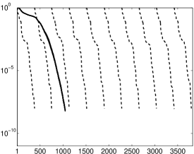
Fig. 1: Comparison of the performance of Algorithm 7.1 versus sequential applications of MINRES on the discretized Laplacian system with ten randomly generated right-hand sides. The solid black curve is actually the ten convergence curves for each right-hand side when solved by Algorithm 7.1 overlaid on one another. We see that in the case of these ten right-hand sides that block MINRES convergence for all ten systems is qualitatively the same. The black dashed curves are the convergence curves for each sequential application of MINRES for each right-hand side.

We begin by demonstrating the performance of the algorithm on the shifted Laplacian system with ten randomly generate right-hand sides. In Figure 1, we see that for these right-hand sides, the block MINRES algorithm converges in fewer iterations and less time.

We can also compare performance of our method versus sequential applications of MINRES for varying numbers of right-hand sides. We take as our first right-hand side the vector of all ones. If we have $p$ total right-hand sides, we take the remaining $p-1$ to be the first $p-1$ columns of the $\mathbf{I}_{n_{1}}$. In Figure 2, we plot for various $p$, the ratio between the iteration count of our method and the total iteration count for $p$ sequential applications of Matlab’s MINRES. For this experiment, we see a reduction in the ratio as $p$ increase, but the marginal benefit of adding each additional right-hand side diminishes for larger numbers of right-hand sides.

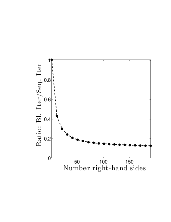
Fig. 2: For different numbers of right-hand sides, we plot the ratio between the number of iterations required by our block MINRES method and the sequential MINRES method to solve the system with multiple right-hand sides to a tolerance of $10^{-8}$. As the number of right-hand sides increases, the ratio decreases, i.e., our method requires fewer iterations than sequential MINRES.

We demonstrate that our removal of dependent vectors works as described. Of course, it is difficult to choose a pair of right-hand sides for which dependence will occur in later iterations. Thus, as a simple, easy-to-construct test, we chose the first right-hand side $\mathbf{e}_{1}$, as the first canonical basis vector. The second right-hand side is $\mathbf{A}\mathbf{e}_{1}$, the image of the first canonical basis vector, i.e., the first column of our coefficient matrix. This will result in dependence at the first iteration of our algorithm. As is shown in Figure 3, this leads to immediate convergence for that system when running block MINRES. Of course, this example is not likely to occur in practice. It merely demonstrates that the algorithm can handle dependence gracefully.

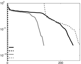
Fig. 3: Demonstration of the algorithm’s performance in the case that it encounters dependence. In this case, with the right-hand sides $\mathbf{e}_{1}$ and $\mathbf{A}\mathbf{e}_{1}$, dependence occurs at the first iteration. Since the first right-hand side is the solution to the second system, we get immediate convergence for the second system, and block MINRES continues for the other system, replacing the dependent vector with a random one.

We demonstrate how the relationship between the right-hand sides can affect the performance of block MINRES.

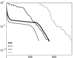
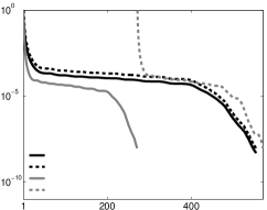
Fig. 4: Performance of block MINRES for different right-hand sides. In the figure on the left, the two right-hand sides are $\mathbf{b}_{1}=\mathbf{e}_{n_{1}}^{(1)}$ and $\mathbf{b}_{2}=\mathbf{1}$. In the figure on the right, $\mathbf{b}_{1}$ does not change, but $\hat{\mathbf{b}}_{2}=\mathbf{e}_{n_{1}}^{(2)}$.

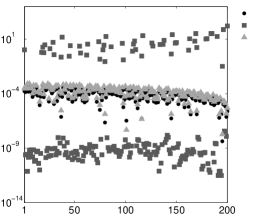
Fig. 5: Magnitude of the components of different right-hand-sides in the eigenspace spanned by the two hundred eigenvectors associated with the smallest magnitude eigenvalues.

We compared the performance of our block MINRES implementation with that of sequential runs of Matlab’s MINRES for $\mathbf{A}$ with three pairs of right-hand sides. For the first pair, let $\mathbf{b}_{1}=\mathbf{e}_{n_{1}}^{(1)}$ and $\mathbf{b}_{2}=\mathbf{1}$, the vector of all ones. For second pair of right-hand sides, we let $\hat{\mathbf{b}}_{1}=\mathbf{b}_{1}$ but change the second right-hand side by letting $\hat{\mathbf{b}}_{2}=\mathbf{e}_{n_{1}}^{(2)}$. In Figure 4, we show a comparison of convergence curves for these pairs of right-hand sides. We observe that exchanging $\mathbf{b}_{2}$ for $\hat{\mathbf{b}}_{2}$ degrades the performance of our Block MINRES implementation. Recall that the convergence of a Krylov subspace method for a symmetric system is completely determined by its eigenvalues and the decomposition of the initial residual in the eigenbasis. For an indefinite system, the eigenvalues closest to the origin cause a delay in convergence. In Figure 5, we decomposed the three right-hand sides in the eigenbasis and plotted the magnitudes of the $200$ eigencomponents associated to small eigenvalues. What we see is that almost all the components of $\mathbf{b}_{1}$ and $\mathbf{b}_{2}$ have similar magnitude while those of $\hat{\mathbf{b}}_{2}$ differ, with some being larger and others being smaller. Therefore, we hypothesize that a pair of right-hand sides that have strong components from different parts of the eigenspace might complement each other well.

We concoct some experiments to explore this line of thinking further. We construct two right-hand sides, each coming from the span of some subset of eigenvectors. We can further specify how many eigenvector components they have in common and see how this affects convergence.

Let $\left\{\mathbf{q}_{1},\mathbf{q}_{2},\ldots,\mathbf{q}_{n}\right\}$ be the orthonormal eigenvectors of $\mathbf{A}$, in ascending order according to the magnitude of their associated eigenvalues. We define the following subspaces,

$${\mathcal{Q}}_{S_{1}} = \text{span}\left\{\mathbf{q}_{1},\ldots,\mathbf{q}_{100}\right\}$$

$${\mathcal{Q}}_{S_{2}} = \text{span}\left\{\mathbf{q}_{101},\ldots,\mathbf{q}_{200}\right\}$$

$${\mathcal{Q}}_{L} = \text{span}\left\{\mathbf{q}_{n-200+1},\ldots,\mathbf{q}_{n}\right\}$$

In the first experiment, we construct both right-hand sides from eigenvectors associated only to eigenvalues of smaller magnitude, i.e., $\mathbf{b}_{1},\mathbf{b}_{2}\in{\mathcal{Q}}_{S_{1}}\oplus{\mathcal{Q}}_{S_{2}}$, such that a fixed number of eigenvectors are used to construct both vectors. We define the two right-hand sides

$$\mathbf{b}_{1}=\sum_{i=1}^{100+m}\alpha_{i}\mathbf{q}_{i}\mbox{\ \ and\ \ }\mathbf{b}_{2}=\sum_{i=100-m+1}^{200}\beta_{i}\mathbf{q}_{i}.$$ (19)

For $m=0$, $\mathbf{b}_{1}$ and $\mathbf{b}_{2}$ are orthogonal. For $m=1$, they both have components from $\mathbf{q}_{100}$ and $\mathbf{q}_{101}$ but are otherwise orthogonal. For $m=100$, both right-hand sides have components in all $200$ basis vectors of ${\mathcal{Q}}_{S_{1}}\oplus{\mathcal{Q}}_{S_{2}}$. For various values of $m$, we can test the performance of our algorithm. The coefficients $\left\{\alpha_{i}\right\}$ and $\left\{\beta_{i}\right\}$ are generated using Matlab’s rand() command. In order to avoid judging performance based on a specific random example (which may be an outlier), for each $m$ tested, we generated $100$ different pairs of right-hand sides. In Figure 6, we plot the average iteration counts over the $100$ tests for each $m$. Until $m=100$, we see little change in the iteration counts.

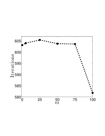
Fig. 6: Average performance of our method for pairs of right-hand sides built from the $200$ eigenvectors associated with the smallest magnitude eigenvalues, as described in (19). The right-hand sides have components from $2m$ common eigenvectors, but are otherwise orthogonal. For each $m$, the iteration counts and times are the averages of the results of tests for $100$ such pairs of right-hand sides.

We also performed the same experiment but constructed the two right-hand sides using eigenvectors from different parts of the spectrum. For different values of $m$, we define

$$\mathbf{b}_{1}=\sum_{i=1}^{200}\alpha_{i}\mathbf{q}_{i}+\underbrace{\sum_{i=n_{1}-200+1}^{n_{1}-200+m}\alpha_{i}\mathbf{q}_{i}}_{=0\mbox{\ when\ }m=0}\mbox{\ \ and\ \ }\mathbf{b}_{2}=\underbrace{\sum_{i=201-m}^{200}\beta_{i}\mathbf{q}_{i}}_{=0\mbox{\ when\ }m=0}+\sum_{i=n_{1}-200+1}^{n_{1}}\beta{i}\mathbf{q}_{i}.$$ (20)

When $m=0$, we have $\mathbf{b}_{1}\in{\mathcal{Q}}_{S_{1}}\oplus{\mathcal{Q}}_{S_{2}}$ and $\mathbf{b}_{2}\in{\mathcal{Q}}_{L}$ and they are orthogonal. For $m=1$ they share components from two eigenvectors ($\mathbf{q}_{200}$ and $\mathbf{q}_{n_{1}-200+1}$). For $m=200$, both right-hand sides have components from every basis vector of ${\mathcal{Q}}_{S_{1}}\oplus{\mathcal{Q}}_{S_{2}}\oplus{\mathcal{Q}}_{L}$. As in the previous experiment, 100 random pairs of right-hand sides were generated for each $m$, and the results averaged. Average iterations counts are shown in Figure 7. We see a quick drop in iterations at $m=25$ followed by an increase. Over all, mixing eigencomponents in this experiment produces a decrease in iteration counts.

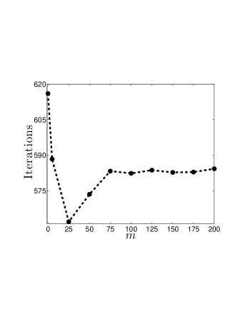
Fig. 7: Experiments constructed in the same as those shown in Figure 6 but now with pairs of right-hand sides constructed according to (20). Again the average iterations and times from tests for $100$ pairs of right-hand sides are given.

This is by no means a rigorous analysis of the convergence of a block method. These experiments only are meant to illustrate the variability of performance of a block method for different right-hand sides and provide some insight into this phenomenon.

9 Conclusions

We have presented an implementation of the block MINRES algorithm based on the band Lanczos process. This version is designed to perform many operations in a block fashion while maintaining the band Lanczos method’s easy-to-implement breakdown detection property. We provide not only a theoretical derivation of the algorithm but also a discussion of the practical implementation issues which need to be addressed to fully take advantage of the efficiencies which arise in a block method for symmetric systems. This variant of the block MINRES method handles dependence of block Krylov subspace basis vectors in a more straightforward manner than a block Lanczos-based algorithm. A software implementation in Matlab is provided at http://math.soodhalter.com/software.php.

References

- [1] José I. Aliaga, Daniel L. Boley, Roland W. Freund, and Vicente Hernández, A Lanczos-type method for multiple starting vectors, Mathematics of computation, 69 (2000), pp. 1577–1602.
- [2] James Baglama, Dealing with linear dependence during the iterations of the restarted block Lanczos methods, Numerical Algorithms, 25 (2000), pp. 23–36.
- [3] Allison H. Baker, John M. Dennis, and Elisabeth R. Jessup, On improving linear solver performance: a block variant of GMRES, SIAM J. Sci. Comput., 27 (2006), pp. 1608–1626.
- [4] Sebastian Birk and Andreas Frommer, A deflated conjugategate gradient method for multiple right-hand sides and multiple shifts, (In preparation).
- [5] J. Jack Dongarra and Aad J. van der Sten, High-performance computing systems: status and outlook, Acta Numer., 21 (2012), pp. 379–474.
- [6] Augustin A. Dubrulle, Retooling the method of block conjugate gradients, Electronic Transactions on Numerical Analysis, 12 (2001), pp. 216–233 (electronic).
- [7] Roland W. Freund, Computation of matrix Padé approximations of transfer functions via a Lanczos-type process, in Approximation theory VIII, Vol. 1 (College Station, TX, 1995), vol. 6 of Ser. Approx. Decompos., World Sci. Publ., River Edge, NJ, 1995, pp. 215–222.
- [8] Roland W. Freund and Manish Malhotra, A block QMR algorithm for non-Hermitian linear systems with multiple right-hand sides, in Proceedings of the Fifth Conference of the International Linear Algebra Society (Atlanta, GA, 1995), vol. 254, 1997, pp. 119–157.
- [9] Roland W. Freund and Noël M. Nachtigal, QMR: a quasi-minimal residual method for non-Hermitian linear systems, Numerische Mathematik, 60 (1991), pp. 315–339.
- [10] Anne Greenbaum, Iterative Methods for Solving Linear Systems, SIAM, Philadelphia, 1997.
- [11] Martin H. Gutknecht and Thomas Schmelzer, Updating the QR decomposition of block tridiagonal and block Hessenberg matrices, Applied Numerical Mathematics, 58 (2008), pp. 871–883.
- [12] , The block grade of a block Krylov space, Linear Algebra and its Applications, 430 (2009), pp. 174–185.
- [13] Mark Hoemmen, Communication-avoiding Krylov subspace methods, PhD thesis, University of California Berkeley, 2010.
- [14] Julian Langou, Iterative methods for solving linear systems with multiple right-hand sides, PhD thesis, CERFACS, France, 2003.
- [15] Damian Loher, Reliable nonsymmetric block Lanczos algorithms, PhD thesis, Diss. no. 16337, ETH Zurich, Zurich, Switzerland, 2006.
- [16] Dianne P. O’Leary, The block conjugate gradient algorithm and related methods, Linear Algebra and its Applications, 29 (1980), pp. 293–322.
- [17] Chris C. Paige and Michael A. Saunders, Solutions of sparse indefinite systems of linear equations, SIAM Journal on Numerical Analysis, 12 (1975), pp. 617–629.
- [18] Michael L. Parks, Kirk M. Soodhalter, and Daniel B. Szyld, Block krylov subspace recycling, In Preparation.
- [19] Mickaël Robbé and Miloud Sadkane, Exact and inexact breakdowns in the block GMRES method, Linear Algebra and its Applications, 419 (2006), pp. 265–285.
- [20] Axel Ruhe, Implementation aspects of band Lanczos algorithms for computation of eigenvalues of large sparse symmetric matrices, Mathematics of Computation, 33 (1979), pp. 680–687.
- [21] Yousef Saad, Iterative Methods for Sparse Linear Systems, SIAM, Philadelphia, Second ed., 2003.
- [22] Yousef Saad and Martin H. Schultz, GMRES: A generalized minimal residual algorithm for solving nonsymmetric linear systems, SIAM Journal on Scientific and Statistical Computing, 7 (1986), pp. 856–869.
- [23] Thomas Schmelzer, Block Krylov methods for Hermitian linear systems, master’s thesis, 2004.
- [24] Valeria Simoncini and Efstratios Gallopoulos, Convergence properties of block GMRES and matrix polynomials, Linear Algebra and its Applications, 247 (1996), pp. 97–119.
- [25] Valeria Simoncini and Daniel B. Szyld, Recent computational developments in Krylov subspace methods for linear systems, Numerical Linear Algebra with Applications, 14 (2007), pp. 1–59.
- [26] Kirk M. Soodhalter, A block MINRES algorithm based on the band lanczos method, Tech. Report 1301.2102v2, arXiv, 2013.
- [27] Brigitte Vital, Etude de quelques méthodes de résolution de problèmes linéaires de grande taille sur multiprocesseur, PhD thesis, Université de Rennes, 1990.