Gravitational conundrum? Dynamical mass segregation versus disruption of binary stars in dense stellar systems

Abstract

Upon their formation, dynamically cool (collapsing) star clusters will, within only a few million years, achieve stellar mass segregation for stars down to a few solar masses, simply because of gravitational two-body encounters. Since binary systems are, on average, more massive than single stars, one would expect them to also rapidly mass segregate dynamically. Contrary to these expectations and based on high-resolution Hubble Space Telescope observations, we show that the compact, 15–30 Myr-old Large Magellanic Cloud cluster NGC 1818 exhibits tantalizing hints at the $\gtrsim 2\sigma$ level of significance ($>3\sigma$ if we assume a power-law secondary-to-primary mass-ratio distribution) of an increasing fraction of F-star binary systems (with combined masses of 1.3–$1.6M_{\odot}$) with increasing distance from the cluster center, specifically between the inner 10 to 20^′′ (approximately equivalent to the cluster’s core and half-mass radii) and the outer 60 to 80^′′. If confirmed, this will offer support of the theoretically predicted but thus far unobserved dynamical disruption processes of the significant population of ‘soft’ binary systems—with relatively low binding energies compared to the kinetic energy of their stellar members—in star clusters, which we have access to here by virtue of the cluster’s unique combination of youth and high stellar density.

1 Introduction

In the absence of gas, gravity is the dominant force driving the dynamical evolution of stellar systems. Its effects are most easily discernible in the dense cores of massive stellar clusters. Because of the close proximity of stars within a cluster, most stars experience significant gravitational perturbations, close encounters, and occasionally physical collisions. A cluster’s most massive stars are almost always found in the inner regions (e.g., de Grijs et al. 2002a,b,c; Gouliermis et al. 2004; and references therein). However, the origin of this observed mass segregation at early times and the dynamical timescales required to reach energy equipartition of at least the most massive stars seem mutually exclusive, particularly so in the youngest open clusters (Bonnell & Davies 1998). These arguments are based on the results of numerical (‘$N$-body’) simulations under the assumption of uniform, homogeneous initial conditions, i.e., taking Plummer spheres as their starting points. This apparent conflict has led to numerous studies that explored whether massive stars will most likely form in the centers of clusters, i.e., through a process coined ‘competitive accretion,’ or if they might slowly sink to the cluster core owing to gravitational interactions and energy exchange with other cluster stars, commonly known as ‘dynamical mass segregation.’ If competitive accretion were at work, this would possibly require an environmental dependence of the stellar initial mass function (IMF) on small spatial scales (referred to as ‘primordial mass segregation’).

Both observations and theoretical arguments suggest that young star clusters form as highly substructured entities. Observationally, however, young clusters seem to homogenize on timescales of $<2$ Myr (Cartwright & Whitworth 2004; Schmeja et al. 2008). Simulations imply that this could only happen if clusters are formed dynamically cool (Goodwin et al. 2004; Allison et al. 2009). Several teams have, therefore, recently performed $N$-body simulations to explore the earliest phases of cluster evolution (McMillan et al. 2007; Allison et al. 2009, 2010; Moeckel & Bonnell 2009a,b; Yu et al. 2011). They find that initially cool clusters undergo rapid dynamical mass segregation for stellar masses down to a few solar masses and within a few million years.

Observations of local areas of active star formation indicate that almost all stars form in binary or higher-order multiple systems, across the full stellar mass range (e.g., Kouwenhoven et al. 2005, 2007; Raghavan et al. 2010; Sana & Evans 2011). These systems are initially located so close to each other that they interact, destroying some multiple systems and swapping partners with others. Such systems could, therefore, significantly affect the dynamical evolution of a cluster: hard binaries become harder while soft binaries tend to become softer. The former will have a higher impact on the dynamical cluster evolution than their equivalent single stars because of their increased cross section for dynamical interactions and the combined mass of the binary members. However, the initial binary fractions, $f_{\rm bin}$, in dense star clusters are largely unknown; $f_{\rm bin}\equiv B/(S+B+\cdots)$, where $S$ and $B$ represent single and binary systems, respectively, while the ellipsis implies inclusion of higher-order multiples. Binary systems are characterized by mass-ratio distributions $q\equiv m_{2}/m_{1}$, where $m_{1}$ and $m_{2}$ are the primary and secondary stellar masses, respectively, and $m_{2}\leq m_{1}$. Since binary systems, and in particular systems characterized by $q$ relatively close to unity, are on average more massive than single stars in a given stellar population, they are expected to play a more significant role in the dynamical evolution of their host cluster. In view of the recent simulations referred to above (Allison et al. 2009; Yu et al. 2011), one would therefore expect these systems to rapidly mass segregate dynamically.

2 Binary systems in young star clusters

The binary fractions in distant, massive clusters are challenging to study observationally, although analysis of their color–magnitude diagrams (CMDs) using artificial-star tests is gaining ground (e.g., Zhao & Bailyn 2005; Sollima et al. 2007; Davis et al. 2008; Hu et al. 2010; Milone et al. 2012). However, almost all clusters to which this technique has been applied thus far are old stellar systems in the Milky Way. Unfortunately, there are no nearby young massive clusters, with the possible exceptions of the 4–5 Myr-old massive cluster Westerlund 1 and the red-supergiant-dominated clusters near the Galactic Center (e.g., Figer et al. 2006; Davies et al. 2007, 2012). However, all of these young Galactic clusters are affected by significant foreground extinction and/or forbidding environmental conditions, so that significant external gravitational effects may have already altered their stellar make-up, thus preventing us from assessing the importance of cluster-internal dynamics.

A number of teams have begun to explore the binary fractions in the young ‘populous’ clusters in the much more distant Large Magellanic Cloud (LMC; e.g., Elson et al. 1998). We developed and validated an artificial-star test technique (Hu et al. 2010, 2011) to assess the binary fractions in dense environments, i.e., by examining a population’s ensemble properties. Here, we present a detailed study of the radial dependence of the fraction of binary systems characterized by $q\geq 0.55$ in the young (15–30 Myr-old), very compact (core, effective radii: $R_{\rm core}=2.1\pm 0.4$ pc, $R_{\rm eff}=5.4$ pc; at the LMC’s distance, $1^{\prime\prime}\equiv 0.26$ pc), massive [$M_{\rm cl}=(1.3-2.6)\times 10^{4}M_{\odot}$] cluster NGC 1818 using high-resolution Hubble Space Telescope (HST) observations (cf. de Grijs et al. 2002a; Mackey & Gilmore 2003). In Hu et al. (2010) we estimated the overall binary fraction of F-type stars (1.3–$1.6M_{\odot}$) in NGC 1818 at $\sim 0.35$, assuming a flat mass-ratio distribution for $q>0.4$, which is consistent with a total binary fraction of 55 to 100%.

3 Hubble Space Telescope observations and analysis

We used data obtained with the Wide-Field and Planetary Camera-2 (WFPC2) on board the HST as part of General Observer (GO) program GO-7307 (PI Gilmore). WFPC2 contains four chips (each composed of $800\times 800$ pixels), a Planetary Camera (PC) and three Wide-Field (WF) arrays. The PC’s field of view is approximately $34\times 34$ arcsec² ($0.0455^{\prime\prime}$ pixel^-1) and each of the WF chips has a field of view of approximately $150\times 150$ arcsec² ($0.097^{\prime\prime}$ pixel^-1). We obtained WFPC2 images in the F555W (henceforth $V$) and F814W ($I$) broad-band filters, with the PC centered on both the cluster core and on a location offset by approximately $40^{\prime\prime}$ to the south west, i.e., roughly pointing at the cluster’s half-mass radius at that location (de Grijs et al. 2002a). Our exposures in which the PC is located on the cluster center consist of sets of deep (140 and 300 s for each individual image in F555W and F814W, respectively) and shallow (5 and 20 s for each equivalent image, respectively) images. The observations centered on the cluster’s half-mass radius are characterized by individual exposure times of 800, 800, and 900 s in both filters. The data reduction has been described by Hu et al. (2010, 2011). Here we use the same reduced data set.

To explore the radial dependence of the cluster’s binary fraction, we first obtained a new estimate of the cluster center by fitting Gaussian profiles to the number-density distributions along both the right ascension ($\alpha_{\rm J2000}$) and declination ($\delta_{\rm J2000}$) axes, covering the cluster’s area inside $2R_{\rm eff}$ by 10 bins in each coordinate direction. The resulting center coordinates, expressed in the WFPC2 world coordinate system, are $\alpha_{\rm J2000}=05^{\rm h}04^{\rm m}13.2^{\rm s},\delta_{\rm J2000}=–66^{\circ}26^{\prime}03.7^{\prime\prime}$. The cluster’s azimuthally averaged number-density profile disappears into the (approximately constant) background noise at a radius $R=(72.7\pm 0.3)^{\prime\prime}$.

Ideally, without binaries and observational errors, all stars in a cluster that have evolved through the pre-main-sequence phase should occupy a single isochrone, because they have (approximately) the same age and metallicity. However, in practice, the cluster’s main sequence is contaminated by field stars. Therefore, we statistically subtracted background stars (for full details, see Hu et al. 2010). More importantly, main sequences in observational CMDs tend to exhibit a non-negligible broadening caused by the presence of true binary/multiple systems, compounded by a combination of photometric errors and chance line-of-sight superpositions (‘blending’). Photometric errors cause a symmetrical broadening of the main sequence, assuming that the magnitude errors are approximately Gaussian (symmetric with respect to the mean); in our analysis we adopted an exponential error distribution with increasing magnitude (Hu et al. 2010). However, chance superpositions and the presence of a population of physical binary systems both introduce offsets to the brighter, redder side with respect to the best-fitting isochrone. Because distinguishing between superpositions and physical binaries based on CMD morphological analysis alone is all but impossible, we performed extensive Monte Carlo tests to generate artificial-star catalogs. We adopted a range of binary fractions (as well as mass-ratio distributions; see Sect. 4) and compared the spreads of real and artificial stars with respect to the best-fitting isochrone.

To simulate the effects of chance superpositions and to allow us to assess the radial dependence of the cluster’s binarity, we randomly distributed a minimum of 640,000 artificial stars, drawn from a Kroupa (2002)-type stellar IMF covering the stellar mass range from 0.08 to $50M_{\odot}$, on the spatial distribution diagram of the real stars (for procedural details, see Hu et al. 2010). If the distance between an artificial star and any real star is $\leq 2$ pixels (corresponding to the minimum separation allowing us to detect them as separate objects), we assume it to be blended (see Hu et al. 2011). Artificial stars are not allowed to blend with each other. Fig. 1a shows the resulting blending fraction as a function of both position within the cluster and the stellar magnitude range sampled. We thus proceeded to statistically correct the observational NGC 1818 CMD for the effects of stellar blends. We also determined and corrected our data for the effects of sample incompleteness as a function of radius within the cluster (see Fig. 1b). Note that the apparent peak near $V=24$ mag in Fig. 1a has been induced artificially by the effects of incompleteness, as can be deduced from a comparison with Fig. 1b.

In addition, based on extensive tests (see Hu et al. 2010), we found that any residual background population in the region in CMD space of interest (see below) is negligible: we derived a systematic error of $<3$%. This fraction is based on a comparison of the number of residual background stars with the number of roughly equal-mass binary systems in the cluster’s CMD.

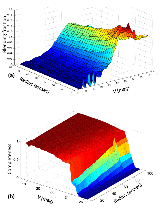
Figure 1: (a) Fraction of stellar blends in and (b) sample completeness of the NGC 1818 CMD as a function of radius from the cluster center and stellar magnitude range.

Star clusters containing equal-mass binary systems will exhibit an upper envelope to the region in CMD space occupied by binaries which is 0.752 mag brighter than the locus of the single-star main sequence, with unequal-mass binaries occupying the space between both sequences. For our analysis, we selected the region in color–magnitude space where the single-star main sequence is shallowest and our sample is $>85$% complete: for $V<20$ and $V>22$ mag, the CMD is too steep to easily disentangle single from binary stars and blends. In addition, toward fainter magnitudes, photometric errors start to dominate any potential physical differences, and field-star contamination becomes increasingly important outside of the region adopted for our binarity analysis.

4 Mass-ratio distributions and radial dependences

The remaining free parameter of importance for our analysis is the mass-ratio distribution, expressed as ${\rm d}N/{\rm d}q\propto q^{-\alpha}$, where $\alpha>0\;(\alpha<0)$ implies that the mass-ratio distribution is dominated by low- (high-)mass-ratio binary systems. Previous studies (Kouwenhoven et al. 2005, 2007; Reggiani & Meyer 2011) suggest that $\alpha\in$ [0.0, 0.4] is typical for binary systems in low-density environments. We will show below that this also appears a reasonable choice for the binary systems in NGC 1818 and its surrounding field. Here, we adopt both $\alpha=0.0$ and 0.4 to illustrate that the choice of mass-ratio distribution does not introduce any significant additional uncertainties in our analysis of the cluster’s radial binary fraction. For a given mass-ratio distribution, the best-fitting binary fraction within a given radius (i.e., a cumulative binary fraction covering the full radial range from the cluster center to the radius of interest, a choice driven by the need to base our results on statistically significant numbers of stars) is given by statistical $\chi^{2}$ analysis.

4.1 Radial trends

We generated artificial CMDs based on Padova stellar isochrones (Bressan et al. 2012) that are representative of the cluster’s age and (roughly solar) metallicity, and characterized by (18) binary fractions ranging from $f_{\rm bin}=0.05$ to 0.90 in steps of 0.05. For the data covering the range from the cluster center to a given radius, we determined the full two-dimensional CMD’s $\chi^{2}$ statistic associated with these variable binary fractions, i.e., we quantitatively compared the observed and artificial CMDs while only allowing a single free parameter, $f_{\rm bin}$. For practical convenience, we used a parabolic curve to describe the dependence of the $\chi^{2}$ value of the best fit on the input binary fraction to obtain both the minimum value, $\chi^{2}_{\rm min}$, and the $1\sigma$ uncertainties. The latter correspond to the difference between the binary fractions characterized by $\chi^{2}_{\rm min}$ and $\chi^{2}_{\rm min}+1$ (Avni 1976; Wall 1996; applicable to single-parameter fits). The resulting binary fractions as a function of radius in the cluster, in the restricted magnitude range from $V=20$ to 22 mag, and for our two choices of $\alpha$ are shown in Fig. 2 (top: $\chi^{2}$ landscape for $\alpha=0.0$ and 0.4; bottom: corresponding radial binary fractions). Our main result is that the binary fraction shows hints of an increase out to $40^{\prime\prime}$, irrespective of the value of $\alpha\in$ [0.0, 0.4] adopted. Our method is sensitive to binary systems with $q\geq 0.55$.

Note that the error bars associated with each successive data point as a function of increasing radius are not statistically independent. Each new data point includes the stars in our selected CMD parameter space covered by the data points at smaller radii. The latter are combined with the stars located at radii beyond those covered by the previous data point and up to the radius of interest to yield the cumulative binary fraction at that radius. Specifically, for $R\leq 10^{\prime\prime}$ and in the magnitude range covered by our Monte Carlo simulations, the number of stars used for the $\chi^{2}$ minimization is 92, increasing to 263, 400, 517, 614, 697, 782, and 858 for every successive cumulative fraction at radii that increase in steps of $10^{\prime\prime}$. The $\chi^{2}$ distribution as a function of (simulated) binary fraction is very well described by a parabolic function, with a clearly defined minimum, for all radial ranges.

This, combined with the notion that we are using cumulative radial distributions to base our conclusions on, leads us to suggest that the apparent increasing trend in binary fraction with increasing radius may be real. At the very least, we can robustly rule out a decreasing trend as would be expected if dynamical mass segregation were the main mechanism driving the radial distribution of the stellar binary fraction, even at (or despite) the cluster’s young age. This would require a conspiracy between the radial distributions of single and binary systems that is not supported by the observations. Because of the correlated error bars between successive data points, combined with the well-defined $\chi^{2}_{\rm min}$ as a function of $f_{\rm bin}(\leq R)$, Fig. 2 offers tantalizing hints of the reality of an increasing fraction of binary systems from the cluster center outward. If the binary fraction were roughly constant as a function of radius, in a cumulative distribution such as that shown here, we would expect to see clearly discernible random changes in the slope of the distribution between successive data points instead of the small yet sustained increase potentially detected here.

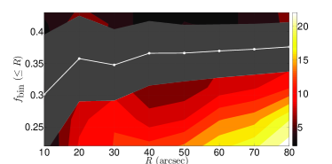
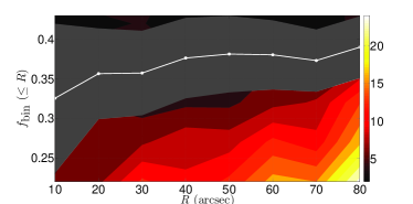
Figure 2: Cumulative binary fractions in NGC 1818 as a function of radius from the cluster center, for power-law indices $\alpha=0.0$ (top left and bottom left) and $\alpha=0.4$ (top right and bottom right), based on $\chi^{2}$ minimization and for $q\geq 0.55$. The color scheme is representative of the $\chi^{2}$ values resulting from our comparison between the observational data and our Monte Carlo realizations, with darkest red referring to the lowest values. The loci of the minimum $\chi^{2}$ values and the $1\sigma$ uncertainties (grey) are also indicated.

4.2 Statistical analysis

Rather than merely relying on hints, we can make use of well-established and robust frequentist statistical methods to place our results on a proper statistical footing. Unfortunately, application of statistical analysis to the cumulative $f_{\rm bin}$ distributions of Fig. 2 is highly complex and, in fact, poorly understood. Therefore, we proceed by employing individual, non-overlapping radial ranges for our statistical analysis, so that the error bars and data points at successive radii are independent.

Nevertheless, our statistical interpretation of the results is not straightforward, even by making this simplification, because of the two-step process we employed to obtain the best-fitting $f_{\rm bin}$ values. For every radial range, we independently obtain the $\chi^{2}$ statistic associated with a set of input $f_{\rm bin}$ values, employing independently generated random seeds in our Monte Carlo simulations. For a given $f_{\rm bin}$, the resulting $\chi^{2}$ value is thus based on our analysis of a statistically significant number of stars in color–magnitude space (for the actual numbers of stars used, see Table 1). In the second step, we fit a parabolic function to the distribution of $\chi^{2}$ values as a function of $f_{\rm bin}$ to obtain the mean $\chi^{2}$ value and its $1\sigma$ uncertainty (as defined in Section 4.1). The $\chi^{2}$ distribution at a given radius is well represented by a symmetric parabolic function.

Our aim is not to ascertain the reality (or otherwise) of a radial trend, but to determine whether the means of the $f_{\rm bin}$ values in selected (inner) cluster regions are statistically different from non-overlapping regions elsewhere in the cluster, given the error bars. In essence, therefore, for each assessment we need to compare two samples composed of 18 data points each, i.e., the $\chi^{2}$ values for each of the 18 input $f_{\rm bin}$ values for a given radial range, corresponding to a total sample size of 36 for the two distributions being investigated. Since the number of data points is smaller than approximately 50–60 (the rule-of-thumb lower limit for adoption of normal distributions; but one should realize that each of these data points itself was derived on the basis of a much larger intrinsic sample size), methods based on normal distributions could prove inadequate because of small-number statistics. Instead, the Student’s $t$ distribution represents the most appropriate approach to calculate score values associated with different levels of significance. We compare the resulting $t$ scores to the relevant values for a $t$ distribution with $(18-1)$ degrees of freedom.

The statistical analysis method we have chosen to adopt is a standard hypothesis-based comparison of two means that follow Gaussian distributions (e.g., Montgomery 2001, his Chapter 2; Martinez & Martinez 2007, their Chapter 6). More sophisticated statistical tests that analyze the mutual differences at different radii are left for future work.

In the current context, the Student’s $t$ test is formalized as follows in a statistically robust manner. Let $\mu_{1}$ and $\mu_{2}$ denote the means of two different minimizations derived from the $\chi^{2}$ fits, with standard deviations $\sigma_{1}$ and $\sigma_{2}$, respectively. We want to connect these expressions to a statistical value that can be used to test whether or not the means are statistically equal. In its most general form, the two-sample $t$ test is well approximated by

$$t_{0}=\frac{\mu_{1}-\mu_{2}}{\sqrt{\frac{\hat{\sigma}_{1}^{2}}{n_{1}}+\frac{\hat{\sigma}_{2}^{2}}{n_{2}}}},$$ (1)

with

$$\nu=\frac{\left(\frac{\hat{\sigma}_{1}^{2}}{n_{1}}+\frac{\hat{\sigma}_{2}^{2}}{n_{2}}\right)^{2}}{\frac{\large(\hat{\sigma}_{1}^{2}/n_{1}\large)^{2}}{n_{1}-1}+\frac{\large(\hat{\sigma}_{2}^{2}/n_{2}\large)^{2}}{n_{2}-1}}$$ (2)

degrees of freedom. In these expressions, $\hat{\sigma}^{2}$ denotes the maximum-likelihood estimation of the sample variance, computed by

$$\hat{\sigma}^{2}=\frac{\sum_{i=1}^{n}(x_{i}-\mu)}{n-1}.$$ (3)

To connect the sample variance with the standard deviation derived from our $\chi^{2}$ minimization, we assume that we can draw data points from the distribution derived using $\sigma$. The sample variance of those data points would be given by $\hat{\sigma}$. Also note that the denominator of the $t$-test formalism contains an expression of the form $\hat{\sigma}^{2}/n$. We can transform this equation as

$$\frac{\hat{\sigma}^{2}}{n}=\frac{\sigma^{2}\hat{\sigma}^{2}}{\sigma^{2}n}=\frac{\sigma^{2}\sum_{i=1}^{n}(x_{i}-\mu)}{n\sigma^{2}(n-1)}=\frac{\sigma^{2}\chi_{n-1}^{2}}{n(n-1)}.$$ (4)

Inserting this transformation into the expression for a $t$ test gives

$$t_{0}=\frac{\mu_{1}-\mu_{2}}{\sqrt{\frac{\sigma_{1}^{2}\chi_{n_{1}-1}^{2}}{n_{1}(n_{1}-1)}+\frac{\sigma_{2}^{2}\chi_{n_{2}-1}^{2}}{n_{2}(n_{2}-1)}}}.$$ (5)

This expression only contains values that are derived from the $\chi^{2}$ minimization. Moreover, we do not need to compute sample data points, which would be derived from the associated Gaussian distributions. For the degrees of freedom, we can likewise substitute the expression for $\hat{\sigma}^{2}$ to give

$$\nu=\frac{\left(\frac{\sigma_{1}^{2}\chi_{n_{1}-1}^{2}}{n_{1}(n_{1}-1)}+\frac{\sigma_{2}^{2}\chi_{n_{2}-1}^{2}}{n_{2}(n_{2}-1)}\right)^{2}}{\frac{\large(\sigma_{1}^{2}\chi_{n_{1}-1}^{2}/n_{1}\large)^{2}}{(n_{1}-1)^{3}}+\frac{\large(\sigma_{2}^{2}\chi_{n_{2}-1}^{2}/n_{2}\large)^{2}}{(n_{2}-1)^{3}}}.$$ (6)

Although this derivation does not constitute a formal proof—a more rigorous analysis would have to include a full Taylor-series expansion—this is a convenient approach which gives credence to our results, since it allows us to connect the number of degrees of freedom for the $\chi^{2}$ fits used in our minimization to that used for the $t$ test we need to use for the statistical analysis. Given this paradigm, we can then test the hypothesis as to whether or not the means of the binary fractions are statistically equal at different radii by applying the $t$-test methodology with associated thresholds.

Under these conditions, let $r_{i}$ denote radii at various distances from the cluster center, where $i$ runs from the innermost radial bin to the bin which encompasses the cluster’s outermost radius, here set to $R=80^{\prime\prime}$ for convenience. Let $\mu_{i}$ and $\sigma_{i}$ denote the means and standard deviations at the respective radii. To test if the mean numbers of binary fractions at different radial ranges exhibit statistical differences with respect to the outermost bin (denoted by the subscript ‘$80^{\prime\prime}$’), we express a (one-sided) hypothesis test in the form

$$H_{0}:\mu_{80^{\prime\prime}}=\mu_{i}\mbox{ versus }H_{1}:\mu_{80^{\prime\prime}}>\mu_{i}.$$ (7)

The equation that defines values with which the hypothesis can be tested is

$$t_{0}=\frac{\mu_{80^{\prime\prime}}-\mu_{i}}{\sqrt{\frac{\sigma_{80^{\prime\prime}}^{2}}{n_{80^{\prime\prime}}}+\frac{\sigma_{i}^{2}}{n_{i}}}}.$$ (8)

The $t$ scores are expressed in units of the data set’s ‘quantiles,’ where significance levels of 0.05 and 0.01 correspond to a difference of 2 or 3 standard deviations between means, respectively. In other words, significances of 0.10, 0.05, and 0.01 represent confidence intervals of 90, 95, and 99%, respectively. Using this methodology, we compute values for the test statistic and compare these with threshold values derived from the inverse value of the cumulative probability-density function of a Student’s $t$ distribution. If the test value is less than the threshold, statistical theory implies that we must accept the null hypothesis ($H_{0}$). Otherwise, we are led to reject the null hypothesis and accept the alternative ($H_{1}$).

Table 1: Student’s $t$ scores (expressed in units of the sample’s quantiles) and levels of significance (‘Sign.’; lower limits) for radial differences in the mean binary fractions, $\mu_{i}$. Significance levels usually considered statistically conclusive (i.e., $>2\sigma$) are rendered in bold-face font. The threshold $t$ scores applicable to a one-sided hypothesis test for the 0.10, 0.05, and 0.01 levels of significance are 1.30, 1.73, and 2.55, respectively.

Radial range (′′)			$N$(stars)			Student’s $t$ score
Inner	Outer		Inner	Outer		$\alpha=0$	Sign.	$\alpha=0.4$	Sign.
0–10	70–80		92	76		2.08	0.05	3.25	0.01
0–10	60–80		92	161		3.19	0.01	3.36	0.01
0–10	40–80		92	341		2.37	0.05	4.18	0.01
0–20	60–80		263	161		2.26	0.05	1.59	0.10
0–20	40–80		263	341		0.79	—	2.26	0.05
0–40	40–80		517	341		1.55	0.10	2.53	0.05

Table 1 lists the $t$ scores for the statistical differences in the mean values between the binary fraction representative of the cluster’s presumably unevolved outer regions (out to $R=80^{\prime\prime}$) and those in other, more central radial ranges considered, for both the flat mass-ratio distribution and that characterized by a power-law index $\alpha=0.4$. For both assumptions of the mass-ratio distribution, the thresholds for the $t$ scores, assuming a one-sided hypothesis test (as applied here), are 1.30, 1.73, and 2.55 for the 0.10, 0.05, and 0.01 levels of significance, respectively. We can interpret these results as follows. Depending on the radial bin size and to some extent also on the value adopted for the power-law exponent $\alpha$, it appears that the difference between the mean binary fractions in the inner 10 to 20^′′ (roughly corresponding to the cluster’s core and half-mass radii, respectively) and the outer 60 to 80^′′ is $\sim 2\sigma$ (standard deviations), except for the differences in the means between the inner 10^′′ and any of the outer radial ranges for the assumption of a power-law mass-ratio distribution. If the latter assumption holds, the mean binary fraction in the inner 10^′′ is statistically $\gtrsim 3\sigma$ different from any of our adopted radial ranges that include the cluster’s outermost radius, $R=80^{\prime\prime}$. The significance levels for the power-law mass-ratio distribution are systematically higher than the equivalent values for a flat mass-ratio distribution. We emphasize that these statistical results properly account for both the extents of the associated error bars and the relevant sample sizes.

4.3 Additional support

We subsequently and independently verified the reality of the suggested rising trend as a function of radius by employing a poor man’s approach to the derivation of the radial binary fractions: we determined the main-sequence ridgeline and its dispersion, $\sigma_{\rm ms}$, as well as the expected locus of the equal-mass binary sequence. We split up the available parameter space into ‘single-star’ and ‘binary’ regimes. The single-star regime was delineated by the adopted minimum and maximum magnitudes, and the main-sequence ridgeline $\pm 3\sigma_{\rm ms}$ (to account for the photometric errors). For binary stars, we used the same limiting magnitudes and adopted the region from the main-sequence ridgeline $+3\sigma_{\rm ms}$ to the theoretical equal-mass binary sequence $+3\sigma_{\rm ms}$ (see Fig. 3a). We then proceeded by counting stars in both areas to obtain a lower limit to the actual binary fraction, which exhibited a similar increase as a function of $R$ (see Fig. 3b), flattening out at $31.0\pm 1.9$% for $R\geq 72.7^{\prime\prime}$, where the cluster profile disappears into the background noise.

Although the zero-point calibration of this simple method does not take into account the effects of blending, the general trend is robust for $q>0.6$ (Hu et al. 2010; cf. Elson et al. 1998 for validation of the $q$ cut). This strengthens the result from our more sophisticated Monte Carlo approach, so that we conclude that the increasing binary fraction as a function of radius from the cluster center is indeed most likely realistic. Note that if this trend were due to incorrect background corrections, it would follow the cluster’s radial density profile very closely. This is not supported by our results.

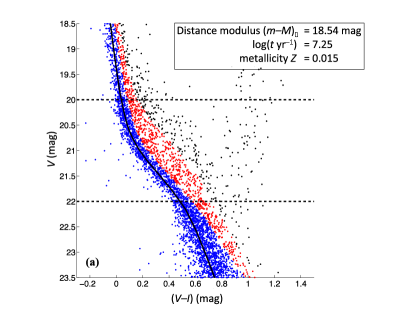
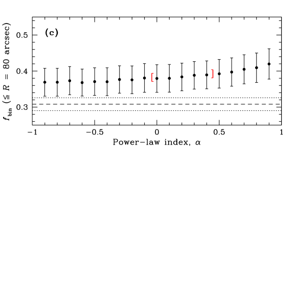
Figure 3: (a) NGC 1818 CMD, including the best-fitting isochrone (parameters indicated), where we have indicated the regions used for our poor-man’s approach. Blue: single-star area, red: ‘binaries;’ black: discarded stars outside our selection regions. (b) Cumulative binary fraction in NGC 1818 as a function of radius from the cluster center, based on our isochrone-fitting approach. (c) Total binary fraction as a function of power-law index, $\alpha$, adopted for the full cluster region within $R=80^{\prime\prime}$ and for binary systems characterized by $q\geq 0.55$. The dashed and dotted lines indicate the (lower limit to the) binary fraction and the $1\sigma$ error bars, respectively, obtained from our isochrone-fitting approach. The (red) square brackets indicate the range in $\alpha$ adopted.

Finally, we applied our fitting routines to the full NGC 1818 CMD—within the restricted magnitude range where binary systems are most clearly discernible and for $R\leq 80^{\prime\prime}$—and examined the effects of our choice of mass-ratio distribution by varying $\alpha$: see Fig. 3c. We also included the lower limit obtained from our simple isochrone-fitting analysis. This comparison shows that our choice of $\alpha\in$ [0.0, 0.4] is reasonable; in this range of $\alpha$, the cluster’s derived global binary fraction is approximately constant within the uncertainties. The binary fraction obtained from our isochrone-fitting approach returns a lower limit, because some binary systems inevitably pollute the single-star regime.

5 Implications

Numerical simulations based on realistic initial conditions (i.e., initial substructure and initially cool dynamics) suggest that dynamical mass segregation, at least of the most massive stars, is likely to happen in a crossing time, which is equivalent to the free-fall time defined by the cluster’s gravitational potential. In de Grijs et al. (2002b), we estimated that NGC 1818 is $\sim$5–30 crossing times old. Hard binary stars may accelerate dynamical mass segregation significantly, since close encounters between binary systems and between binaries and single stars are very efficient (e.g., Parker et al. 2011).

Stars in the stellar mass range targeted in our study, 1.3–$1.6M_{\odot}$ (Hu et al. 2010), are not expected to have already reached a state close to energy equipartition on a cluster-wide scale: the cluster’s half-mass relaxation time for these masses is $\geq 500$ Myr (de Grijs et al. 2002b). This implies that the process of cluster-wide dynamical mass segregation is likely still fully underway in NGC 1818. Yet, contrary to dynamical expectations (based on initial conditions using Plummer spheres), we found a tantalizing hint of an increasing fraction of binary systems in NGC 1818 from the innermost (core) radius where we could detect such systems reliably ($\sim 10^{\prime\prime}$) out to approximately its half-light radius. This is surprising and, if confirmed independently, flies in the face of previous results for the same cluster.

A fraction of 35% ($\pm 5$%) of roughly similar-mass binaries (with $17.5<m_{\rm F555W}<20.3$ mag, corresponding to $2.0<m_{1}<5.5M_{\odot}$) was reported in the center of NGC 1818 by Elson et al. (1998), decreasing to 20% ($\pm 5$%) beyond $\sim 3R_{\rm core}$. However, our analysis—in particular based on Fig. 1a—has shown that their result can be attributed to the effects of blending and the near-vertical extent of the stellar main sequence for their adopted magnitude range, which mask the real underlying signal. In addition, we already reported a clear detection of the effects of mass segregation in NGC 1818 for stars with masses $\geq 1.6M_{\odot}$ (de Grijs et al. 2002b), under the assumption that all stars in our sample were single stars. Despite the (sizeable but correlated) error bars associated with our main result shown in Fig. 2, Elson et al.’s (1998) suggested trend cannot be accommodated by the blending-corrected distribution of single and binary stars in this cluster.

Since most current theories of binary formation (either dynamically or primordially) do not explicitly depend on gas or stellar density, we have no reason to expect a priori that cluster core environments feature intrinsically lower binary fractions ab initio. As such, we are left to conclude that the suggested trend of an increasing fraction of F-star binary systems with increasing radius from the cluster center, if confirmed to be real, may be caused by early dynamical evolution, i.e., the rapid dissolution of binary systems due to two-body encounters. The radial dependence of the binary fraction in dense star clusters has never before been determined for clusters as young as NGC 1818. We are currently extending our analysis to other young clusters in the LMC (C. Li et al., in prep.). Preliminary results for the equivalently young but much more sparsely populated cluster NGC 1805 indicate a radial trend of greater significance than for NGC 1818, and which is opposite to the radially increasing fraction of F-type binaries suggested here (as expected from dynamical arguments).

If our reported $\gtrsim 2\sigma$ difference in the mean binary fractions in NGC 1818 between the inner and outer $\sim 20^{\prime\prime}$ stands the test of further scrutiny, we need to compare the timescale governing dynamical mass segregation with the expected binary disruption rate so as to understand this radial dependence. Given the cluster’s age in units of its crossing time (de Grijs et al. 2002b), we expect that its initial binary population should have been altered by dynamical interactions. In particular, the destruction of soft (i.e., wide) binaries due to close encounters—on timescales of order the crossing time or less (Heggie 1975; Parker et al. 2009)—should be well underway, at least in the cluster’s core region; distant encounters are unimportant for the disruption of close binaries (Heggie 1975). In addition, as Heggie (1975) already pointed out, soft binaries are expected to be more centrally concentrated than single stars. Therefore, our observed radial dependence suggests that we are seeing the relatively ‘hard’ binary systems that have survived and may have been hardened by dynamical encounters. This would offer unprecedented evidence in support of theoretically predicted dynamical processes governing star cluster evolution, which we now have access to by virtue of the unique combination of youth and high stellar density of NGC 1818.

References

- Allison et al. (2009) Allison, R. J., Goodwin, S. P., Parker, R. J., et al. 2009, ApJ, 700, L99
- Allison et al. (2010) Allison, R. J., Goodwin, S. P., Parker, R. J., Portegies Zwart, S. F., & de Grijs, R. 2010, MNRAS, 407, 1098
- Avni (1976) Avni, Y. 1976, ApJ, 210, 642
- Bonnell & Davies (1998) Bonnell, I. A., & Davies, M. B. 1998, MNRAS, 295, 691
- Bressan et al. (2012) Bressan, A., Marigo, P., Girardi, L., et al. 2012, MNRAS, 427, 127 (http://stev.oapd.inaf.it/cmd)
- Cartwright & Whitworth (2004) Cartwright, A., & Whitworth, A. P. 2004, MNRAS, 348, 589
- Davies et al. (2007) Davies, B., Figer, D. F., Kudritzki, R.-P., et al. 2007, ApJ, 671, 781
- Davies et al. (2012) Davies, B., de La Fuente, D., Najarro, F., et al. 2012, MNRAS, 419, 1860
- Davis et al. (2008) Davis, D. S., Richer, H. B., Anderson, J., et al. 2008, AJ, 135, 2155
- de Grijs et al. (2002a) de Grijs, R., Johnson, R. A., Gilmore, G. F., & Frayn, C. M. 2002a, MNRAS, 331, 228
- de Grijs et al. (2002b) de Grijs, R., Gilmore, G. F., Johnson, R. A., & Mackey, A. D. 2002b, MNRAS, 331, 245
- de Grijs et al. (2002c) de Grijs, R., Gilmore, G. F., Mackey, A. D., et al. 2002c, MNRAS, 337, 597
- Elson et al. (1998) Elson, R. A. W., Sigurdsson, S., Davies, M., Hurley, J., & Gilmore, G. 1998, MNRAS, 300, 857
- Figer et al. (2006) Figer, D. F., MacKenty, J. W., Robberto, M., et al. 2006, ApJ, 643, 1166
- Goodwin et al. (2004) Goodwin, S. P., Whitworth, A. P., & Ward-Thompson, D. 2004, A&A, 414, 633
- Gouliermis et al. (2004) Gouliermis, D., Keller, S. C., Kontizas, M., Kontizas, E., & Bellas-Velidis, I. 2004, A&A, 416, 137
- Heggie (1975) Heggie, D. C. 1975, MNRAS, 173, 729
- Hu et al. (2010) Hu, Y., Deng, L., de Grijs, R., Liu, Q., & Goodwin, S. P. 2010, ApJ, 724, 649
- Hu et al. (2011) Hu, Y., Deng, L., de Grijs, R., & Liu, Q. 2011, PASP, 123, 107
- Kouwenhoven et al. (2005) Kouwenhoven, M. B. N., Brown, A. G. A., Zinnecker, H., Kaper, L., & Portegies Zwart, S. F. 2005, A&A, 430, 137
- Kouwenhoven et al. (2007) Kouwenhoven, M. B. N., Brown, A. G. A., Portegies Zwart, S. F., & Kaper, L. 2007, A&A, 474, 77
- Kroupa (2002) Kroupa, P. 2002, Science, 295, 82
- Mackey & Gilmore (2003) Mackey, A. D., & Gilmore, G. F. 2003, MNRAS, 338, 85
- Martinez & Martinez (2007) Martinez W. L., & Martinez, A. R. 2007, Computational Statistics Handbook with MATLAB, 2nd ed., Chapman & Hall/CRC Press
- McMillan et al. (2007) McMillan, S. L. W., Vesperini, E., & Portegies Zwart, S. F. 2007, ApJ, 655, L45
- Milone et al. (2012) Milone, A. P., Piotto, G., Bedin, L. R., et al. 2012, A&A, 540, A16
- Moeckel & Bonnell (2009a) Moeckel, N., & Bonnell, I. A. 2009a, MNRAS, 396, 1864
- Moeckel & Bonnell (2009b) Moeckel, N., & Bonnell, I. A. 2009b, MNRAS, 400, 657
- Montgomery (2001) Montgomery, D. C. 2001, Design and Analysis of Experiments, Wiley
- Parker et al. (2009) Parker, R. J., Goodwin, S. P., Kroupa, P., & Kouwenhoven, M. B. N. 2009, MNRAS, 397, 1577
- Parker et al. (2011) Parker, R. J., Goodwin, S. P., & Allison, R. J. 2011, MNRAS, 418, 2565
- Raghavan et al. (2010) Raghavan, D., McAlister, H. A., Henry, T. J., et al. 2010, ApJS, 190, 1
- Reggiani & Meyer (2011) Reggiani, M. M., & Meyer, M. R. 2011, ApJ, 738, 60
- Sana & Evans (2011) Sana, H., & Evans, C. J. 2011, IAU Symp., 272, 474
- Schmeja et al. (2008) Schmeja, S., Kumar, M. S. N., & Ferreira, B. 2008, MNRAS, 389, 1209
- Sollima et al. (2007) Sollima, A., Beccari, G., Ferraro, F. R., Fusi Pecci, F., & Sarajedini, A. 2007, MNRAS, 380, 781
- Wall (1996) Wall, J. V. 1996, QJRAS, 37, 519
- Yu et al. (2011) Yu, J., de Grijs, R., & Chen, L. 2011, ApJ, 732, 16
- Zhao & Bailyn (2005) Zhao, B., & Bailyn, C. D. 2005, AJ, 129, 1934