Exact Results for Amplitude Spectra of Fitness Landscapes

Abstract

Starting from fitness correlation functions, we calculate exact expressions for the amplitude spectra of fitness landscapes as defined by P.F. Stadler [J. Math. Chem. 20, 1 (1996)] for common landscape models, including Kauffman’s $NK$-model, rough Mount Fuji landscapes and general linear superpositions of such landscapes. We further show that correlations decaying exponentially with the Hamming distance yield exponentially decaying spectra similar to those reported recently for a model of molecular signal transduction. Finally, we compare our results for the model systems to the spectra of various experimentally measured fitness landscapes. We claim that our analytical results should be helpful when trying to interpret empirical data and guide the search for improved fitness landscape models.

1 Introduction

In evolutionary processes, populations acquire changes to their gene content by mutational or recombinational events during reproduction. If those changes improve the adaptation of the organism to its environment, individuals carrying the modified genome have a better chance to survive and leave more offspring in the next generation. Through the interplay of repeated mutation and selection, the genetic structure of the population evolves and beneficial alleles increase in frequency. In a constant environment the population may thus end up in a well adapted state, where beneficial mutations are rare or entirely absent and only combinations of several mutations can further increase fitness.

To describe this kind of process, Sewall Wright introduced the notion of a fitness landscape [1]. Here, the genotype is encoded by the coordinates of some suitable space and the degree of adaptation or reproductive success is modeled as a real number, called fitness, which is identified with the height of the landscape above the corresponding genotype. The evolutionary process of repeated mutation and selection is thus depicted as a hill climbing process. Mutations lead to the exploration of new genotypes and selection forces populations to move preferentially to genotypes with larger fitness. If more than one mutation is necessary to increase fitness, the population has reached a local fitness peak. Note that some caution is necessary when applying this picture, as the way in which genotypes are connected to one another does not correspond to the topology of a low-dimensional Euclidean space but is more appropriately described by a graph or network (see below). The underlying structure is well known from other areas of science, such as spin glasses in statistical physics [2, 3] and optimization problems in computer science [4].

The concept of fitness landscapes has been very fruitful for the understanding of evolutionary processes. While earlier work in this field has been largely theoretical and computational, in recent years an increasing amount of experimental fitness data for mutational landscapes has become available [5, 6, 7, 8, 9, 10, 11, 12, 13, 14, 15, 16], see ref. [17] for a review. Analysis of such data sets provides us with the possibility of a better understanding of the biological mechanisms that shape fitness landscapes and helps us to build better models. Thus, identifying properties of fitness landscapes that yield relevant information on evolution is an important task.

One such property that has attracted considerable interest is epistasis [18]. Epistasis implies that the change in fitness that is caused by a specific mutation depends on the configurations at other loci, or groups of loci, in the genome. In other words, epistasis is the interaction between different loci in their effect on fitness. Interactions that only affect the strength of the mutational effect are referred to as magnitude epistasis, while interactions that change a mutation from beneficial to deleterious or vice versa are referred to as sign epistasis [19]. In the absence of sign epistasis, the fitness landscape contains only a single peak and fitness values fall off monotonically with distance to that peak. If sign epistasis is present, the landscape can present several peaks and valleys, which has important implications for the mutational accessibility of the different genotypes [7, 20, 21] and shortens the path to the next fitness optimum [22, 23, 24, 25, 26]. Thus the absence of sign epistasis implies a smooth landscape, while landscapes with sign epistasis are rugged.

Beyond the question of the presence of epistasis, one would like to be able to make more detailed statements about how much of it is present or in which way epistasis is realized in the landscape. A very helpful tool to answer these kinds of questions is the Fourier decomposition of fitness landscapes introduced in ref. [27]. This decomposition makes use of graph theory to expand the landscape into components that correspond to interactions between loci. The coefficients of the decomposition corresponding to interactions between a given number of loci can be combined to yield the amplitude spectrum. Calculating amplitude spectra numerically for data obtained from models or experiments is straightforward in principle, but so far only a small part of the information contained in the spectra is actually used. To improve this situation, it is important to understand how biologically meaningful features of a fitness landscape are reflected in its amplitude spectrum.

In this paper, we take a first step in this direction by analytically calculating spectra for some of the most popular landscape models: the $NK$-model introduced by Kauffman [28, 29], two versions of the rough Mount Fuji (RMF) model [20, 30], and a generic model with correlations that decay exponentially with distance on the landscape. Thanks to the linearity of the amplitude decomposition, linear superpositions of these landscapes can also be treated. We calculate the spectra by exploiting their connection to fitness correlation functions originally established in ref. [31]. Moreover, we compare some experimentally obtained spectra to the predictions of the models to see what features can be explained by these models and which can not. In the next section we begin by introducing the definitions of fitness landscapes and their amplitude spectra on more rigorous mathematical grounds.

2 Fitness landscapes and their amplitude spectra

2.1 Sequence space and epistasis

Figure 1: Illustration of the eigenfunctions $2^{N/2}\phi_{i_{1},\dots,i_{p}}$ of the graph Laplacian for the binary hypercube with $N=3$ and $p=1,2,3$. Similar to the usual Fourier decomposition on spaces such as $\mathbb{Z}^{n}$ or $\mathbb{R}^{n}$, eigenfunctions of higher order vary more rapidly.

On the molecular level the genotype of an organism is encoded in a sequence of letters taken from the alphabet $\mathfrak{A}=\{T,C,G,A\}$ of nucleotide base pairs with cardinality $|\mathfrak{A}|=4$. Point mutations replace single letters by others, altering the sequence and therefore the properties of the organism. A similar description applies to the space of proteins, where the cardinality of the encoding alphabet equals the number of amino acids [32]. By contrast, in the context of classical genetics the units making up the genotype are genes occurring in different variants (alleles), which again can be described as letters in some alphabet [1]. This provides a coarse-grained view of the genome in which also complex mutational events are represented by replacing one allele by another.

For simplicity, fitness landscapes are often defined on sequences comprised of elements of a binary alphabet $\mathfrak{A}^{B}$, where a common choice is $\mathfrak{A}^{B}=\{0,1\}$. In the present article we prefer the symmetric alphabet $\mathfrak{A}^{B}=\{-1,1\}$ for mathematical convenience [33]. Referring to the discussion in the preceding paragraph, we emphasize that the elements of the binary alphabet do not generally stand for bases or encoded proteins but rather indicate whether a particular mutation is present in a gene or not [17]. Therefore the restriction to single changes in the sequence does not imply that the treatment is limited to point mutations.

All possible sequences of a given length $N$ constructed from the alphabet $\mathfrak{A}$ with cardinality $|\mathfrak{A}|=\kappa$ form a metric space called the Hamming space $\mathbb{H}_{\kappa}^{N}$. It can be expressed as $\mathbb{H}_{\kappa}^{N}=(\mathcal{K}_{\kappa})^{N}=\mathcal{K}_{\kappa}\otimes\dots\otimes\mathcal{K}_{\kappa}$, where $\otimes$ denotes the Cartesian product and $\mathcal{K}_{\kappa}$ is the complete graph with $\kappa$ nodes. For a binary alphabet the $\mathbb{H}_{2}^{N}$ are hypercubes. Their metric is called the Hamming distance,

$$d:\mathbb{H}_{2}^{N}\times\mathbb{H}_{2}^{N} \to\mathbb{N}\cup\{0\}$$

$$(\sigma,\sigma^{\prime}) \mapsto\sum_{i=1}^{N}(1-\delta_{\sigma_{i},\sigma^{\prime}_{i}})\,$$ (1)

which equals the number of single mutational steps required to transform one sequence into the other. To quantify the degree of adaptation or reproductive success of an organism carrying the genotype $\sigma$, a real number $F$ called fitness is assigned to the corresponding sequence according to

$$F:\mathbb{H}_{2}^{N} \to\mathbb{R}$$

$$\sigma \mapsto F(\sigma).$$ (2)

To precisely define the different notions of epistasis introduced above, we consider two sequences $\sigma,\sigma^{\prime}\in\mathbb{H}_{2}^{N}$ with $d(\sigma,\sigma^{\prime})<N$. Let $\sigma=(\sigma_{1},\dots,\sigma_{i},\dots,\sigma_{N})$ and $\sigma^{\prime}=(\sigma^{\prime}_{1},\dots,\sigma_{i},\dots,\sigma^{\prime}_{N})$, and denote the sequences with a mutation at the $i$–th locus by $\sigma^{(i)}$ and $\sigma^{\prime(i)}$, respectively, with $\sigma_{i}^{(i)}={\sigma^{\prime}}_{i}^{(i)}=-\sigma_{i}$). If $F(\sigma)-F(\sigma^{(i)})\neq F(\sigma^{\prime})-F(\sigma^{\prime(i)})$ for some $i$, the fitness landscape is called epistatic. If $\text{sgn}(F(\sigma)-F(\sigma^{(i)}))=\text{sgn}(F(\sigma^{\prime})-F(\sigma^{\prime(i)}))$ the effect is called magnitude epistasis, while for $\text{sgn}(F(\sigma)-F(\sigma^{(i)}))=-\text{sgn}(F(\sigma^{\prime})-F(\sigma^{\prime(i)}))$ it is called sign epistasis. Furthermore, the landscape is said to contain reciprocal sign epistasis if there are pairs of mutations such that $-\text{sgn}(F(\sigma)-F(\sigma^{(i,j)}))=\text{sgn}(F(\sigma)-F(\sigma^{(i)}))=\text{sgn}(F(\sigma)-F(\sigma^{(j)}))$, with $\sigma^{(i,j)}$ denoting the sequence mutated at loci $i$ and $j$ [7]. A landscape with sign epistasis is said to be rugged, while landscapes containing no epistasis or only magnitude epistasis are called smooth. Non-epistatic landscapes are also called additive, as here the individual effects of mutations add up independently.

The presence of sign epistasis severely limits which paths on the landscape are accessible to evolution [7, 19, 20]. Landscapes that display reciprocal sign epistasis may contain several local fitness maxima [24], while those that do not have a single maximum. The existence of reciprocal sign epistasis is a necessary but not sufficient condition for the existence of multiple maxima. For an example of a sufficient condition for multiple maxima based on local properties of the landscape see [26].

2.2 Fourier decomposition

The adjacency matrix $\mathcal{A}$ of the Hamming space encodes the neighborhood relations between sequences, and is defined as

$$\mathcal{A}_{\sigma,\sigma^{\prime}}=\begin{cases}1,&d(\sigma,\sigma^{\prime})=1\\ 0,&\text{else}.\end{cases}$$ (3)

With $\mathbb{I}^{m}$ denoting the identity of $m\times m$ matrices, the graph Laplacian $\Delta$ is then defined by $\Delta=\mathcal{A}-N\mathbb{I}^{2^{N}}$, and its action on the fitness function $F$ yields

$$\Delta F(\sigma) =\sum_{\sigma^{\prime}\in\mathbb{H}_{2}^{N}}\mathcal{A}_{\sigma,\sigma^{\prime}}F(\sigma^{\prime})-NF(\sigma)$$

$$=\sum_{\stackrel{{\scriptstyle\sigma^{\prime}\in\mathbb{H}_{2}^{N},}}{{d(\sigma,\sigma^{\prime})=1}}}F(\sigma^{\prime})-NF(\sigma).$$ (4)

For $\mathfrak{A}=\mathfrak{A}^{B}=\{-1,1\}$ and $\sigma_{i}$ denoting the $i$–th element of $\sigma$, the eigenfunctions of $\Delta$ are given by $\phi_{i_{1},\dots,i_{p}}(\sigma)=2^{-\frac{N}{2}}\sigma_{i_{1}}\dots\sigma_{i_{p}}$ with $p\in\{1,\dots,N\}$ and $0\leq i_{1}\leq i_{2}\dots\leq i_{p}\leq N$. The corresponding eigenvalues are $\lambda_{p}=-2p$ and thus the degeneracy is $\binom{N}{p}$. The set of all eigenfunctions $\phi_{i}(\sigma)$ forms an orthonormal basis and the landscape can be expressed in terms of a decomposition, called Fourier expansion [27], which reads

$$F(\sigma)=\sum_{p=0}^{N}\sum_{i_{1}\dots i_{p}}a_{i_{1}\dots i_{p}}\phi_{i_{1}\dots i_{p}}(\sigma).$$ (5)

See fig. 1 for the visualization of three eigenfunctions on the $N=3$ hypercube. While the $a_{i}$’s contain the information about the relative influence of the non-epistatic contributions on fitness, the higher order coefficients $a_{i_{1}\dots i_{p}}$ with $p>1$ describe the relative strength of the contributions of $p$–tupels of interacting loci. The zero order coefficient $a_{0}$ is proportional to the mean fitness of the landscape,

$$a_{0}=2^{-\frac{N}{2}}\sum_{\sigma\in\mathbb{H}^{2}_{N}}F(\sigma),$$

where the prefactor reflects the normalization of the $\phi_{i}$.

The amplitude spectrum quantifies the relative contributions of the complete sets of $p$–tupels to the epistatic interactions. Following ref. [31], we consider random field models of fitness landscapes where individual instances of the ensemble (realizations) are constructed from random variables according to some specified rule (see sects. 3 and 4), and define amplitude spectra as averages over the realizations. Two kinds of averages appear: averaging over realizations at a constant point in $\mathbb{H}_{2}^{N}$, and spatially averaging over all points in $\mathbb{H}_{2}^{N}$. Here and in the following angular brackets $\langle\ldots\rangle$ denote averaging over the realizations of the landscape, while an overbar denotes a spatial average over $\mathbb{H}_{2}^{N}$, as for example in

$$\overline{F}=2^{-N}\sum_{\sigma}F(\sigma).$$

For the definition of the amplitude spectrum the two types of averages need to be distinguished. The first one reads

$$B_{p}=\left\langle\frac{\sum_{i_{1}\dots i_{p}}|a_{i_{1}\dots i_{p}}|^{2}}{\sum_{q\neq 0}\sum_{i_{1}\dots i_{q}}|a_{i_{1}\dots i_{q}}|^{2}}\right\rangle,$$ (6)

for $p>0$ and $B_{0}=0$. For an additive landscape $B_{1}=1$ and $B_{\mathrm{sum}}=\sum_{i>1}B_{i}=0$ while for a landscape with epistasis $B_{\mathrm{sum}}>0$. In [17] $B_{\mathrm{sum}}$ was used as a quantifier for the amount of epistasis found in empirical fitness landscapes. Note that the values of $B_{\mathrm{sum}}$ for different landscapes are contrastable because of the normalization $\sum_{p>0}B_{p}=1$.

Another way to define the amplitude spectrum is through

$$\tilde{B}_{p}=\frac{b_{p}}{b_{0}+\sum_{q\neq 0}b_{q}},$$ (7)

with $b_{p}=\sum_{i_{1}\dots i_{p}}\langle|a_{i_{1}\dots i_{p}}|^{2}\rangle$ for all $p\geq 1$. The zero order coefficient $b_{0}$ is not defined in terms of the Fourier coefficients $a_{i}$, but is proportional to the mean covariance,

$$b_{0}=2^{-N}\sum_{\sigma,\sigma^{\prime}\in\mathbb{H}_{2}^{N}}\left[\langle F(\sigma)F(\sigma^{\prime})\rangle-\langle F(\sigma)\rangle\langle F(\sigma^{\prime})\rangle\right],$$ (8)

as defined in [31]. The main difference between the $\tilde{B}_{p}$ and the $B_{p}$ consists in whether averaging is performed separately on the terms in the fraction or on the fraction as a whole. As it is often easier to calculate a fraction of averages than an average of a fraction, the present work concentrates on the $\tilde{B}_{p}$. While the $\tilde{B}_{p}$ are not generally normalized, $\sum_{p>0}\tilde{B}_{p}\neq 1$, a normalized amplitude spectrum can easily be constructed through

$$B_{p}^{*}=\frac{\tilde{B}_{p}}{\sum_{q>0}\tilde{B}_{q}}=\frac{b_{p}}{\sum_{q>0}b_{q}}.$$ (9)

2.3 Relation to fitness correlations

In ref. [31] it was shown that the differently averaged spectra are related to different types of fitness correlation functions. The direct correlation function is defined for all sequences of a given Hamming distance $d$ as

$$\rho_{d}=\frac{1}{\binom{N}{d}2^{N}}\sum_{\stackrel{{\scriptstyle\sigma,\sigma^{\prime}\in\mathbb{H}_{2}^{N}}}{{d(\sigma,\sigma^{\prime})=d}}}\frac{(F(\sigma)-\overline{F})(F(\sigma^{\prime})-\overline{F})}{\overline{F^{2}}-\overline{F}^{2}}.$$ (10)

This correlation function is linked to the normalized amplitude spectrum, $B_{p}$, according to

$$\langle\rho_{d}\rangle=\sum_{p\geq 0}B_{p}\,\omega_{p}(d)$$ (11)

where the $\omega_{p}$ are orthogonal functions depending on the underlying graph structure [31]. On the other hand, the autocorrelation function $R_{d}$ defined as

$$R_{d}=\frac{\left\langle{F(\sigma)F(\sigma^{\prime})}\right\rangle_{d}-\left\langle\overline{F}\right\rangle^{2}}{\left\langle\overline{F^{2}}\right\rangle-\left\langle\overline{F}\right\rangle^{2}},$$ (12)

where $\langle\ldots\rangle_{d}$ denotes a simultaneous average over all possible pairs ($\sigma,\sigma^{\prime}$) with $d(\sigma,\sigma^{\prime})=d$ as well as over the realizations of the landscape, is linked to the amplitude spectrum $\tilde{B}_{p}$ according to [34]

$$R_{d}=\sum_{p\geq 0}\tilde{B}_{p}\,\omega_{p}(d).$$ (13)

Again, the difference between eq. (13) and eq. (11) lies in how the averaging is performed.

For Hamming graphs $\mathbb{H}_{\kappa}^{N}$, the functions $\omega_{p}(d)$ are closely related to the Krawtchouk polynomials $K^{(\kappa)}_{p}(d)$ [31]. For the binary case:

$$\omega_{p}(d)=\binom{N}{p}^{-1}K^{(2)}_{p}(d),$$

where [35, 36]

$$K^{(2)}_{p}(d)=\sum_{j\geq 0}(-1)^{j}\binom{d}{j}\binom{N-d}{p-j}.$$ (14)

Unless stated otherwise, here and in the rest of the paper, binomial coefficients are understood to be defined as

$$\binom{N}{k}=\begin{cases}\frac{N!}{k!(N-k)!},&N\geq k\text{ and }N,k\geq 0,\\ 0,&\text{else}.\end{cases}$$ (15)

Our primary interest is in the calculation of analytical expressions of the $\tilde{B}_{p}$ for known $R_{d}$. Thus, an inversion of eq. (13) is needed. This can be achieved by exploiting the orthogonality of the Krawtchouk polynomials with respect to the binomial distribution, which implies that [35]

$$\sum_{d\geq 0}\binom{N}{d}K^{(2)}_{p}(d)K^{(2)}_{q}(d)=2^{N}\binom{N}{p}\delta_{pq}.$$ (16)

Multiplying eq. (13) by $\binom{N}{d}K^{(2)}_{q}(d)$ and summing over $d$ thus yields

$$\sum_{d\geq 0}\sum_{p\geq 0}\binom{N}{d}\binom{N}{p}^{-1}\tilde{B}_{p}K^{(2)}_{p}(d)K^{(2)}_{q}(d)=2^{N}\tilde{B}_{q},$$ (17)

and we conclude that

$$\tilde{B}_{q}=2^{-N}\sum_{d\geq 0}K^{(2)}_{q}(d)\binom{N}{d}R_{d}.$$ (18)

Now, the calculation of amplitude spectra from autocorrelation functions is possible and at least numerically any spectrum can be calculated from a given correlation function. But for some landscape models even exact analytical solutions can be obtained, as will be shown in the following sections.

3 Kauffman’s NK-model

Figure 2: The autocorrelation function (top) and the amplitude spectrum (bottom) for the $NK$-model with $N=100$ and different values of $k=K+1$.

The simplest random field model of a fitness landscape is the House-of-Cards (HoC) model [37, 38]. In this model, the fitness values are assigned randomly to genotypes according to

$$F:\sigma\mapsto\xi(\sigma),$$ (19)

where the $\xi(\sigma)$ are independent and identically distributed (i.i.d.) random variables drawn from some distribution. Without loss of generality we assume that the $\xi$ have vanishing mean, $\langle\xi\rangle=0$ and finite variance $D=\mathrm{Var}(\xi)$. The amplitude spectrum of the HoC-model is known to be $\tilde{B}_{q}=2^{-N}\binom{N}{q}$ [31], which also follows from eq. (18).

Although the HoC-model has been widely used for the modeling of adaptation [22, 23, 25], there is by now substantial experimental evidence that the assumption of uncorrelated fitness values overestimates the ruggedness of real fitness landscapes [17, 20, 39]. It is therefore necessary to consider more complex models, which include fitness correlations in a biologically meaningful way. A prototypical model with tunable ruggedness is Kauffman’s $NK$-model [28, 29, 40], which assumes random epistatic interactions within groups of loci of fixed size and fixed membership. In the classical version, each locus $i$ from a sequence of total length $N$ interacts with a set of $K$ other loci $\{\sigma_{i_{1}},\dots,\sigma_{i_{K}}\}$ from the same sequence, which together with the locus $\sigma_{i}$ itself constitute the $NK$-neighborhood of locus $i$.

To take into account more general setups, the constraint of $\sigma_{i}$ being a member of the $i$–th neighborhood will be relaxed here [31, 41]. Thus, defining $k=K+1$, the $i$–th $NK$-neighborhood is the set $\{\sigma_{i_{1}},\dots,\sigma_{i_{k}}\}$. The fitness is assigned as follows: let $\{f_{i}\}$ be $N$ random functions with $K+1=k$ binary arguments. For each of the $2^{k}$ combinations of the arguments, the $f_{i}(\sigma_{i_{1}},\dots,\sigma_{i_{k}})$ are chosen as i.i.d. random variables with variance $D$. The fitness landscape is then defined as

$$F:\sigma\mapsto\frac{1}{\sqrt{N}}\sum_{i=1}^{N}f_{i}(\sigma_{i_{1}},\dots,\sigma_{i_{k}}).$$ (20)

Thus, each $f_{i}$ is equivalent to a HoC-landscape of size $K+1=k$. For $K=N-1$, respectively $k=N$, the landscape is maximally rugged and reduces to the totally uncorrelated HoC -model, while for $K=0$, respectively $k=1$, all fitness contributions are independent, and the model is fully additive. By changing $k$ the ruggedness of the fitness landscape can be tuned.

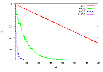
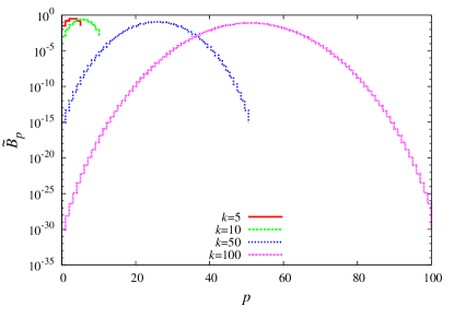
To complete the definition of the model, it has to be specified how the elements of the neighborhoods are chosen. In the most commonly used versions of the model, the $k$ interacting loci are either picked at random or taken to be adjacent along the sequence [28, 29]. A third possibility is to subdivide the sequence into blocks of size $k$, such that within blocks every locus interacts with every other but blocks are mutually independent [42, 43]. Although the construction of the neighborhoods affects certain properties of the landscapes such as the number of local fitness maxima [44, 45] and the evolutionary accessibility of the global maximum [21, 46], it turns out that the autocorrelation function does not depend on it. The autocorrelation function of the $NK$-model can be calculated starting from eq. (12) and is given by [47]

$$R_{d}=\binom{N-k}{d}\binom{N}{d}^{-1},$$ (21)

see fig. 2. Note that previously some incorrect expressions for the correlation functions have been reported in the literature [48] which led to the erroneous conclusion that the choice of the neighborhood affects the amplitude spectra [31].

Inserting (21) into eq. (18) yields

$$\tilde{B}_{q}=2^{-N}\sum_{d\geq 0}K^{(2)}_{q}(d)\binom{N-k}{d}.$$ (22)

The evaluation of this expression is somewhat technical and can be found in Appendix A. The final result

$$\tilde{B}_{q}=2^{-k}\binom{k}{q}$$ (23)

is remarkably simple (see fig. 2 for illustration). As expected, the Fourier coefficients vanish for $q>k$ [21, 49] and the known case of the HoC-model is reproduced for $k=N$. Moreover, the coefficients satisfy the symmetry $\tilde{B}_{q}=\tilde{B}_{k-q}$ and are maximal for $q=k/2$, as was previously conjectured in [31].

The $NK$-model is already a very flexible model and offers many possibilities for tuning. An even more general model is obtained by considering superpositions of $NK$-models, in the sense of $NK$-fitness landscapes being added independently. Let $\{F_{m}(\sigma)=\frac{1}{\sqrt{N}}\sum_{j}f^{(m)}_{j}(\sigma_{j_{1}},\dots,\sigma_{j_{k^{(m)}}})\}$ be a family of $n$ $NK$-fitness landscapes with neighborhood sizes $k^{(m)}$, $m=1,...,n$. Then its superposition $\mathcal{F}$ is defined by

$$\mathcal{F}:\sigma \mapsto\sum_{m=1}^{n}F_{m}(\sigma)$$

$$=\sum_{m=1}^{n}\frac{1}{\sqrt{N}}\sum_{j=1}^{N}f^{(m)}_{j}(\sigma_{j_{1}},\dots,\sigma_{j_{k^{(m)}}}).$$ (24)

Since the different $NK$-landscapes $\{F_{m}\}$ are independent, the correlation functions are additive,

$$R^{\mathcal{F}}_{d}=\frac{\sum_{m=1}^{n}\binom{N-k^{(m)}}{d}\binom{N}{d}^{-1}D_{m}}{\sum_{j=1}^{n}D_{j}}=:\sum_{i=0}^{N}A_{i}\binom{N-i}{d}\binom{N}{d}^{-1},$$ (25)

with statistical weights

$$A_{i}=\sum_{\{m|k^{(m)}=i\}}\frac{D_{m}}{\sum_{j=1}^{n}D_{j}},$$

where $D_{m}=\mathrm{Var}(f^{(m)})$. The sum is over all landscapes with neighborhoods of size $i$ and contains a zeroth order term that shifts the correlation function by a constant. The amplitude spectrum of the superposition is thus of the form

$$\tilde{B}^{\mathcal{F}}_{p}=\sum_{i\geq 0}2^{-i}A_{i}\binom{i}{p}.$$ (26)

Note that the consistent interpretation of an empirical fitness landscape as a superposition of $NK$-landscapes requires all $A_{i}$ to be positive. Nevertheless, it can be useful to consider superpositions containing negative $A_{i}$ to calculate amplitude spectra of fitness landscapes constructed by different means (see section 4 for an example).

Interestingly, expression (26) is also obtained from another type of generalized $NK$-model, giving rise to a different biological interpretation of the decomposition. Consider again fitness values $F(\sigma)$ that are constructed as sums of fitnesses corresponding to HoC-landscapes associated to $NK$-like neighborhoods $f_{i}(\sigma_{i_{1}},\dots,\sigma_{i_{k^{(i)}}})$,

$$F:\sigma\mapsto\sum_{i=1}^{M}f_{i}(\sigma_{i_{1}},\dots,\sigma_{i_{k^{(i)}}}),$$ (27)

where $M$ is an integer that can be different from $N$, and $k^{(i)}$ is the size of the $i$–th neighborhood, drawn from some distribution $P(k)$. Furthermore, for simplicity assume that the variances $D_{i}$ of the $f_{i}$ are all the same. The reasoning behind this model is to retain the idea of interacting groups of loci that is inherent in the $NK$-model, but to relax the rather unrealistic condition that all these groups are of the same size. Rather, it is assumed that there exist some typical distribution for the sizes of the groups.

Following the procedure explained in [47], the corresponding autocorrelation function is easily shown to be

$$R^{P}_{d}=\sum_{k\geq 0}P(k)\binom{N-k}{d}\binom{N}{d}^{-1},$$ (28)

which trivially leads to expression (26) with $A_{k}=P(k)$. The coefficients obtained from the decomposition of experimentally obtained spectra in terms of $NK$-spectra could therefore also be interpreted as a probability distribution for the sizes of interacting neighborhoods. Again, this interpretation is only consistent if all weights are positive. Here, it seems reasonable to expect that for large enough landscapes $P(k)$ should become continuous in the sense that the distribution becomes monotonic over large contiguous parts of its support.

4 Rough Mount Fuji model

Another model with tunable epistatic effects is the Rough Mount Fuji (RMF) model [30], which is constructed by superimposing a purely additive model and a HoC-landscape according to

$$F:\sigma\mapsto f_{0}+\sum_{i=1}^{N}b_{i}\sigma_{i}+\xi(\sigma).$$ (29)

In ref. [30], $f_{0}$ and the $b_{i}$ were parameters to be determined empirically from experimental data. Here we instead choose $f_{0}$ as some arbitrary constant, the $b_{i}$ as $N$ i.i.d. random variables, and $\xi(\sigma)$ as another set of $2^{N}$ i.i.d. random variables with $\langle\xi(\sigma)\rangle=0$ and $\langle\xi(\sigma)\xi({\sigma^{\prime}})\rangle=D_{N}\delta_{\sigma\sigma^{\prime}}$, compare to the construction of the HoC-model above in sect. 3. Note that, in contrast to the $\xi$, the $b_{i}$ do not depend on $\sigma$. The amount of ruggedness is controlled by fixing the variance of the HoC-component, $D_{N}$, and the mean of the absolute values of the slopes of the additive model, $s=\sum_{i=1}^{N}|b_{i}|/N$. The important limiting cases, the HoC-model and the purely additive model, are obtained in the limits $D_{N}/s\rightarrow\infty$ and $D_{N}/s\rightarrow 0$, respectively [17].

Figure 3: The autocorrelation function (top) and the amplitude spectrum (bottom) for the RMF-model with $N=100$, $D_{1}=0$, $D_{N}=1$ and various values of $c$.

In the following we write $b_{i}=\frac{c}{2}+\zeta_{i}$, where $c$ is a constant independent of $i$, and the $\zeta_{i}$ are i.i.d. random variables with $\langle\zeta_{i}\rangle=0$ and $\langle\zeta_{i}\zeta_{j}\rangle=D_{1}\delta_{ij}$. Note that choosing the same mean value for all the $b_{i}$’s singles out the reference sequence $\sigma^{(0)}=(1,\ldots,1)$. On average, the fitness of sequence $\sigma$ decays linearly with the Hamming distance $d(\sigma,\sigma^{(0)})$ to the reference sequence $\sigma^{(0)}$ and the mean slope is $c$. Setting $D_{1}=0$ yields a simpler version of the RMF-model that was introduced in [20].

To calculate the autocorrelation function of the RMF-model, it is convenient to rewrite the fitness as $F(\sigma)=\alpha-cd(\sigma,\sigma^{(0)})+\sum_{i=1}^{N}\zeta_{i}\sigma_{i}+\xi(\sigma)$, where $\alpha=f_{0}+\frac{Nc}{2}$. Making use of the vanishing mean values of the $\zeta_{i}$’s and the $\xi$’s, the autocorrelation function reads

$$R_{d}= \Bigg{(}\left\langle\sum_{i=1}^{N}\zeta_{i}\sigma_{i}\sum_{j=1}^{N}\zeta_{j}\sigma^{\prime}_{j}\right\rangle_{d}+\langle\xi(\sigma)\xi(\sigma^{\prime})\rangle_{d}$$

$$+\langle(\alpha-cd(\sigma,\sigma^{(0)}))(\alpha-cd(\sigma^{\prime},\sigma^{(0)}))\rangle_{d}$$

$$-\left(\overline{\alpha-cd(\sigma,\sigma^{(0)})}\right)^{2}\Bigg{)}\cdot$$

$$\Bigg{(}\overline{(\alpha-cd(\sigma,\sigma^{(0)}))^{2}}-\left(\overline{\alpha-cd(\sigma,\sigma^{(0)})}\right)^{2}$$

$$+\left\langle\Bigg{(}\sum_{i=1}^{N}\zeta_{i}\sigma_{i}\Bigg{)}^{2}\right\rangle+\left\langle\xi(\sigma)^{2}\right\rangle\Bigg{)}^{-1}.$$

The covariance of the deterministic part has been evaluated elsewhere and the terms containing random variables can easily be calculated, yielding

$$R^{\mathrm{RMF}}_{d}=\frac{\left(D_{1}+\frac{c^{2}}{4}\right)(N-2d)+D_{N}\delta_{d0}}{\left(D_{1}+\frac{c^{2}}{4}\right)N+D_{N}}.$$

In order to obtain the spectrum $\tilde{B}_{p}$ we write $R^{\mathrm{RMF}}_{d}$ as a linear combination of correlation functions of the $NK$-model with different $k$’s, i.e. $R^{\mathrm{RMF}}_{d}=\sum_{k=0}^{N}A_{k}\binom{N-k}{d}/\binom{N}{d}$ with expansion coefficients

$$A_{0} =-\frac{\left(D_{1}+\frac{c^{2}}{4}\right)N}{\left(D_{1}+\frac{c^{2}}{4}\right)N+D_{N}},\;A_{1}=\frac{2\left(D_{1}+\frac{c^{2}}{4}\right)N}{\left(D_{1}+\frac{c^{2}}{4}\right)N+D_{N}},$$

$$A_{N} =\frac{D_{N}}{\left(D_{1}+\frac{c^{2}}{4}\right)N+D_{N}},$$ (30)

and $A_{k}=0$ for all other $k$’s. The $\tilde{B}_{p}$ can now be calculated making use of the linearity of equation (18), yielding

$$\tilde{B}^{\mathrm{RMF}}_{p}=\frac{\left(D_{1}+\frac{c^{2}}{4}\right)N\delta_{p1}+D_{N}2^{-N}\binom{N}{p}}{\left(D_{1}+\frac{c^{2}}{4}\right)N+D_{N}}.$$ (31)

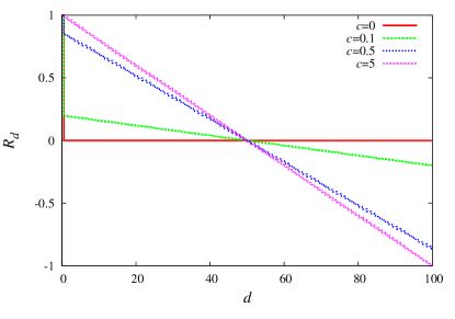
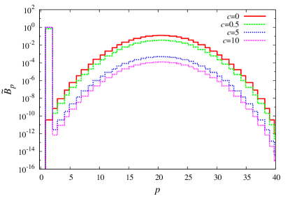
In fig. 3, autocorrelation functions and amplitude spectra for the RMF-model with $D_{1}=0$ and various choices of $c$ are shown. Note that the generality of the superposition ansatz made it possible to calculate the $\tilde{B}_{p}$ for the RMF-model, although the relation to the $NK$-model is not obvious at first sight. Having in mind that the zeroth component does not contain information about epistasis, we adopt, for the rest of this paper, a more general definition of RMF-landscapes as superpositions of $NK$ -landscapes with all components being equal to zero, except for $A_{1}>0$, $A_{N}>0$, and an arbitrary zeroth order coefficient $A_{0}$ that may be of any sign.

5 Exponentially decaying correlation functions

Figure 4: The amplitude spectrum $\tilde{B}_{p}$ (main) and the renormalized spectrum $\tilde{\beta}_{p}$ (inset) for exponentially decaying fitness correlations. In the inset, the exponential decay is obvious.

The motivation for the present paper is to identify typical features of amplitude spectra of fitness landscapes and to make use of them for extracting information about the underlying biological system. In the preceding two sections we considered well-established statistical models of fitness landscapes and computed their spectra. As will be further illustrated in sect. 6, this analysis provides criteria to judge whether a measured spectrum can be explained by these models or not and, if so, one can use the biological picture behind the model to try to interpret the findings.

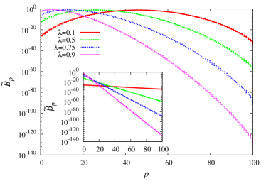
However, when faced with experimental data, none of the presented models may be general enough to give a good description. If this is the case, an alternative ansatz is to start with a presumably generic correlation function and calculate the corresponding spectrum, which can be compared to the data. This may then also guide the search for improved models. Here, we consider a correlation function that decays exponentially with Hamming distance $d$

$$R^{\mathrm{exp}}_{d}=\lambda^{d},$$ (32)

with $0<\lambda<1$. The resulting expression for the spectrum obtained from eq. (18),

$$\tilde{B}_{q}=2^{-N}\sum_{d\geq 0}\binom{N}{d}K^{(2)}_{q}(d)\lambda^{d},$$ (33)

is most easily evaluated using the known form of the generating function of the Krawtchouk polynomials [35, 36]

$${\cal K}^{(2)}(x,z)=\sum_{n\geq 0}K^{(2)}_{n}(x)\,z^{n}=(1-z)^{x}(1+z)^{N-x}$$ (34)

and the fact that these polynomials are self-dual in the sense of [50]

$$\binom{N}{x}K^{(2)}_{n}(x)=\binom{N}{n}K^{(2)}_{x}(n).$$ (35)

Indeed, inserting (35) into (33) and using (34) yields

$$\tilde{B}_{q}=2^{-N}\binom{N}{q}(1-\lambda)^{q}(1+\lambda)^{N-q}.$$ (36)

Defining $\kappa=\ln{\left(\frac{1+\lambda}{1-\lambda}\right)}$ this expression can be rewritten as

$$\tilde{B}_{q}=\frac{\binom{N}{q}}{(1+\mathrm{e}^{-\kappa})^{N}}\mathrm{e}^{-\kappa q},$$ (37)

corresponding to $R^{\mathrm{exp}}_{d}=\left(1-\frac{2}{1+\mathrm{e}^{\kappa}}\right)^{d}$. We conclude that if the spectrum normalized with respect to the number of $q$–tuples, $\tilde{\beta}_{q}=\tilde{B}_{q}/\binom{N}{q}$, decays exponentially with $q$, then the correlations decay exponentially with distance on the hypercube, see fig. 4.

Although we are, at the moment, lacking simple stochastic models that produce exponentially decaying correlations, spectra of the form (37) have recently been found for fitness landscapes obtained from a dynamical model of molecular signal transduction [51]. It would be interesting to see whether one can construct stochastic models that do not enter too deeply into the dynamics at the cellular level but contain a simple and generic mechanism that gives rise to such correlations.

Exponentially decaying correlations have also been reported in a recent large-scale study of the fitness landscape of HIV-1 [52]. However, the correlation function calculated in that article is different from the one studied here, as it averages over correlations between fitness values of mutants that are connected by random walks of some length $s$ and not over fitness values corresponding to states separated by Hamming distance $d$. Such random walk correlation functions are also connected in a simple manner to the amplitude spectra [34], but the relation is different from the one considered here. Therefore our results are not directly applicable to these observations.

6 Experimentally obtained fitness landscapes

Figure 5: Spectra corresponding to various experimentally measures fitness landscapes. The green lines are obtained by fitting the spectrum of a superposition of $NK$-models to the data. The dashed red line is proportional to $\binom{N}{p}$, showing the spectrum expected for a HoC-component.

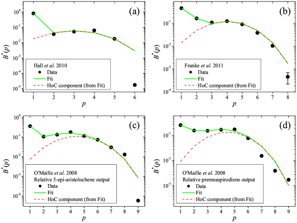
In this section we compare the model spectra to several experimentally measured “fitness” landscapes. The quotation marks indicate that not all of the landscapes presented here actually correspond to fitness, but rather to some proxy of it. To be able to compare spectra, the landscapes should be as large and as complete as possible. The four landscapes considered are a six locus landscapes obtained by Hall et al. [11] for the yeast Saccharomyces cerevisiae, an eight locus landscape for the fungus Aspergillus niger presented by Franke et al. [20], and two nine locus landscapes for the plant Nicotiana tabacum studied by O’Maille et al. [8]. A comparative analysis of these (and other) empirical landscapes can be found in [17]. All spectra presented in this section were calculated directly by decomposing the fitness landscapes in terms of the eigenfunctions of the graph Laplacian.

While the first two landscapes mentioned above measure growth rate as a quantifier of fitness, the landscapes presented in [8] measure enzymatic specificity of terpene synthases, that is, the relative production of 5-epi-aristolochene and premnaspirodiene, respectively. As for these landscapes only 418 out of 512 fitness values were measured, the missing data is estimated by fitting a multidimensional linear model [53] to the measured landscape. The fitness values of states for which there are no measurements are then replaced by the values given by the linear model. On the contrary, for the A. niger landscape considered in [20], missing fitness values were argued to correspond to non-viable mutants and are therefore set to zero. The way of estimating missing values obviously affects the spectra, but some estimation is necessary to be able to carry out the analysis.

We now ask whether the experimental spectra can be expressed as superpositions of $NK$-spectra of the form (26) (recall that the RMF-model is a particular case of such a superposition). Of course, such a decomposition is always possible, but the assumption that the biological mechanism responsible for the spectra is really the additive interplay of fixed groups of loci of characteristic sizes is only reasonable if all the coefficients $A_{j}$ are positive.

Simply solving the linear system of equations (26) generally yields several negative coefficients. More satisfactory results are obtained by fitting a function of the form (26) to the data by means of a least square procedure, constraining the coefficients to positive values. Here, two ansatzes are considered. First a fit containing all coefficients is carried out, with none of the $A_{j}$ fixed to zero a priori. This is done to check whether a superposition of type (28) with a continuous neighborhood size distribution $P(k)$ is appropriate. Second, sparse fits containing as few nonzero $A_{j}$’s as possible are carried out to verify if the landscape could be biologically interpreted as a superposition of a small number of $NK$-landscapes of different interaction ranges. One way of selecting $A_{j}$’s that can be neglected in the fit is to identify those coefficients obtained in the full fit that are much smaller than the others. In all cases, the term proportional to $A_{0}$ in (26) is not considered as it can always be trivially fixed to fit $\tilde{B}_{0}$.

In fig. 5 the data for the normalized amplitudes $B_{p}^{\ast}$ (black dots) is shown together with the fit (green curve) and the HoC-component $\sim\binom{N}{p}$ (red dashed line) of the fit. For the A. niger landscape in [20] error estimates for the fitness values were available [54], enabling the calculation of error bars to the spectrum. This is done by constructing ensembles of landscapes with fitness values $F(\sigma)=\langle F(\sigma)\rangle+\xi(\sigma)$, where $\langle F(\sigma)\rangle$ is the mean of the replicate experimental measurements of the fitness of genotype $\sigma$ and the $\xi(\sigma)$ are normally distributed random numbers with $\sigma$-dependent standard deviations obtained from the replicate measurements. Note that the influence of the measurement errors on the spectra is very small and only exceeds the symbol size for the highest $p$ component ($p=8$). At least for this case one can therefore safely exclude that the HoC-component of the spectrum is generated by measurement errors.

As can be seen in fig. 5(a), the spectrum of the yeast landscape [11] is nicely fitted by an ansatz where only $A_{1}$ and $A_{N}$ are assumed to be different from zero. This is evidently a superposition of an additive and a HoC-landscape and therefore a RMF-landscape. Only the value at $p=N$ seems too small to be fitted by the model. However, this value corresponds to a single component of the decomposition (5) and the large deviation may be due to the lack of averaging. Also for the A. niger landscape from [20] a nice and sparse fit with nonzero coefficients $A_{1}$, $A_{2}$, and $A_{N}$ is obtained (see Fig. 5(b)). The significant value of $A_{2}$ implies that there are important interactions between pairs of loci. A RMF -landscape is therefore not an appropriate model of this system. Note that this conclusion differs from the analysis presented in [20], where a reasonable fit to the RMF-model was found for a particular epistasis measure, the number of accessible pathways. This illustrates the importance of using more than one topographic measure for the comparison between empirical and model landscapes [17].

For the spectrum of the 5-epi-aristolochene N. tabacum landscape from [8], the fitting yields reasonable results for an ansatz allowing only $A_{1}$, $A_{2}$, $A_{6}$ and $A_{N}$ to be different from 0 (see Fig. 5(c)). This might indicate that, apart from the non epistatic part and the simple pair interactions, there are one or several groups consisting of six strongly interacting alleles. Using the same ansatz for the premnaspirodiene landscape yields less convincing results, as the large $p$ part of the spectrum seems to be poorly fitted (see Fig. 5(d)). Introducing more components into the fitting ansatz yields better results for this part of the spectrum, but such ansatzes can hardly be considered sparse anymore.

Using the full ansatz to fit the different landscapes does not yield any qualitative improvement for the first three landscapes and provides no evidence for an underlying continuous neighborhood size distribution $P(k)$. Only for the premnaspirodiene N. tabacum landscape does the fit for the spectrum improve notably, but the obtained spectrum does not support the idea of a continuous distribution of neighborhood sizes (not shown). In general, such a continuous distribution is more likely to emerge for larger landscapes than the relatively small data sets considered here, which suffer from insufficient averaging over groups of loci of different sizes.

One should be aware that failing to obtain a reasonable decomposition of an empirical landscape in terms of $NK$-spectra does not a priori rule out the possibility that the landscape is in fact shaped by the mechanisms assumed by a superposition of $NK$-models. For example, the failure may be due to an inappropriate fitness measure, in the following sense. Suppose that there exists a fitness proxy, $F^{\prime}(\sigma)$, whose decomposition in terms of $NK$-landscapes is sparse, but the proxy actually measured in experiments is $F=G(F^{\prime})$, with $G$ being some nonlinear function. The decomposition of $F$ may then not be sparse anymore and the biological mechanism that shapes the landscape may be obscured.

Finally, it was checked whether any of the spectra are compatible with the expression (37) corresponding to an exponentially decaying correlation function, but no reasonable correspondence was found. Of course, this does not allow for the conclusion that exponentially decaying correlations are an unrealistic assumption. Possibly, it may again be necessary to go to larger landscape sizes to see such behavior. Also, the way in which the mutations constituting the landscape are selected may have an influence on the observed correlations (see e.g. [17]).

7 Conclusions

Exploiting the connection between amplitude spectra and fitness autocorrelation functions of fitness landscapes over the Boolean hypercube, the amplitude spectrum of Kauffman’s $NK$-model was calculated exactly and found to be of the simple form (23). By superimposing $NK$-landscapes the spectra of RMF-type models could also be obtained. In addition, an $NK$-like model with a distribution $P(k)$ of neighborhood sizes was introduced and its spectrum was calculated. Such an extension of the $NK$-model is reasonable, because it cannot be assumed in general that every locus interacts with the same number of other loci. This model thus offers more flexibility to fit experimental data. As a last example, the spectrum of a model with exponentially decaying correlations was computed.

The HoC, RMF and $NK$-models are frequently used for analyzing evolutionary processes, classifying fitness landscape properties and fitting experimental data. Therefore a lot of effort has been invested in the understanding of these models, but the link to experimental data is still rather weak. The amplitude spectra calculated in this article should facilitate quantitative comparisons in future studies. The spectra contain a large amount of information about the landscape topography, and it is important to understand how the spectrum encrypts this information in order to be able to interpret the spectra of measured fitness landscapes. As an exemplary application of our results, four experimental landscapes were fitted by means of the model spectra. Three of them could be fitted very nicely with sparse superpositions of $NK$-models, while for the fourth one the obtained fit seems less convincing. In none of the cases evidence for a continuous neighborhood size distribution $P(k)$ was found, which might be due to the small sizes of the landscapes discussed in this article.

We claim that the fitting of amplitude spectra can be a useful tool for data analysis, but it has to be emphasized that the spectra cannot be assigned to model landscapes in a unique way. Also, the collection of models presented here is by no means exhaustive. Obtaining analytical expressions for the amplitude spectra of other classes of fitness landscapes is desirable and should prove helpful in guiding the search for suitable models of experimental landscapes.

Finally, it is important to mention that there are interesting and biologically relevant properties of fitness landscapes that cannot be obtained from their spectra, such as, for example, the number of local fitness maxima and the number of selectively accessible pathways [6, 20]. While it was shown in ref. [17] that the ruggedness measure $B_{\mathrm{sum}}$ based on the Fourier decomposition correlates with both quantities, there is no strict correspondence between these measures of epistatic interactions. Amplitude spectra do not distinguish between different kinds of epistasis, i.e. magnitude, sign, or reciprocal sign epistasis, in a qualitative way. Therefore, if one is interested in this distinction, other epistasis measures have to be included in the analysis.

Appendix A Fourier spectrum of the $NK$-model

To evaluate the expression (22), an alternative but equivalent formulation for the Krawtchouk polynomials is needed. With [36]

$$K^{(2)}_{q}(d)=\sum_{i\geq 0}(-2)^{i}\binom{d}{i}\binom{N-i}{q-i}$$

we obtain

$$\tilde{B}_{q} =\sum_{d\geq 0}K^{(2)}_{q}(d)\binom{N-k}{d}$$

$$=2^{-N}\sum_{i\geq 0}\sum_{d\geq 0}(-2)^{i}\binom{d}{i}\binom{N-i}{q-i}\binom{N-k}{d}.$$

The summation over $d$ can be carried out using the identity [55]

$$\sum_{d\geq 0}\binom{d}{i}\binom{N-k}{d}=2^{N-k-i}\binom{N-k}{i},$$

which yields

$$\tilde{B}_{q}=2^{-k}\sum_{i\geq 0}(-1)^{i}\binom{N-i}{q-i}\binom{N-k}{i}.$$ (38)

At this point we relax the condition (15) of positivity on the entries of the binomial coefficients. This allows us to perform an ‘upper negation’ [56] in the first binomial factors in eq.(38),

$$\binom{N-i}{q-i}=(-1)^{q-i}\binom{q-N-1}{q-i}.$$

The remaining sum over $i$ can now be evaluated using the Vandermonde identity [56],

$$\tilde{B}_{q} =2^{-k}(-1)^{q}\sum_{i\geq 0}\binom{q-N-1}{q-i}\binom{N-k}{i}$$

$$=2^{-k}(-1)^{q}\binom{q-k-1}{q}$$

and with another upper negation we arrive at the final result (23).

References

- Wright [1932] Wright, S. (1932). The roles of mutation, inbreeding, crossbreeding and selection in evolution. Proc. of the 6th Int. Cong. of Genetics 1, 356–366.
- Binder & Young [1986] Binder, K. & Young, A.P. (1986). Spin glasses: Experimental facts, theoretical concepts, and open questions. Rev. Mod. Phys. 58, 801 – 976.
- Mézard et al. [1987] Mézard, M., Parisi, G. & Virasoro, M. (1987). Spin Glass Theory and Beyond. Singapore: World Scientific.
- Garey & Johnson [1979] Garey, M. & Johnson, D. (1979). Computers and Intractability. A Guide to the Theory of Completeness. San Francisco: Freeman.
- Lunzer et al. [2005] Lunzer, M., Miller, S.P., Felsheim, R. & Dean, A.M. (2005). The biochemical architecture of an ancient adaptive landscape. Science 310, 499–501.
- Weinreich et al. [2006] Weinreich, D.M., Delaney, N.F., DePristo, M.A. & Hartl, D.L. (2006). Darwinian evolution can follow only very few mutational paths to fitter proteins. Science 312, 111–114.
- Poelwijk et al. [2007] Poelwijk, F.J., Kiviet, D.J., Weinreich, D.M. & Tans, S.J. (2007). Empirical fitness landscapes reveal accessible evolutionary paths. Nature 445, 383–386.
- O’Maille et al. [2008] O’Maille, P.E., Malone, A., Dellas, N., Hess Jr, B.A., Smentek, L., Sheehan, I., Greenhagen, B.T. & et al. (2008). Quantitative exploration of the catalytic landscape separating divergent plant sesquiterpene synthases. Nat. Chem. Biol. 4, 617–623.
- Lozovsky et al. [2009] Lozovsky, E.R., Chookajorn, T., Browna, K.M., Imwong, M., Shaw, P.J., Kamchonwongpaisan, S., Neafsey, D.E. & et al. (2009). Stepwise acquisition of pyrimethamine resistance in the malaria parasite. Proc. Natl. Acad. Sci. USA 106, 12025–12030.
- Brown et al. [2010] Brown, K.M., Costanzo, M.S., Xu, W., Roy, S., Lozovsky, E.R. & Hartl, D.L. (2010). Compensatory mutations restore fitness during the evolution of dihydrofolate reductase. Mol. Biol. Evol. 27, 2682–2690.
- Hall et al. [2010] Hall, D.W., Agan, M., & Pope, S.C. (2010). Fitness epistasis among six biosynthetic loci in the budding yeast Saccharomyces cerevisiae. J. Hered. 101, S75–S84.
- da Silva et al. [2010] da Silva, J., Coetzer, M., Nedellec, R., Pastore, C. & Mosier, D.E. (2010). Fitness epistasis and constraints on adaptation in a human immunodeficiency virus type 1 protein region. Genetics 185, 293–303.
- Costanzo et al. [2011] Costanzo, M.S., Brown, K.M. & Hartl, D.L. (2011). Fitness trade-offs in the evolution of dihydrofolate reductase and drug resistance in Plasmodium falciparum. PLoS ONE 6, e19636.
- Chou et al. [2011] Chou, H.-H., Chiu, H.-C., Delaney, N.F., Segrè, D., & Marx, C.J. (2011). Diminishing returns epistasis among beneficial mutations decelerates adaptation. Science 332, 1190–1192.
- Khan et al. [2011] Khan, A.I., Dinh, D.M., Schneider, D., Lenski, R.E. & Cooper, T.F. (2011). Negative epistasis between beneficial mutations in an evolving bacterial population. Science 332, 1193–1196.
- Tan et al. [2011] Tan, L., Serene, S., Chao, H.X. & Gore, J. (2011). Hidden randomness between fitness landscapes limits reverse evolution. Phys. Rev. Lett. 106, 198102.
- Szendro et al. [2012] Szendro, I.G., Schenk, M.F., Franke, J., Krug, J. & de Visser, J.A.G.M. (2013). Quantitative analyses of empirical fitness landscapes. J. Stat. Mech. Theor. Exp. P01005.
- de Visser et al. [2011] de Visser, J.A.G.M., Cooper, T.F. & Elena, S.F. (2011). The causes of epistasis. Proc. R. Soc. London B 278, 3617–3624.
- Weinreich et al. [2005] Weinreich, D.M., Watson, R.A. & Chao, L. (2005). Perspective: Sign epistasis and genetic constraint on evolutionary trajectories. Evolution 59, 1165–1174.
- Franke et al. [2011] Franke, J., Klözer, A., de Visser, J.A.G.M. & Krug, J. (2011). Evolutionary accessibility of mutational pathways. PLoS Comput Biol 7(8), e1002134.
- Franke & Krug [2012] Franke, J. & Krug, J. (2012). Evolutionary accessibility in tunably rugged fitness landscapes. J. Stat. Phys. 148, 705–722.
- Orr [2002] Orr, H.A. (2002). The population genetics of adaptation: the adaptation of DNA sequences. Evolution 56(7), 1317–1330.
- Joyce et al. [2008] Joyce, P., Rokyta, D.R., Beisel, C.J. & Orr, H.A. (2008). A general extreme value theory model for the adaptation of DNA sequences under strong selection and weak mutation. Genetics 180, 1627–1643.
- Poelwijk et al. [2010] Poelwijk, F.J., Tănase-Nicola, S., Kiviet, D.J. & Tans, S.J. (2010). Reciprocal sign epistasis is a necessary condition for multi-peaked fitness landscapes. J. Theor. Biol. 272, 141–144.
- Neidhart & Krug [2011] Neidhart, J. & Krug, J. (2011). Adaptive walks and extreme value theory. Physical Review Letters 107, 178102.
- Crona et al. [2013] Crona, K., Greene, D. & Barlow, M. (2013). The peaks and geometry of fitness landscapes. J. Theor. Biol. 317, 1–10.
- Weinberger [1991] Weinberger, E.D. (1991). Fourier and Taylor series on fitness landscapes. Biol. Cybern. 65, 321–330.
- Kauffman & Weinberger [1989] Kauffman, S.A. & Weinberger, E.D. (1989). The NK model of rugged fitness landscapes and its application to maturation of the immune response. Journal of Theoretical Biology 141(2), 211–245.
- Kauffman [1993] Kauffman, S.A. (1993). The Origins of Order: Self-Organization and Selection in Evolution. Oxford University Press, USA.
- Aita et al. [2000] Aita, T., Uchiyama, H., Inaoka, T., Nakajima, M., Kokubo, T. & Husimi, Y. (2000). Analysis of a local fitness landscape with a model of the rough Mt. Fuji-type landscape: application to prolyl endopeptidase and thermolysin. Biopolymers 54, 64–79.
- Stadler & Happel [1999] Stadler, P.F. & Happel, R. (1999). Random field models for fitness landscapes. J. Math. Biol. 38, 435–478.
- Maynard Smith [1970] Maynard Smith, J. (1970). Natural selection and the concept of a protein space. Nature 225, 563–564.
- Neher & Shraiman [2011] Neher, R.A & Shraiman, B.I. (2011). Statistical genetics and evolution of quantitative traits. Rev. Mod. Phys. 83, 1283–1300.
- Stadler [1996] Stadler, P.F. (1996). Landscapes and their correlation functions. J. Math. Chem. 20, 1–45.
- Szegö [1994] Szegö, G. (1975). Orthogonal polynomials. American Mathematical Society Colloquium Publications, vol. 23, 4th edition, Providence, R.I., 1975.
- Stoll [2011] Stoll, T. (2011). Reconstruction Problems for Graphs, Krawtchouk Polynomials, and Diophantine Equations. In Structural Analysis of Complex Networks, ed. by M. Dehmer (Birkhäuser, Boston) pp. 293–317.
- Kingman [1978] Kingman, J.F.C. (1978). A simple model for the balance between selection and mutation. J. Appl. Prob. 15, 1–12.
- Kauffman & Levin [1987] Kauffman, S. & Levin, S. (1987). Towards a general theory of adaptive walks on rugged landscapes. J. Theor. Biol 128, 11–45.
- Miller et al. [2011] Miller, C.R., Joyce, P. & Wichman, H.A. (2011). Mutational Effects and Population Dynamics During Viral Adaptation Challenge Current Models. Genetics 187, 185–202.
- Welch & Waxman [2005] Welch, J.J. & Waxman, D. (2005). The nk model and population genetics. J. Theor. Biol. 234, 329–340.
- Altenberg [1997] Altenberg, L. (1997). NK fitness landscapes. In Handbook of Evolutionary Computation, ed. by T. Bäck, D.B. Fogel and Z. Michalewicz (IOP Publishing Ltd and Oxford University Press).
- Perelson & Macken [1995] Perelson, A.S. & Macken, C.A. (1995). Protein evolution on partially correlated landscapes. Proceedings of the National Academy of Sciences 92(21), 9657–9661.
- Orr [2006] Orr, H.A. (2006). The population genetics of adaptation on correlated fitness landscapes: The block model. Evolution 60(6), 1113–1124
- Weinberger [1991a] Weinberger, E.D. (1991). Local properties of Kauffman’s N-k model: A tunably rugged energy landscape. Phys. Rev. A 44, 6399–6413.
- Limic & Pemantle [2004] Limic, V. & Pemantle, R. (2004). More rigorous results on the Kauffman-Levin model of evolution. Annals of Probability 32, 2149–2178.
- Schmiegelt [2012] Schmiegelt, B. (2012). Bachelor thesis, University of Cologne.
- Campos et al. [2002] Campos, P.R.A., Adami, C. & Wilke, C.O. (2002). Optimal adaptive performance and delocalization in NK fitness landscapes. Physica A 304, 495–506; ibid. 318, 637 (Erratum).
- Fontana et al. [1993] Fontana, W., Stadler, P.F., Bornberg-Bauer, E.G., Griesmacher, T., Hofacker, I.L., Tacker, M., Tarazona, P., Weinberger, E.D. & Schuster, P. (1993). RNA folding and combinatory landscapes. Phys. Rev. E 47, 2083–2099.
- Drossel [2001] Drossel, B.(2001). Biological evolution and statistical physics Adv. Phys. 50, 209–295.
- Koekoek eg al. [2010] Koekoek, R., Lesky, P. A. & Swarttouw, R. F. (2010) Hypergeometric Orthogonal Polynomials and Their q-Analogues. Springer Monographs in Mathematics.
- Pumir & Shraiman [2011] Pumir, A. & Shraiman, B. (2011). Epistasis in a model of molecular signal transduction. PLoS Comput. Biol. 7, e1001134.
- Kouyos et al. [2012] Kouyos, R.D., Leventhal, G.E., Hinkley, T., Haddad, M., Whitcomb, J.M., Petropoulos, C.J. & Bonhoeffer, S. (2012). Exploring the complexity of the HIV-1 fitness landscape. PLoS Genet. 8(93), e1002551.
- Aita et al. [2001] Aita, T., Iwakura, M. & Husimi, Y. (2001). A cross-section of the fitness landscape of dihydrofolate reductase. Protein Eng. 14, 633–638.
- Franke [2012] Franke, J. (2012). Statistical topography of fitness landscapes. Doctoral thesis, University of Cologne.
- Gould [2010] Gould, H. W. (2010). Tables of Combinatorial Identities Vol.2, ed. by J. Quaintance. Available online at www.math.wvu.edu/gould/.
- Graham et al. [1994] Graham, R. L., Knuth, D. E. & Patashnik, O. (1994). Concrete Mathematics. Addison-Wesley Publishing Company, 2 ed.