CFHTLenS: Higher-order galaxy-mass correlations probed by galaxy-galaxy-galaxy lensing

P. Simon1, T. Erben1, P. Schneider1, C. Heymans2, H. Hildebrandt3,1, H. Hoekstra4,5, T.D. Kitching2, Y. Mellier6, L. Miller7, L. Van Waerbeke3, C. Bonnett8, J. Coupon9, L. Fu10, M.J. Hudson11,12, K. Kuijken4, B.T.P. Rowe13,14, T. Schrabback1,4,15, E. Semboloni4, and M. Velander4,7
1Argelander Institute for Astronomy, University of Bonn, Auf dem Hügel 71, 53121 Bonn, Germany.
2Scottish Universities Physics Alliance, Institute for Astronomy,
  University of Edinburgh, Royal Observatory, Blackford Hill, Edinburgh, EH9 3HJ, UK.
3Department of Physics and Astronomy, University of British Columbia, 6224 Agricultural Road, Vancouver, V6T 1Z1, BC, Canada.
4Leiden Observatory, Leiden University, Niels Bohrweg 2, 2333 CA Leiden, The Netherlands.
5Department of Physics and Astronomy, University of Victoria, Victoria, BC V8P 5C2, Canada.
6Institut d’Astrophysique de Paris, Université Pierre et Marie Curie - Paris 6, 98 bis Boulevard Arago, F-75014 Paris, France.
7Department of Physics, Oxford University, Keble Road, Oxford OX1 3RH, UK.
8Institut de Ciencies de l’Espai, CSIC/IEEC, F. de Ciencies, Torre C5 par-2, Barcelona 08193, Spain.
9Institute of Astronomy and Astrophysics, Academia Sinica, P.O. Box 23-141, Taipei 10617, Taiwan.
10Key Lab for Astrophysics, Shanghai Normal University, 100 Guilin Road, 200234, Shanghai, China.
11Department of Physics and Astronomy, University of Waterloo, Waterloo, ON, N2L 3G1, Canada.
12Perimeter Institute for Theoretical Physics, 31 Caroline Street N, Waterloo, ON, N2L 1Y5, Canada.
13Department of Physics and Astronomy, University College London, Gower Street, London WC1E 6BT, UK.
14California Institute of Technology, 1200 E California Boulevard, Pasadena CA 91125, USA.
15Kavli Institute for Particle Astrophysics and Cosmology, Stanford University, 382 Via Pueblo Mall, Stanford, CA 94305-4060, USA
Email:psimon@astro.uni-bonn.de
(Version of )
Abstract

We present the first direct measurement of the galaxy-matter bispectrum as a function of galaxy luminosity, stellar mass and SED type. Our analysis uses a galaxy-galaxy-galaxy lensing technique (G3L), on angular scales between 9 arcsec to 50 arcmin, to quantify (i) the excess surface mass density around galaxy pairs (excess mass hereafter) and (ii) the excess shear-shear correlations around single galaxies, both of which yield a measure of two types of galaxy-matter bispectra. We apply our method to the state-of-the-art Canada-France-Hawaii Telescope Lensing Survey (CFHTLenS), spanning 154 square degrees. This survey allows us to detect a significant change of the bispectra with lens properties (stellar mass, luminosity and SED type). Measurements for lens populations with distinct redshift distributions become comparable by a newly devised normalisation technique. That will also aid future comparisons to other surveys or simulations. A significant dependence of the normalised G3L statistics on luminosity within 23Mr1823subscript𝑀𝑟18-23\leq M_{r}\leq-18 and stellar mass within 5×10⁹MM2×1011M5superscript109subscript𝑀direct-productsubscript𝑀2superscript1011subscript𝑀direct-product5\times 10^{9}M_{\odot}\leq M_{\ast}\leq 2\times 10^{11}M_{\odot} is found (h=0.730.73h=0.73). Both bispectra exhibit a stronger signal for more luminous lenses or those with higher stellar mass (up to a factor 2-3). This is accompanied by a steeper equilateral bispectrum for more luminous or higher stellar mass lenses for the excess mass. Importantly, we find the excess mass to be very sensitive to galaxy type as recently predicted with semi-analytic galaxy models: luminous (Mr<21subscript𝑀𝑟21M_{r}<-21) late-type galaxies show no detectable signal, while all excess mass detected for luminous galaxies seems to be associated with early-type galaxies. We also present the first observational constraints on third-order stochastic galaxy biasing parameters.

keywords:
dark matter - large-scale structure of Universe - gravitational lensing
pagerange: CFHTLenS: Higher-order galaxy-mass correlations probed by galaxy-galaxy-galaxy lensingDpubyear: 2008

1 Introduction

Over the course of the last two decades, the gravitational lensing effect has allowed us to establish a new branch of science that exploits the distortion of light bundles from distant galaxies (“sources”) in order to probe the large-scale gravitational field produced by intervening matter. Strong tidal gravitational fields cause an obvious distortion of individual galaxy images (“strong lensing”; cf. Meylan et al., 2006), whereas weak deflections can only be inferred by statistical methods utilising many galaxy images (“weak lensing”; cf. Schneider, 2006). For the latter, usually shear image distortions are harnessed, although the study of higher-order flexion distortions may also be feasible in the near future (cf. Goldberg & Natarajan, 2002; Goldberg & Bacon, 2005; Velander et al., 2011). Recently, the lensing magnification effect has also moved into the focus of research as new source of information on cosmological large-scale structure (Hildebrandt et al., 2009). As the gravitational field is solely determined by the mass density of the objects under examination, no further assumptions on their properties need to be made when studying lensing. This makes it a unique tool for cosmologists to examine the large-scale structure of the Universe, in particular the relation between luminous components, such as galaxies, and the dark component. Within the current ΛCDMΛCDM\Lambda\rm CDM standard model of cosmology (Peacock, 1999; Dodelson, 2003), the major fraction of matter is so-called dark matter, whereas ordinary baryonic matter is subdominant (Komatsu et al., 2011). Therefore, lensing plays a key role in scrutinising the dominant matter component or in testing the standard model.

Statistical methods have been developed that quantify the average mass distribution around galaxies by cross-correlating tangential shear, as observed from background sources, with foreground lens galaxy positions. Galaxy-galaxy lensing (GGL), as the first highly successful application, in effect measures the stacked projected surface mass density profiles around galaxies (Brainerd et al., 1996; Hudson et al., 1998; Fischer et al., 1999; McKay et al., 2001; Hoekstra et al., 2003; Sheldon et al., 2004; Seljak & Warren, 2004; Hoekstra et al., 2004; Kleinheinrich et al., 2006; Mandelbaum et al., 2006; Parker et al., 2007; van Uitert et al., 2011; Mandelbaum et al., 2012; Leauthaud et al., 2012). The GGL signal is thus a function of lens-source separation (and their redshifts) only, i.e., a two-point statistic that is based on a lens and the image ellipticity of a source galaxy. For a review see Schneider (2006) or Hoekstra & Jain (2008). GGL studies revealed, e.g., a mass distribution far exceeding the extension of visible light: lenses are embedded in a dark matter halo of a size with at least 100h1kpcsimilar-toabsent100superscript1kpc\sim 100\,h^{-1}\rm kpc (Hoekstra et al., 2004) and a mean density profile consistent with those found in ΛCDMΛCDM\Lambda\rm CDM simulations (Navarro et al., 1996; Springel et al., 2005). As extension of GGL, the light distribution within the lens can be utilised to align the stacked mass fields, which allows the measurement of the mean ellipticity of the halo mass distribution in a coordinate frame aligned with the stellar light distribution of a lens (Hoekstra et al., 2004; Mandelbaum et al., 2006; van Uitert et al., 2012; Schrabback & CFHTLenS team, 2012). More generally, on larger spatial scales the technique has been exploited to infer the spatial distribution of lenses with respect to the matter distribution, the second-order galaxy biasing (Hoekstra et al., 2001, 2002; Pen et al., 2003; Sheldon et al., 2004; Seljak et al., 2005; Simon et al., 2007; Jullo et al., 2012). More recently, GGL in combination with galaxy clustering in redshift surveys has been employed to test general relativity (Reyes et al., 2010), or to successfully constrain cosmological parameters (Mandelbaum et al., 2012).

[SW05] Schneider & Watts (2005, SW05 hereafter) introduced two new GGL correlation functions that involve three instead of two galaxies, either two lenses and one source (“lens-lens-shear”) or two sources and one lens (“lens-shear-shear”). Therefore, this new class of correlators represents the third-order level of GGL or simply “G3L”. Both correlators express new aspects of the average matter distribution around lenses, which can be translated into third-order galaxy biasing parameters (SW05), especially if represented in terms of aperture statistics (Schneider, 1998). This paper chooses the aperture statistics to represent the G3L signal. Thereby we essentially express the angular bispectrum of the (projected) matter-galaxy three-point correlation. A rigorous mathematical description of the aperture statistics is given in the following section.

A more intuitive interpretation (Simon et al., 2012) of G3L is given by the definition of the real-space correlation functions: the lens-lens-shear correlation function measures the average excess shear (or excess mass, Simon et al., 2008) around clustered lens pairs, i.e., in excess of the average shear pattern around pairs formed from a hypothetical set of lenses that is uniformly randomly distributed on the sky (unclustered) but exhibit the same GGL signal as the lenses in the data. It is a probe for the joint matter environment of galaxy pairs, not single galaxies. This correlator promises to put additional constraints on galaxy models (Saghiha et al., 2012) as it appears to be very sensitive to galaxy types. On the other hand, the lens-shear-shear correlation function measures the “excess shear-shear correlation”: it quantifies the shear-shear correlation function in the neighbourhood of a lens in excess of shear-shear correlations as expected from randomly scattered lenses. Thereby it picks up the (projected) matter density two-point correlation function of matter physically associated with lenses. In a way this makes the lens-shear-shear correlator similar to the traditional GGL, but now also probing the variance in the surface matter density around lenses instead of merely the average. The angular matter-galaxy bispectra are Fourier-transforms of these correlators.

Simon et al. (2008) have demonstrated with the Red-Sequence Cluster Survey (RCS1; Gladders & Yee, 2005) that both G3L correlation functions can readily be measured with existing lensing surveys. The RCS1 study aimed to obtain a high signal-to-noise ratio of the lensing signal, for which all available lenses were combined into one lens catalogue. Therefore, apart from this feasibility study in existing data, little more is known on the dependence of the G3L signal on galaxy properties. This paper is a first step to fill this gap by systematically measuring G3L for a series of lens samples with varying properties. The amount of data available through the CFHTLenS analysis allows this to be done for the first time. An accompanying paper by Velander et al. (2012) explores the GGL signal of CFHTLenS in the light of the halo model (Cooray & Sheth, 2002).

The paper is laid out as follows. Sect. 2 summarises the aperture statistics that is devised to express the G3L signal, gives their practical estimators and lists possible sources of systematics. In Sect. 3, we outline the selection criteria of our source and lens samples. Lenses are selected by luminosity, stellar mass, redshift and two galaxy spectral types, all to be analysed separately. Sect. 4 presents our G3L results. For a large range of angular scales covered in this study, the G3L signal is characterised by a simple power law whose parameters are given. Sect. 5 offers a physical interpretation of the G3L statistics in terms of 3D galaxy-matter bispectra. In this context, we also introduce a normalisation scheme to remove, to lowest order, the impact of the exact shape of the lens redshift distribution and the source redshift distribution from the signal. Finally, the Sects. 6 and 7 present our discussion and conclusions.

Throughout the paper we adopt a WMAP7 (Komatsu et al., 2011) fiducial cosmology for the matter density Ωm=0.27subscriptΩm0.27\Omega_{\rm m}=0.27, the cosmological constant ΩΛ=1Ωm=0.73subscriptΩΛ1subscriptΩm0.73\Omega_{\Lambda}=1-\Omega_{\rm m}=0.73 (both in units of the critical density) and H0=100hkms1Mpc1subscript𝐻0100kmsuperscripts1superscriptMpc1H_{0}=100h\,\rm km\,s^{-1}Mpc^{-1}. These parameters are consistent with gravitational lensing constraints obtained from CFHTLenS itself (Kilbinger et al., 2012; Benjamin et al., 2012; Heymans et al., 2012). If not stated otherwise, we explicitly use h=0.730.73h=0.73, in particular for the absolute galaxy magnitudes and their stellar masses.

2 Formalism

This section summarises the theory and notation of G3L as detailed in SW05, and lists possible G3L specific systematics.

2.1 Galaxy-galaxy lensing preliminaries

The weak gravitational lensing effect (see Schneider, 2006, and references therein) probes the three-dimensional relative matter density fluctuations δm(𝑹,χ)=Δρm/ρ¯msubscript𝛿msubscript𝑹perpendicular-to𝜒Δsubscript𝜌msubscript¯𝜌m\delta_{\rm m}({\mn@boldsymbol{R}}_{\perp},\chi)=\Delta\rho_{\rm m}/\bar{\rho}_{\rm m} in projection along the line-of-sight in terms of the lensing convergence

κ(𝜽)=3Ωm2DH20χhdχg(χ)fK(χ)a(χ)δm(fK(χ)𝜽,χ).𝜅𝜽3subscriptΩm2superscriptsubscript𝐷H2superscriptsubscript0subscript𝜒hdifferential-d𝜒𝑔𝜒subscript𝑓K𝜒𝑎𝜒subscript𝛿msubscript𝑓K𝜒𝜽𝜒\kappa({\mn@boldsymbol{\theta}})=\frac{3\Omega_{\rm m}}{2D_{\rm H}^{2}}\int_{0}^{\chi_{\rm h}}{\rm d}\chi\,\frac{g(\chi)f_{\rm K}(\chi)}{a(\chi)}\,\delta_{\rm m}\!\big{(}f_{\rm K}(\chi){\mn@boldsymbol{\theta}},\chi\big{)}\;. (1)

Here 𝑹=fK(χ)𝜽subscript𝑹perpendicular-tosubscript𝑓K𝜒𝜽{\mn@boldsymbol{R}}_{\perp}=f_{\rm K}(\chi){\mn@boldsymbol{\theta}} is a 2D vector perpendicular to a reference line-of-sight and 𝜽𝜽{\mn@boldsymbol{\theta}} the angular position on the sky. The comoving angular diameter distance fK(χ)subscript𝑓K𝜒f_{\rm K}(\chi) is written as a function of comoving radial distance χ𝜒\chi. By DH:=c/H0assignsubscript𝐷H𝑐subscript𝐻0D_{\rm H}:=c/H_{0} we define the Hubble length, and a(χ)𝑎𝜒a(\chi) is the cosmic scale factor at a distance χ𝜒\chi; we set a(0)=1𝑎01a(0)=1 by definition; c𝑐c is the vacuum speed of light. By χhsubscript𝜒h\chi_{\rm h} we denote the comoving Hubble radius of today as the theoretical maximum distance at which we can observe objects. The lensing efficiency averaged over the probability density distribution function (p.d.f.) pb(χ)dχsubscript𝑝b𝜒d𝜒p_{\rm b}(\chi){\rm d}\chi of background galaxies (“sources”) is expressed by

g(χ)=χχhdχpb(χ)fK(χχ)fK(χ).𝑔𝜒superscriptsubscript𝜒subscript𝜒hdifferential-dsuperscript𝜒subscript𝑝bsuperscript𝜒subscript𝑓Ksuperscript𝜒𝜒subscript𝑓Ksuperscript𝜒g(\chi)=\int_{\chi}^{\chi_{\rm h}}{\rm d}\chi^{\prime}\,p_{\rm b}(\chi^{\prime})\frac{f_{\rm K}(\chi^{\prime}-\chi)}{f_{\rm K}(\chi^{\prime})}\;. (2)

Although the convergence in principle is observable through magnification of galaxy images, past weak lensing analyses and this paper focus on the related gravitational shear (Kaiser & Squires, 1993)

γc(𝜽)=1πd2ϑ𝒟(ϑ𝜽)κ(ϑ);𝒟(𝜽):=1(𝜽)2.formulae-sequencesubscript𝛾c𝜽1𝜋superscriptd2italic-ϑ𝒟bold-italic-ϑ𝜽𝜅bold-italic-ϑassign𝒟𝜽1superscriptsuperscript𝜽2\gamma_{\rm c}({\mn@boldsymbol{\theta}})=\frac{1}{\pi}\int{\rm d}^{2}\vartheta\,{\cal D}({\mn@boldsymbol{\vartheta}}-{\mn@boldsymbol{\theta}})\kappa({\mn@boldsymbol{\vartheta}})~{};~{}{\cal D}({\mn@boldsymbol{\theta}}):=-\frac{1}{({\mn@boldsymbol{\theta}}^{\ast})^{2}}\;. (3)

By 𝜽superscript𝜽{\mn@boldsymbol{\theta}}^{\ast} we denote the complex conjugate of 𝜽𝜽{\mn@boldsymbol{\theta}}. For this purpose, the complex ellipticity of the galaxy image

ϵ(𝜽)γc(𝜽)+ϵs;ϵs=0formulae-sequenceitalic-ϵ𝜽subscript𝛾c𝜽subscriptitalic-ϵsdelimited-⟨⟩subscriptitalic-ϵs0\epsilon({\mn@boldsymbol{\theta}})\approx\gamma_{\rm c}({\mn@boldsymbol{\theta}})+\epsilon_{\rm s}~{};~{}\langle\epsilon_{\rm s}\rangle=0 (4)

serves as a noisy estimator of γcsubscript𝛾c\gamma_{\rm c}; the noise term originates from the unknown intrinsic shape ϵssubscriptitalic-ϵs\epsilon_{\rm s}. In addition, due to the finite number of sources, one also experiences sampling noise of the shear field. Note that we adopt the commonly used complex notation of 2D vectors and spinors (in the case of shears and ellipticities), where real and imaginary parts are the components along two Cartesian axes in a tangential plane on the sky.

Galaxy-galaxy lensing techniques correlate the total matter distribution κ(𝜽)𝜅𝜽\kappa({\mn@boldsymbol{\theta}}) with the relative number density distribution κg(𝜽)subscript𝜅g𝜽\kappa_{\rm g}({\mn@boldsymbol{\theta}}) of lens galaxies (“lenses”) on the sky by means of cross-correlating the lensing signal with positions of foreground galaxies,

κg(𝜽)=ng(𝜽)n¯gn¯g=0χhdχpf(χ)δg(fK(χ)𝜽,χ),subscript𝜅g𝜽subscript𝑛g𝜽subscript¯𝑛gsubscript¯𝑛gsuperscriptsubscript0subscript𝜒hdifferential-d𝜒subscript𝑝f𝜒subscript𝛿gsubscript𝑓K𝜒𝜽𝜒\kappa_{\rm g}({\mn@boldsymbol{\theta}})=\frac{n_{\rm g}({\mn@boldsymbol{\theta}})-\overline{n}_{\rm g}}{\overline{n}_{\rm g}}=\int_{0}^{\chi_{\rm h}}{\rm d}\chi\,p_{\rm f}(\chi)\,\delta_{\rm g}\!\big{(}f_{\rm K}(\chi){\mn@boldsymbol{\theta}},\chi\big{)}\;, (5)

where pf(χ)dχsubscript𝑝f𝜒d𝜒p_{\rm f}(\chi){\rm d}\chi is the p.d.f. of the lens (foreground) comoving distances along the line-of-sight; ng(𝜽)subscript𝑛g𝜽n_{\rm g}({\mn@boldsymbol{\theta}}) is the projected number density of lenses and n¯gsubscript¯𝑛g\bar{n}_{\rm g} its statistical mean. For the scope of this paper, pf(χ)subscript𝑝f𝜒p_{\rm f}(\chi) is estimated from a redshift p.d.f. pz(z)dz=pf(χ)dχsubscript𝑝𝑧𝑧d𝑧subscript𝑝f𝜒d𝜒p_{z}(z){\rm d}z=p_{\rm f}(\chi){\rm d}\chi of a selected lens sample.

2.2 G3L aperture statistics
Refer to caption
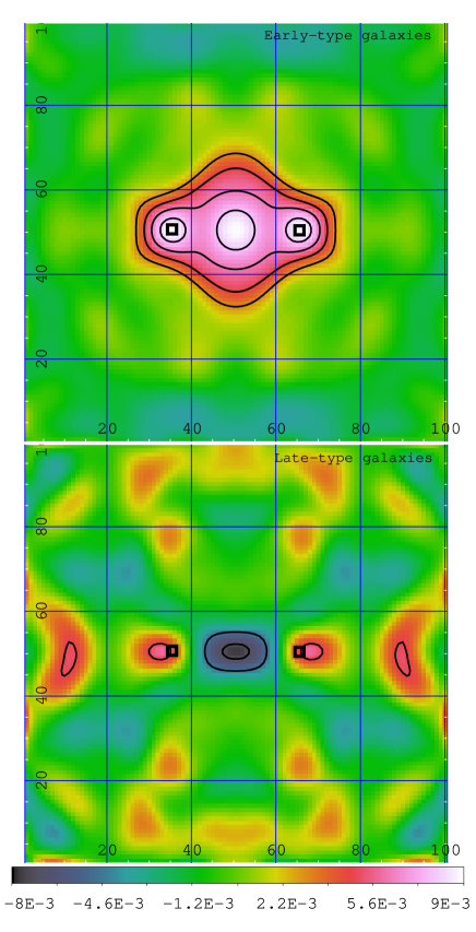
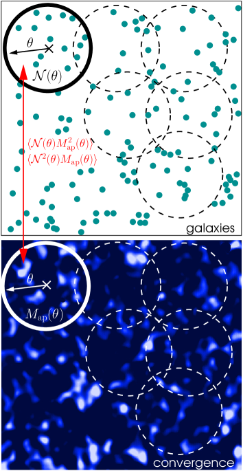
Figure 1: Illustration of the aperture statistics. Fluctuations 𝒩(θ)𝒩𝜃{\cal N}(\theta) in the projected galaxy number density (top panel), smoothed to the characteristic filter scale θ𝜃\theta, are statistically compared to the filtered projected matter fluctuations Map(θ)subscript𝑀ap𝜃M_{\rm ap}(\theta) (lensing convergence; bottom panel). We take 𝒩2(θ)Map(θ)superscript𝒩2𝜃subscript𝑀ap𝜃{\cal N}^{2}(\theta)M_{\rm ap}(\theta) or 𝒩(θ)Map2(θ)𝒩𝜃subscriptsuperscript𝑀2ap𝜃{\cal N}(\theta)M^{2}_{\rm ap}(\theta), and average these for different aperture centres (dashed circles) to estimate third-order moments of the joint probability distribution of 𝒩(θ)𝒩𝜃{\cal N}(\theta) and Map(θ)subscript𝑀ap𝜃M_{\rm ap}(\theta).

For practical purposes, the aperture statistics are a convenient measure for a lensing analysis (Schneider et al., 1998; Schneider, 1998; van Waerbeke, 1998; Crittenden et al., 2002). They quantify moments of fluctuations in κ(𝜽)𝜅𝜽\kappa({\mn@boldsymbol{\theta}}) and κg(𝜽)subscript𝜅g𝜽\kappa_{\rm g}({\mn@boldsymbol{\theta}}) within apertures of a variable angular scale θ𝜃\theta. The moments are determined from the smoothed fields κ(𝜽)𝜅𝜽\kappa({\mn@boldsymbol{\theta}}) and κg(𝜽)subscript𝜅g𝜽\kappa_{\rm g}({\mn@boldsymbol{\theta}}),

Map(θ)subscript𝑀ap𝜃\displaystyle M_{\rm ap}(\theta) =\displaystyle= d2ϑθ2u(|ϑ|θ1)κ(ϑ),superscriptd2italic-ϑsuperscript𝜃2𝑢bold-italic-ϑsuperscript𝜃1𝜅bold-italic-ϑ\displaystyle\int\frac{{\rm d}^{2}\vartheta}{\theta^{2}}\,u\left(|{\mn@boldsymbol{\vartheta}}|\theta^{-1}\right)\,\kappa\left({\mn@boldsymbol{\vartheta}}\right)\;, (6)
𝒩(θ)𝒩𝜃\displaystyle{\cal N}(\theta) =\displaystyle= d2ϑθ2u(|ϑ|θ1)κg(ϑ),superscriptd2italic-ϑsuperscript𝜃2𝑢bold-italic-ϑsuperscript𝜃1subscript𝜅gbold-italic-ϑ\displaystyle\int\frac{{\rm d}^{2}\vartheta}{\theta^{2}}\,u\left(|{\mn@boldsymbol{\vartheta}}|\theta^{-1}\right)\,\kappa_{\rm g}({\mn@boldsymbol{\vartheta}})\;, (7)

where u(ϑ/θ)θ2𝑢italic-ϑ𝜃superscript𝜃2u(\vartheta/\theta)\theta^{-2} is the smoothing kernel. For mathematical convenience, we placed the aperture centre at 𝜽c=0subscript𝜽c0{\mn@boldsymbol{\theta}}_{\rm c}=0 in the previous definition. Third-order moments are defined by considering the ensemble average of

𝒩2Map(θ1;θ2;θ3):=𝒩(θ1)𝒩(θ2)Map(θ3),assigndelimited-⟨⟩superscript𝒩2subscript𝑀apsubscript𝜃1subscript𝜃2subscript𝜃3delimited-⟨⟩𝒩subscript𝜃1𝒩subscript𝜃2subscript𝑀apsubscript𝜃3\displaystyle\langle{\cal N}^{2}M_{\rm ap}\rangle(\theta_{1};\theta_{2};\theta_{3}):=\Big{\langle}{\cal N}(\theta_{1}){\cal N}(\theta_{2})M_{\rm ap}(\theta_{3})\Big{\rangle}\;, (8)
𝒩Map2(θ1;θ2;θ3):=𝒩(θ1)Map(θ2)Map(θ3),assigndelimited-⟨⟩𝒩subscriptsuperscript𝑀2apsubscript𝜃1subscript𝜃2subscript𝜃3delimited-⟨⟩𝒩subscript𝜃1subscript𝑀apsubscript𝜃2subscript𝑀apsubscript𝜃3\displaystyle\langle{\cal N}M^{2}_{\rm ap}\rangle(\theta_{1};\theta_{2};\theta_{3}):=\Big{\langle}{\cal N}(\theta_{1})M_{\rm ap}(\theta_{2})M_{\rm ap}(\theta_{3})\Big{\rangle}\;, (9)

over all random realisations of the fields κ(𝜽)𝜅𝜽\kappa({\mn@boldsymbol{\theta}}) and κg(𝜽)subscript𝜅g𝜽\kappa_{\rm g}({\mn@boldsymbol{\theta}}). Due to the assumed statistical homogeneity of the fields, the averages do not depend on the aperture centre position. Therefore, in practice, where only one realisation or survey is available, these quantities are estimated by averaging the products 𝒩(θ1)𝒩(θ2)Map(θ3)𝒩subscript𝜃1𝒩subscript𝜃2subscript𝑀apsubscript𝜃3{\cal N}(\theta_{1}){\cal N}(\theta_{2})M_{\rm ap}(\theta_{3}) and 𝒩(θ1)Map(θ2)Map(θ3)𝒩subscript𝜃1subscript𝑀apsubscript𝜃2subscript𝑀apsubscript𝜃3{\cal N}(\theta_{1})M_{\rm ap}(\theta_{2})M_{\rm ap}(\theta_{3}) for different aperture centres covering the survey area. See Fig. 1 for an illustration.

For a compensated filter u𝑢u, i.e., 0dθθu(θ)=0superscriptsubscript0differential-d𝜃𝜃𝑢𝜃0\int_{0}^{\infty}{\rm d}\theta\,\theta u(\theta)=0, the aperture mass can in principle be obtained directly from the observable shear through (Schneider et al., 1998)

Map(θ)=002πdφdϑϑθ2q(ϑθ1)(γ(ϑ;φ)),subscript𝑀ap𝜃superscriptsubscript0superscriptsubscript02𝜋d𝜑ditalic-ϑitalic-ϑsuperscript𝜃2𝑞italic-ϑsuperscript𝜃1𝛾bold-italic-ϑ𝜑M_{\rm ap}(\theta)=\int_{0}^{\infty}\int_{0}^{2\pi}\frac{{\rm d}\varphi\,{\rm d}\vartheta\,\vartheta}{\theta^{2}}\,q\left(\vartheta\theta^{-1}\right)\,\Re{\left(\gamma({\mn@boldsymbol{\vartheta}};\varphi)\right)}\;, (10)

where γ(ϑ;φ):=e2iφγc(ϑ)assign𝛾bold-italic-ϑ𝜑superscripte2i𝜑subscript𝛾cbold-italic-ϑ\gamma({\mn@boldsymbol{\vartheta}};\varphi):=-{\rm e}^{-2{\rm i}\varphi}\gamma_{\rm c}({\mn@boldsymbol{\vartheta}}) denotes the Cartesian shear γcsubscript𝛾c\gamma_{\rm c} at angular position ϑbold-italic-ϑ{\mn@boldsymbol{\vartheta}} rotated by the polar angle φ𝜑\varphi. The real part of γ(ϑ;φ)𝛾bold-italic-ϑ𝜑\gamma({\mn@boldsymbol{\vartheta}};\varphi) is the tangential shear, the imaginary part the cross shear. The relation between the filters u(x)𝑢𝑥u(x) and q(x)𝑞𝑥q(x) is given by

q(x)=(2x20xdssu(s))u(x).𝑞𝑥2superscript𝑥2superscriptsubscript0𝑥differential-d𝑠𝑠𝑢𝑠𝑢𝑥q(x)=\left(\frac{2}{x^{2}}\int_{0}^{x}{\rm d}s\,s\,u(s)\right)-u(x)\;. (11)

This paper uses the exponential aperture filter from van Waerbeke (1998), exponential filter hereafter,

u(x)=12π(1x22)ex2/2,𝑢𝑥12𝜋1superscript𝑥22superscriptesuperscript𝑥22u(x)=\frac{1}{2\pi}\left(1-\frac{x^{2}}{2}\right){\rm e}^{-x^{2}/2}\;, (12)

which effectively has a finite support because of the Gaussian factor that suppresses the filter strongly to zero for ϑ3θgreater-than-or-equivalent-toitalic-ϑ3𝜃\vartheta\gtrsim 3\theta (SW05). The Fourier transform of the aperture filter is

u~()=d2θu(θ)e+i𝜽=22e2/2.~𝑢superscriptd2𝜃𝑢𝜃superscripteibold-ℓ𝜽superscript22superscriptesuperscript22\tilde{u}(\ell)=\int{\rm d}^{2}\theta\,u(\theta){\rm e}^{+{\rm i}{\mn@boldsymbol{\ell}}\cdot{\mn@boldsymbol{\theta}}}=\frac{\ell^{2}}{2}{\rm e}^{-\ell^{2}/2}\;. (13)

We generally denote a Fourier transform of f(𝜽)𝑓𝜽f({\mn@boldsymbol{\theta}}) by f~()~𝑓bold-ℓ\tilde{f}({\mn@boldsymbol{\ell}}) in the following. The exponential filter u~()~𝑢\tilde{u}(\ell) peaks in Fourier space at an angular wave number of =22\ell=\sqrt{2}, which determines a characteristic angular scale selected by an aperture radius of θ𝜃\theta.

Refer to caption
Refer to caption
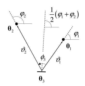
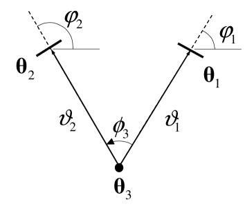
Figure 2: Illustration of the parametrisation of the lens-lens-shear three-point correlator 𝒢~(ϑ1,ϑ2,ϕ3)~𝒢subscriptitalic-ϑ1subscriptitalic-ϑ2subscriptitalic-ϕ3\widetilde{\cal G}(\vartheta_{1},\vartheta_{2},\phi_{3}) (top panel), and the lens-shear-shear correlation function G~±(ϑ1,ϑ2,ϕ3)subscript~𝐺plus-or-minussubscriptitalic-ϑ1subscriptitalic-ϑ2subscriptitalic-ϕ3\widetilde{G}_{\pm}(\vartheta_{1},\vartheta_{2},\phi_{3}) (bottom panel). These statistics are employed to estimate the aperture statistics in Fig. 1. The figure is copied from SW05.

2.3 Aperture statistics estimators

To obtain the third-order moments of the galaxy-matter aperture statistics, we utilise the lens-lens-shear correlation function 𝒢𝒢\cal G in the case of 𝒩2Mapdelimited-⟨⟩superscript𝒩2subscript𝑀ap\langle{\cal N}^{2}M_{\rm ap}\rangle and the lens-shear-shear correlation function G±subscript𝐺plus-or-minusG_{\pm} for 𝒩Map2delimited-⟨⟩𝒩subscriptsuperscript𝑀2ap\langle{\cal N}M^{2}_{\rm ap}\rangle. This section provides only a brief description of this approach. For a more details, its computationally optimised implementation as well as verification, we refer the reader to Sect. 3 of Simon et al. (2008).

In practice, the aperture moments 𝒩2Mapdelimited-⟨⟩superscript𝒩2subscript𝑀ap\langle{\cal N}^{2}M_{\rm ap}\rangle or 𝒩Map2delimited-⟨⟩𝒩subscriptsuperscript𝑀2ap\langle{\cal N}M^{2}_{\rm ap}\rangle are not computed from the aperture mass Mapsubscript𝑀apM_{\rm ap} or aperture number counts 𝒩𝒩\cal N directly. The information contained in the aperture statistics is also contained inside two classes of three-point correlation functions (SW05), which are relatively straightforward to estimate. Once the correlation functions have been determined, they can be transformed to the corresponding aperture statistics by an integral transformation. The estimation process thus proceeds in two basic steps. In the first step, for 𝒩2Mapdelimited-⟨⟩superscript𝒩2subscript𝑀ap\langle{\cal N}^{2}M_{\rm ap}\rangle one estimates the source tangential ellipticity relative to the midpoint connecting two lenses,

𝒢~(ϑ1,ϑ2,ϕ3)=1n¯g2ng(𝜽1)ng(𝜽2)γ(𝜽3;φ1+φ22).~𝒢subscriptitalic-ϑ1subscriptitalic-ϑ2subscriptitalic-ϕ31superscriptsubscript¯𝑛g2delimited-⟨⟩subscript𝑛gsubscript𝜽1subscript𝑛gsubscript𝜽2𝛾subscript𝜽3subscript𝜑1subscript𝜑22\widetilde{{\cal G}}(\vartheta_{1},\vartheta_{2},\phi_{3})=\frac{1}{\overline{n}_{\rm g}^{2}}\Big{\langle}n_{\rm g}({\mn@boldsymbol{\theta}}_{1})n_{\rm g}({\mn@boldsymbol{\theta}}_{2})\gamma\!\left({\mn@boldsymbol{\theta}}_{3};\frac{\varphi_{1}+\varphi_{2}}{2}\right)\Big{\rangle}\;. (14)

The meaning of the notation is illustrated in the left panel of Fig. 2. For 𝒩Map2delimited-⟨⟩𝒩subscriptsuperscript𝑀2ap\langle{\cal N}M^{2}_{\rm ap}\rangle one estimates the correlation of the ellipticities of two sources relative to the line connecting the sources as a function of separation from one lens (right panel),

G~±(ϑ1,ϑ2,ϕ3)=1n¯gγ(𝜽1;φ1)γ±(𝜽2;φ2)ng(𝜽3).subscript~𝐺plus-or-minussubscriptitalic-ϑ1subscriptitalic-ϑ2subscriptitalic-ϕ31subscript¯𝑛gdelimited-⟨⟩𝛾subscript𝜽1subscript𝜑1superscript𝛾plus-or-minussubscript𝜽2subscript𝜑2subscript𝑛gsubscript𝜽3\widetilde{G}_{\pm}(\vartheta_{1},\vartheta_{2},\phi_{3})=\frac{1}{\overline{n}_{\rm g}}\Big{\langle}\gamma({\mn@boldsymbol{\theta}}_{1};\varphi_{1})\gamma^{\pm}({\mn@boldsymbol{\theta}}_{2};\varphi_{2})n_{\rm g}({\mn@boldsymbol{\theta}}_{3})\Big{\rangle}\;. (15)

Here and in the following equations a superscript “±plus-or-minus\pm” as in γ±superscript𝛾plus-or-minus\gamma^{\pm} means γ𝛾\gamma for γsuperscript𝛾\gamma^{-} (in case of G~subscript~𝐺\widetilde{G}_{-}) and the complex conjugate γsuperscript𝛾\gamma^{\ast} for γ+superscript𝛾\gamma^{+} (in case of G~+subscript~𝐺\widetilde{G}_{+}).

Both correlation functions are estimated inside bins of similar triangles, i.e., lens-source triples within a configuration of comparable side lengths ϑ1,2subscriptitalic-ϑ12\vartheta_{1,2} and opening angles ϕ3subscriptitalic-ϕ3\phi_{3}, by summing over all relevant galaxy triplets. Any triple of three galaxy positions 𝜽i,𝜽j,𝜽ksubscript𝜽𝑖subscript𝜽𝑗subscript𝜽𝑘{\mn@boldsymbol{\theta}}_{i},{\mn@boldsymbol{\theta}}_{j},{\mn@boldsymbol{\theta}}_{k} that meets the criteria of a relevant triangle is flagged by Δijkϑ1ϑ2ϕ3=1superscriptsubscriptΔ𝑖𝑗𝑘subscriptitalic-ϑ1subscriptitalic-ϑ2subscriptitalic-ϕ31\Delta_{ijk}^{\vartheta_{1}\vartheta_{2}\phi_{3}}=1 and Δijkϑ1ϑ2ϕ3=0superscriptsubscriptΔ𝑖𝑗𝑘subscriptitalic-ϑ1subscriptitalic-ϑ2subscriptitalic-ϕ30\Delta_{ijk}^{\vartheta_{1}\vartheta_{2}\phi_{3}}=0 otherwise. For this study, we utilise 100 logarithmic bins for both ϑ1subscriptitalic-ϑ1\vartheta_{1} and ϑ2subscriptitalic-ϑ2\vartheta_{2}, and 100 linear bins for the opening angle ϕ3subscriptitalic-ϕ3\phi_{3}. For estimating 𝒢~~𝒢\widetilde{\cal G} we utilise

𝒢~est(ϑ1,ϑ2,ϕ3)=superscript~𝒢estsubscriptitalic-ϑ1subscriptitalic-ϑ2subscriptitalic-ϕ3absent\displaystyle\widetilde{\cal G}^{\rm est}(\vartheta_{1},\vartheta_{2},\phi_{3})=
i=1Ndj=1Ndk=1Nswkϵkei(φi+φj)[1+ω(|𝜽i𝜽j|)]Δijkϑ1ϑ2ϕ3i=1Ndj=1Ndk=1NswkΔijkϑ1ϑ2ϕ3,superscriptsubscript𝑖1subscript𝑁dsuperscriptsubscript𝑗1subscript𝑁dsuperscriptsubscript𝑘1subscript𝑁ssubscript𝑤𝑘subscriptitalic-ϵ𝑘superscripteisubscript𝜑𝑖subscript𝜑𝑗delimited-[]1𝜔subscript𝜽𝑖subscript𝜽𝑗superscriptsubscriptΔ𝑖𝑗𝑘subscriptitalic-ϑ1subscriptitalic-ϑ2subscriptitalic-ϕ3superscriptsubscript𝑖1subscript𝑁dsuperscriptsubscript𝑗1subscript𝑁dsuperscriptsubscript𝑘1subscript𝑁ssubscript𝑤𝑘superscriptsubscriptΔ𝑖𝑗𝑘subscriptitalic-ϑ1subscriptitalic-ϑ2subscriptitalic-ϕ3\displaystyle\!\!\!\!\frac{-\sum\limits_{i=1}^{N_{\rm d}}\sum\limits_{j=1}^{N_{\rm d}}\sum\limits_{k=1}^{N_{\rm s}}w_{k}\,\epsilon_{k}\,{\rm e}^{-{\rm i}(\varphi_{i}+\varphi_{j})}\big{[}1+\omega(|{\mn@boldsymbol{\theta}}_{i}-{\mn@boldsymbol{\theta}}_{j}|)\big{]}\Delta_{ijk}^{\vartheta_{1}\vartheta_{2}\phi_{3}}}{\sum\limits_{i=1}^{N_{\rm d}}\sum\limits_{j=1}^{N_{\rm d}}\sum\limits_{k=1}^{N_{\rm s}}w_{k}\Delta_{ijk}^{\vartheta_{1}\vartheta_{2}\phi_{3}}}\;,

and for G~±subscript~𝐺plus-or-minus\widetilde{G}_{\pm} the estimator

G~±est(ϑ1,ϑ2,ϕ3)=subscriptsuperscript~𝐺estplus-or-minussubscriptitalic-ϑ1subscriptitalic-ϑ2subscriptitalic-ϕ3absent\displaystyle\widetilde{G}^{\rm est}_{\pm}(\vartheta_{1},\vartheta_{2},\phi_{3})=
i=1Ndj=1Nsk=1Nswjwkϵjϵk±e2iφje±2iφkΔijkϑ1ϑ2ϕ3i=1Ndj=1Nsk=1NswjwkΔijkϑ1ϑ2ϕ3,superscriptsubscript𝑖1subscript𝑁dsuperscriptsubscript𝑗1subscript𝑁ssuperscriptsubscript𝑘1subscript𝑁ssubscript𝑤𝑗subscript𝑤𝑘subscriptitalic-ϵ𝑗superscriptsubscriptitalic-ϵ𝑘plus-or-minussuperscripte2isubscript𝜑𝑗superscripteplus-or-minus2isubscript𝜑𝑘superscriptsubscriptΔ𝑖𝑗𝑘subscriptitalic-ϑ1subscriptitalic-ϑ2subscriptitalic-ϕ3superscriptsubscript𝑖1subscript𝑁dsuperscriptsubscript𝑗1subscript𝑁ssuperscriptsubscript𝑘1subscript𝑁ssubscript𝑤𝑗subscript𝑤𝑘superscriptsubscriptΔ𝑖𝑗𝑘subscriptitalic-ϑ1subscriptitalic-ϑ2subscriptitalic-ϕ3\displaystyle\frac{\sum\limits_{i=1}^{N_{\rm d}}\sum\limits_{j=1}^{N_{\rm s}}\sum\limits_{k=1}^{N_{\rm s}}w_{j}\,w_{k}\,\epsilon_{j}\epsilon_{k}^{\pm}{\rm e}^{-2{\rm i}\varphi_{j}}{\rm e}^{\pm 2{\rm i}\varphi_{k}}\Delta_{ijk}^{\vartheta_{1}\vartheta_{2}\phi_{3}}}{\sum\limits_{i=1}^{N_{\rm d}}\sum\limits_{j=1}^{N_{\rm s}}\sum\limits_{k=1}^{N_{\rm s}}w_{j}\,w_{k}\Delta_{ijk}^{\vartheta_{1}\vartheta_{2}\phi_{3}}}\;,

where Ndsubscript𝑁dN_{\rm d} and Nssubscript𝑁sN_{\rm s} are the number of lenses and sources, wisubscript𝑤𝑖w_{i} are statistical weights of sources, φisubscript𝜑𝑖\varphi_{i} are polar angles of the position vectors of galaxies with respect to the coordinate origin, ϵisubscriptitalic-ϵ𝑖\epsilon_{i} are the source ellipticities, and

ω(|𝚫𝜽|)=κg(𝜽)κg(𝜽+𝚫𝜽)𝜔𝚫𝜽delimited-⟨⟩subscript𝜅g𝜽subscript𝜅g𝜽𝚫𝜽\omega(|{\mn@boldsymbol{\Delta\theta}}|)=\Big{\langle}\kappa_{\rm g}({\mn@boldsymbol{\theta}})\kappa_{\rm g}({\mn@boldsymbol{\theta}}+{\mn@boldsymbol{\Delta\theta}})\Big{\rangle} (18)

is the angular two-point clustering of the lenses (e.g. Peebles, 1980). In this paper, the angular clustering of lenses is estimated by means of the estimator in Landy & Szalay (1993) prior to the estimation of 𝒢~~𝒢\widetilde{\cal G} and then interpolated. Sources are weighed by the inverse-variance uncertainty in the lensfit ellipticity measurement (Miller et al., 2012).

In a second step, we transform the estimates of 𝒢~~𝒢\widetilde{\cal G} and G~±subscript~𝐺plus-or-minus\widetilde{G}_{\pm} to the aperture statistics by devising the transformation integrals Eqs. (63), (57), and (59) in SW05. There is no need to remove the unconnected terms in the correlation functions. As shown in SW05 (Sect. 7.2. therein), the transformation from 𝒢𝒢{\cal G} to 𝒩2Mapdelimited-⟨⟩superscript𝒩2subscript𝑀ap\langle{\cal N}^{2}M_{\rm ap}\rangle yields the same result when 𝒢~~𝒢\widetilde{\cal G} is taken instead of 𝒢𝒢\cal G. Therefore, the integral transformation automatically ignores unconnected second-order terms in the triple correlator, resulting in an aperture statistics that are only determined by pure (connected) third-order correlation terms. The same holds true for G~±subscript~𝐺plus-or-minus\widetilde{G}_{\pm} and 𝒩Map2delimited-⟨⟩𝒩subscriptsuperscript𝑀2ap\langle{\cal N}M^{2}_{\rm ap}\rangle.

2.4 Relation to 3D galaxy-matter bispectra

The aperture statistics are directly connected to the angular cross-bispectra of the projected matter and lens distribution:

𝒩2Map(θ1;θ2;θ3)=delimited-⟨⟩superscript𝒩2subscript𝑀apsubscript𝜃1subscript𝜃2subscript𝜃3absent\displaystyle\langle{\cal N}^{2}M_{\rm ap}\rangle(\theta_{1};\theta_{2};\theta_{3})=
d21(2π)2d22(2π)2u~(1θ1)u~(2θ2)u~(|𝟏+2|θ3)bggκ(𝟏,𝟐),superscriptd2subscript1superscript2𝜋2superscriptd2subscript2superscript2𝜋2~𝑢subscript1subscript𝜃1~𝑢subscript2subscript𝜃2~𝑢subscriptbold-ℓ1subscriptbold-ℓ2subscript𝜃3subscript𝑏gg𝜅subscriptbold-ℓ1subscriptbold-ℓ2\displaystyle\!\!\!\!\!\!\!\!\int\frac{{\rm d}^{2}\ell_{1}}{(2\pi)^{2}}\int\frac{{\rm d}^{2}\ell_{2}}{(2\pi)^{2}}\tilde{u}(\ell_{1}\theta_{1})\tilde{u}(\ell_{2}\theta_{2})\tilde{u}(|{\mn@boldsymbol{\ell_{1}}}+{\mn@boldsymbol{\ell}}_{2}|\theta_{3})b_{{\rm gg}\kappa}({\mn@boldsymbol{\ell_{1}}},{\mn@boldsymbol{\ell_{2}}})\;,
𝒩Map2(θ1;θ2;θ3)=delimited-⟨⟩𝒩subscriptsuperscript𝑀2apsubscript𝜃1subscript𝜃2subscript𝜃3absent\displaystyle\langle{\cal N}M^{2}_{\rm ap}\rangle(\theta_{1};\theta_{2};\theta_{3})=
d21(2π)2d22(2π)2u~(1θ1)u~(2θ2)u~(|𝟏+2|θ3)bκκg(𝟏,𝟐),superscriptd2subscript1superscript2𝜋2superscriptd2subscript2superscript2𝜋2~𝑢subscript1subscript𝜃1~𝑢subscript2subscript𝜃2~𝑢subscriptbold-ℓ1subscriptbold-ℓ2subscript𝜃3subscript𝑏𝜅𝜅gsubscriptbold-ℓ1subscriptbold-ℓ2\displaystyle\!\!\!\!\!\!\!\!\int\frac{{\rm d}^{2}\ell_{1}}{(2\pi)^{2}}\int\frac{{\rm d}^{2}\ell_{2}}{(2\pi)^{2}}\tilde{u}(\ell_{1}\theta_{1})\tilde{u}(\ell_{2}\theta_{2})\tilde{u}(|{\mn@boldsymbol{\ell_{1}}}+{\mn@boldsymbol{\ell}}_{2}|\theta_{3})b_{\kappa\kappa{\rm g}}({\mn@boldsymbol{\ell_{1}}},{\mn@boldsymbol{\ell_{2}}})\;,

where the angular galaxy-galaxy-matter bispectrum is

κ~g(1)κ~g(2)κ~(3)=(2π)2δD(2)(1+2+3)bggκ(𝟏,𝟐)delimited-⟨⟩subscript~𝜅gsubscriptbold-ℓ1subscript~𝜅gsubscriptbold-ℓ2~𝜅subscriptbold-ℓ3superscript2𝜋2subscriptsuperscript𝛿2Dsubscriptbold-ℓ1subscriptbold-ℓ2subscriptbold-ℓ3subscript𝑏gg𝜅subscriptbold-ℓ1subscriptbold-ℓ2\langle\tilde{\kappa}_{\rm g}({\mn@boldsymbol{\ell}}_{1})\tilde{\kappa}_{\rm g}({\mn@boldsymbol{\ell}}_{2})\tilde{\kappa}({\mn@boldsymbol{\ell}}_{3})\rangle=(2\pi)^{2}\delta^{(2)}_{\rm D}({\mn@boldsymbol{\ell}}_{1}+{\mn@boldsymbol{\ell}}_{2}+{\mn@boldsymbol{\ell}}_{3})b_{{\rm gg}\kappa}({\mn@boldsymbol{\ell_{1}}},{\mn@boldsymbol{\ell_{2}}}) (21)

and the angular matter-matter-galaxy bispectrum is

κ~(1)κ~(2)κ~g(3)=(2π)2δD(2)(1+2+3)bκκg(𝟏,𝟐).delimited-⟨⟩~𝜅subscriptbold-ℓ1~𝜅subscriptbold-ℓ2subscript~𝜅gsubscriptbold-ℓ3superscript2𝜋2subscriptsuperscript𝛿2Dsubscriptbold-ℓ1subscriptbold-ℓ2subscriptbold-ℓ3subscript𝑏𝜅𝜅gsubscriptbold-ℓ1subscriptbold-ℓ2\langle\tilde{\kappa}({\mn@boldsymbol{\ell}}_{1})\tilde{\kappa}({\mn@boldsymbol{\ell}}_{2})\tilde{\kappa}_{\rm g}({\mn@boldsymbol{\ell}}_{3})\rangle=(2\pi)^{2}\delta^{(2)}_{\rm D}({\mn@boldsymbol{\ell}}_{1}+{\mn@boldsymbol{\ell}}_{2}+{\mn@boldsymbol{\ell}}_{3})b_{\kappa\kappa{\rm g}}({\mn@boldsymbol{\ell_{1}}},{\mn@boldsymbol{\ell_{2}}})\;. (22)

For statistically homogeneous random fields, the triple correlators on the left-hand side of the previous two equations can only be non-vanishing when 1+2+3=𝟎subscriptbold-ℓ1subscriptbold-ℓ2subscriptbold-ℓ30{\mn@boldsymbol{\ell}}_{1}+{\mn@boldsymbol{\ell}}_{2}+{\mn@boldsymbol{\ell}}_{3}={\mn@boldsymbol{0}}, which is reflected by the 2D Dirac delta functions δD(2)(𝒙)subscriptsuperscript𝛿2D𝒙\delta^{(2)}_{\rm D}({\mn@boldsymbol{x}}) on the right-hand sides. Owing to homogeneity, the bispectra thus depend only on two independent arguments bold-ℓ{\mn@boldsymbol{\ell}}, for which we arbitrarily choose 1subscriptbold-ℓ1{\mn@boldsymbol{\ell}}_{1} and 2subscriptbold-ℓ2{\mn@boldsymbol{\ell}}_{2}. This automatically implies 3=(1+2)subscriptbold-ℓ3subscriptbold-ℓ1subscriptbold-ℓ2{\mn@boldsymbol{\ell}}_{3}=-({\mn@boldsymbol{\ell}}_{1}+{\mn@boldsymbol{\ell}}_{2}). In addition the statistical isotropy implies that the bispectra are solely functions of the moduli of 1,2subscriptbold-ℓ12{\mn@boldsymbol{\ell}}_{1,2} and the angle enclosed by both wave vectors.

As can be seen from Eqs. (2.4), (2.4), the aperture statistics are a locally filtered version of the bispectrum because the exponential u𝑢u-filter is relatively localised in \ell-space with a filter maximum at max=2/θsubscriptmax2𝜃\ell_{\rm max}=\sqrt{2}/\theta. By means of the filtering, the aperture statistics basically becomes a band power bispectrum version of bggκsubscript𝑏gg𝜅b_{{\rm gg}\kappa} or bκκgsubscript𝑏𝜅𝜅gb_{\kappa\kappa\rm g}. Hence the aperture statistics Eqs. (8), (9) measure two different angular galaxy-matter band power cross-bispectra.

By virtue of the Limber approximation (Kaiser, 1992; Bartelmann & Schneider, 2001) the angular bispectra and thereby the aperture statistics Eqs. (2.4), (2.4) can directly be related to the 3D cross-bispectrum of the matter and lens distribution (SW05) as primary physical quantities that are assessed by the statistics:

bggκ(1,2)=subscript𝑏gg𝜅subscriptbold-ℓ1subscriptbold-ℓ2absent\displaystyle b_{{\rm gg}\kappa}({\mn@boldsymbol{\ell}}_{1},{\mn@boldsymbol{\ell}}_{2})=
3Ωm2DH20χhdχg(χ)pf2(χ)fK3(χ)a(χ)Bggm(1fK(χ),2fK(χ),χ),3subscriptΩm2superscriptsubscript𝐷H2superscriptsubscript0subscript𝜒hdifferential-d𝜒𝑔𝜒superscriptsubscript𝑝f2𝜒subscriptsuperscript𝑓3K𝜒𝑎𝜒subscript𝐵ggmsubscriptbold-ℓ1subscript𝑓K𝜒subscriptbold-ℓ2subscript𝑓K𝜒𝜒\displaystyle\frac{3\Omega_{\rm m}}{2D_{\rm H}^{2}}\int_{0}^{\chi_{\rm h}}{\rm d}\chi\,\frac{g(\chi)p_{\rm f}^{2}(\chi)}{f^{3}_{\rm K}(\chi)a(\chi)}B_{\rm ggm}\big{(}\frac{{\mn@boldsymbol{\ell}}_{1}}{f_{\rm K}(\chi)},\frac{{\mn@boldsymbol{\ell}}_{2}}{f_{\rm K}(\chi)},\chi\big{)}\;,
bκκg(1,2)=subscript𝑏𝜅𝜅gsubscriptbold-ℓ1subscriptbold-ℓ2absent\displaystyle b_{\kappa\kappa\rm g}({\mn@boldsymbol{\ell}}_{1},{\mn@boldsymbol{\ell}}_{2})=
9Ωm24DH40χhdχg2(χ)pf(χ)fK2(χ)a2(χ)Bmmg(1fK(χ),2fK(χ),χ),9subscriptsuperscriptΩ2m4superscriptsubscript𝐷H4superscriptsubscript0subscript𝜒hdifferential-d𝜒superscript𝑔2𝜒subscript𝑝f𝜒subscriptsuperscript𝑓2K𝜒superscript𝑎2𝜒subscript𝐵mmgsubscriptbold-ℓ1subscript𝑓K𝜒subscriptbold-ℓ2subscript𝑓K𝜒𝜒\displaystyle\frac{9\Omega^{2}_{\rm m}}{4D_{\rm H}^{4}}\int_{0}^{\chi_{\rm h}}{\rm d}\chi\,\frac{g^{2}(\chi)p_{\rm f}(\chi)}{f^{2}_{\rm K}(\chi)a^{2}(\chi)}B_{\rm mmg}\big{(}\frac{{\mn@boldsymbol{\ell}}_{1}}{f_{\rm K}(\chi)},\frac{{\mn@boldsymbol{\ell}}_{2}}{f_{\rm K}(\chi)},\chi\big{)}\;,

where the 3D bispectra are determined by the Fourier transforms of the matter density contrast, δ~m(𝒌,χ)subscript~𝛿m𝒌𝜒\tilde{\delta}_{\rm m}({\mn@boldsymbol{k}},\chi), and galaxy number density contrast, δ~g(𝒌,χ)subscript~𝛿g𝒌𝜒\tilde{\delta}_{\rm g}({\mn@boldsymbol{k}},\chi), at radial distance χ𝜒\chi, namely

δ~g(𝒌1,χ)δ~g(𝒌2,χ)δ~m(𝒌3,χ)=delimited-⟨⟩subscript~𝛿gsubscript𝒌1𝜒subscript~𝛿gsubscript𝒌2𝜒subscript~𝛿msubscript𝒌3𝜒absent\displaystyle\langle\tilde{\delta}_{\rm g}({\mn@boldsymbol{k}}_{1},\chi)\tilde{\delta}_{\rm g}({\mn@boldsymbol{k}}_{2},\chi)\tilde{\delta}_{\rm m}({\mn@boldsymbol{k}}_{3},\chi)\rangle=
(2π)3δD(3)(𝒌1+𝒌2+𝒌3)Bggm(𝒌1,𝒌2,χ),superscript2𝜋3subscriptsuperscript𝛿3Dsubscript𝒌1subscript𝒌2subscript𝒌3subscript𝐵ggmsubscript𝒌1subscript𝒌2𝜒\displaystyle(2\pi)^{3}\delta^{(3)}_{\rm D}({\mn@boldsymbol{k}}_{1}+{\mn@boldsymbol{k}}_{2}+{\mn@boldsymbol{k}}_{3})B_{\rm ggm}({\mn@boldsymbol{k}}_{1},{\mn@boldsymbol{k}}_{2},\chi)\;,
δ~m(𝒌1,χ)δ~m(𝒌2,χ)δ~g(𝒌3,χ)=delimited-⟨⟩subscript~𝛿msubscript𝒌1𝜒subscript~𝛿msubscript𝒌2𝜒subscript~𝛿gsubscript𝒌3𝜒absent\displaystyle\langle\tilde{\delta}_{\rm m}({\mn@boldsymbol{k}}_{1},\chi)\tilde{\delta}_{\rm m}({\mn@boldsymbol{k}}_{2},\chi)\tilde{\delta}_{\rm g}({\mn@boldsymbol{k}}_{3},\chi)\rangle=
(2π)3δD(3)(𝒌1+𝒌2+𝒌3)Bmmg(𝒌1,𝒌2,χ).superscript2𝜋3subscriptsuperscript𝛿3Dsubscript𝒌1subscript𝒌2subscript𝒌3subscript𝐵mmgsubscript𝒌1subscript𝒌2𝜒\displaystyle(2\pi)^{3}\delta^{(3)}_{\rm D}({\mn@boldsymbol{k}}_{1}+{\mn@boldsymbol{k}}_{2}+{\mn@boldsymbol{k}}_{3})B_{\rm mmg}({\mn@boldsymbol{k}}_{1},{\mn@boldsymbol{k}}_{2},\chi)\;.

The vector 𝒌𝒌{\mn@boldsymbol{k}} is the comoving wave number of modes entering the triple correlator. As before with the angular bispectra, the spatial bispectra are also isotropic, i.e., they are only functions of |𝒌1|subscript𝒌1|{\mn@boldsymbol{k}}_{1}|, |𝒌2|subscript𝒌2|{\mn@boldsymbol{k}}_{2}| and the angle spanned by 𝒌1subscript𝒌1{\mn@boldsymbol{k}}_{1} and 𝒌2subscript𝒌2{\mn@boldsymbol{k}}_{2}.

To refine the previous RCS1 measurement in Simon et al. (2008) for different galaxy populations, we focus on equally-sized apertures with θ1=θ2=θ3subscript𝜃1subscript𝜃2subscript𝜃3\theta_{1}=\theta_{2}=\theta_{3} only. This leads us to the short hand notations 𝒩2Map(θ):=𝒩2Map(θ;θ;θ)assigndelimited-⟨⟩superscript𝒩2subscript𝑀ap𝜃delimited-⟨⟩superscript𝒩2subscript𝑀ap𝜃𝜃𝜃\langle{\cal N}^{2}M_{\rm ap}\rangle(\theta):=\langle{\cal N}^{2}M_{\rm ap}\rangle(\theta;\theta;\theta), likewise for 𝒩Map2delimited-⟨⟩𝒩superscriptsubscript𝑀ap2\langle{\cal N}M_{\rm ap}^{2}\rangle. Due to the action of the u𝑢u-filter in the Eqs. (2.4) and (2.4) this picks up mainly bispectrum contributions from equilateral triangles |1|=|2|=|1+2|subscriptbold-ℓ1subscriptbold-ℓ2subscriptbold-ℓ1subscriptbold-ℓ2|{\mn@boldsymbol{\ell}}_{1}|=|{\mn@boldsymbol{\ell}}_{2}|=|{\mn@boldsymbol{\ell}}_{1}+{\mn@boldsymbol{\ell}}_{2}|, albeit also mixing in signal from other triangles because of the finite width of the u𝑢u-filter in \ell-space.

2.5 Systematics indicators

The gravitational shear of distant galaxy images is produced by small fluctuations δϕ𝛿italic-ϕ\delta\phi in the intervening gravitational potential. To lowest order in δϕ/c2𝛿italic-ϕsuperscript𝑐2\delta\phi/c^{2} this is expected to only produce curl-free shear fields (B-modes vanish). Current surveys do not have the power to measure higher-order effects, such that we expect these to be undetectable in our data. Shear-related correlation functions, or aperture moments involving the aperture mass, hence vanish after rotation of all sources by 45superscript4545^{\circ}, i.e., after γc(𝜽)iγc(𝜽)maps-tosubscript𝛾c𝜽isubscript𝛾c𝜽\gamma_{\rm c}({\mn@boldsymbol{\theta}})\mapsto-{\rm i}\,\gamma_{\rm c}{\mn@boldsymbol{(}}{\mn@boldsymbol{\theta}}). Translated into data analysis, a 45superscript4545^{\circ} rotation of the source ellipticities should result in a measurement that is statistically consistent with the experimental noise (e.g. Hetterscheidt et al., 2007). We use this as a necessary (but not sufficient) indicator for the absence of systematics in the data.

The estimator G~±estsubscriptsuperscript~𝐺estplus-or-minus\widetilde{G}^{\rm est}_{\pm} in Eq. (2.3) incorporates two sources with two uniquely different possibilities to probe systematics: rotating the ellipticities ϵjsubscriptitalic-ϵ𝑗\epsilon_{j} and ϵksubscriptitalic-ϵ𝑘\epsilon_{k} of both sources results in the so-called B-mode channel of 𝒩Map2(θ)delimited-⟨⟩𝒩subscriptsuperscript𝑀2ap𝜃\langle{\cal N}M^{2}_{\rm ap}\rangle(\theta), denoted here by 𝒩M2(θ)delimited-⟨⟩𝒩superscriptsubscript𝑀perpendicular-to2𝜃\langle{\cal N}M_{\perp}^{2}\rangle(\theta), and the P-mode channel, 𝒩MMap(θ)delimited-⟨⟩𝒩subscript𝑀perpendicular-tosubscript𝑀ap𝜃\langle{\cal N}M_{\perp}M_{\rm ap}\rangle(\theta), if only either ϵjsubscriptitalic-ϵ𝑗\epsilon_{j} or ϵksubscriptitalic-ϵ𝑘\epsilon_{k} are rotated. As pointed out by Schneider (2003), a P-mode is a signature of a parity-invariance violation in the shear data, which in a parity-invariant universe can only be generated by systematics in the PSF correction pipeline, or in the algorithm for the statistical analysis of the data. Non-vanishing B-modes, on the other hand, can have a physical cause. For example, they can be associated with the intrinsic clustering of sources (Schneider et al., 2002), intrinsic alignment correlations of physically close sources or intrinsic shape-shear correlations (Heymans et al., 2006, and references therein). Especially the latter two are a concern for this analysis, as these effects are known to affect the E-mode channel of the aperture statistics, which is the prime focus of this work. However, currently it is unclear by how much this really affects G3L. We discuss in the following Sect. 2.6 that the influence of these systematics can be suppressed by separating lenses and sources in redshift, which is carried out in our analysis.

Since the estimator 𝒢~estsuperscript~𝒢est\widetilde{\cal G}^{\rm est} in Eq. (2.3) involves one source, there is only a single systematics indicator of 𝒩2Map(θ)delimited-⟨⟩superscript𝒩2subscript𝑀ap𝜃\langle{\cal N}^{2}M_{\rm ap}\rangle(\theta), which is a parity violation indicator, a P-mode channel. In the following we will denote these statistics as 𝒩2M(θ)delimited-⟨⟩superscript𝒩2subscript𝑀perpendicular-to𝜃\langle{\cal N}^{2}M_{\perp}\rangle(\theta). As shown in SW05, the B- and P-modes of the statistics can be computed from 𝒢~~𝒢\widetilde{\cal G} and G~±subscript~𝐺plus-or-minus\widetilde{G}_{\pm} directly by utilising an alternative integral kernel in the transformation from correlation functions to aperture statistics; see their Sect. 7.1 and 7.2.

2.6 Reduction of II- and GI-contributions

One possible source of systematics are correlations with intrinsic ellipticities ϵssubscriptitalic-ϵs\epsilon_{\rm s} of sources. A correlation between ϵssubscriptitalic-ϵs\epsilon_{\rm s} of different sources (II-correlations) or between ϵssubscriptitalic-ϵs\epsilon_{\rm s} and a fluctuation in the mass density field generating shear (GI-correlations) is known to contribute to the shear correlation functions (e.g Hirata & Seljak, 2004; Heymans et al., 2006; Joachimi et al., 2011). For a discussion of intrinsic alignments in CFHTLenS see also Heymans et al. (2012). We argue here that selecting lenses and sources from well separated distances ideally removes contaminations by II- or GI-correlations in the G3L statistics.

Consider the galaxy number density contrasts κg,1subscript𝜅g1\kappa_{{\rm g},1} and κg,2subscript𝜅g2\kappa_{{\rm g},2} in two arbitrary line-of-sight directions 𝜽1subscript𝜽1{\mn@boldsymbol{\theta}}_{1} and 𝜽2subscript𝜽2{\mn@boldsymbol{\theta}}_{2}, respectively, and a source ellipticity ϵs+γsubscriptitalic-ϵs𝛾\epsilon_{\rm s}+\gamma in a third direction 𝜽3subscript𝜽3{\mn@boldsymbol{\theta}}_{3}. The shear γ𝛾\gamma and ϵssubscriptitalic-ϵs\epsilon_{\rm s} are rotated in direction of the mid-point between the two lenses according to the definition of 𝒢𝒢\cal G. If lenses and sources are well separated in distance, then their properties are statistically independent. The lens-lens-shear correlator measures

𝒢𝒢\displaystyle{\cal G} =\displaystyle= κg,1κg,2(γ+ϵs)delimited-⟨⟩subscript𝜅g1subscript𝜅g2𝛾subscriptitalic-ϵs\displaystyle\langle\kappa_{{\rm g},1}\kappa_{{\rm g},2}(\gamma+\epsilon_{\rm s})\rangle
=\displaystyle= κg,1κg,2γ+κg,1κg,2ϵsdelimited-⟨⟩subscript𝜅g1subscript𝜅g2𝛾delimited-⟨⟩subscript𝜅g1subscript𝜅g2delimited-⟨⟩subscriptitalic-ϵs\displaystyle\langle\kappa_{{\rm g},1}\kappa_{{\rm g},2}\gamma\rangle+\langle\kappa_{{\rm g},1}\kappa_{{\rm g},2}\rangle\langle\epsilon_{\rm s}\rangle
=\displaystyle= κg,1κg,2γ,delimited-⟨⟩subscript𝜅g1subscript𝜅g2𝛾\displaystyle\langle\kappa_{{\rm g},1}\kappa_{{\rm g},2}\gamma\rangle\;,

free of any systematic contribution from the intrinsic shape ϵssubscriptitalic-ϵs\epsilon_{\rm s}, if ϵssubscriptitalic-ϵs\epsilon_{\rm s} is statistically independent of the lens number density fluctuation κgsubscript𝜅g\kappa_{\rm g}, i.e.,

κg,1κg,2ϵs=κg,1κg,2ϵs,delimited-⟨⟩subscript𝜅g1subscript𝜅g2subscriptitalic-ϵsdelimited-⟨⟩subscript𝜅g1subscript𝜅g2delimited-⟨⟩subscriptitalic-ϵs\langle\kappa_{{\rm g},1}\kappa_{{\rm g},2}\epsilon_{\rm s}\rangle=\langle\kappa_{{\rm g},1}\kappa_{{\rm g},2}\rangle\langle\epsilon_{\rm s}\rangle\;, (28)

vanishing due to ϵs=0delimited-⟨⟩subscriptitalic-ϵs0\langle\epsilon_{\rm s}\rangle=0.

Now, consider a lens number density contrast κgsubscript𝜅g\kappa_{\rm g} in one direction and the ellipticities ϵs,i+γisubscriptitalic-ϵs𝑖subscript𝛾𝑖\epsilon_{{\rm s},i}+\gamma_{i} of two source images i=1,2𝑖12i=1,2 in two other directions. The ellipticities are rotated in direction of line connecting the sources in accordance with the definition of G±subscript𝐺plus-or-minusG_{\pm}. The triple correlator measures

G±subscript𝐺plus-or-minus\displaystyle G_{\pm} =\displaystyle= κg(γ1±+ϵs,1±)(γ2+ϵs,2)delimited-⟨⟩subscript𝜅gsubscriptsuperscript𝛾plus-or-minus1subscriptsuperscriptitalic-ϵplus-or-minuss1subscript𝛾2subscriptitalic-ϵs2\displaystyle\langle\kappa_{\rm g}(\gamma^{\pm}_{1}+\epsilon^{\pm}_{{\rm s},1})(\gamma_{2}+\epsilon_{{\rm s},2})\rangle
=\displaystyle= κgγ1±γ2+κgϵs,1±γ2+κgγ1±ϵs,2+κgϵs,1±ϵs,2delimited-⟨⟩subscript𝜅gsubscriptsuperscript𝛾plus-or-minus1subscript𝛾2delimited-⟨⟩subscript𝜅gsubscriptsuperscriptitalic-ϵplus-or-minussubscripts,1subscript𝛾2delimited-⟨⟩subscript𝜅gsubscriptsuperscript𝛾plus-or-minus1subscriptitalic-ϵs2delimited-⟨⟩subscript𝜅gsuperscriptsubscriptitalic-ϵs1plus-or-minussubscriptitalic-ϵs2\displaystyle\langle\kappa_{\rm g}\gamma^{\pm}_{1}\gamma_{2}\rangle+\langle\kappa_{\rm g}\epsilon^{\pm}_{{\rm s}_{,}1}\gamma_{2}\rangle+\langle\kappa_{\rm g}\gamma^{\pm}_{1}\epsilon_{{\rm s},2}\rangle+\langle\kappa_{\rm g}\epsilon_{{\rm s},1}^{\pm}\epsilon_{{\rm s},2}\rangle
=\displaystyle= κgγ1±γ2+κgϵs,1±γ2+κgγ1±ϵs,2+κgϵs,1±ϵs,2delimited-⟨⟩subscript𝜅gsubscriptsuperscript𝛾plus-or-minus1subscript𝛾2delimited-⟨⟩subscript𝜅gsubscriptsuperscriptitalic-ϵplus-or-minussubscripts,1subscript𝛾2delimited-⟨⟩subscript𝜅gsubscriptsuperscript𝛾plus-or-minus1subscriptitalic-ϵs2delimited-⟨⟩subscript𝜅gdelimited-⟨⟩subscriptsuperscriptitalic-ϵplus-or-minuss1subscriptitalic-ϵs2\displaystyle\langle\kappa_{\rm g}\gamma^{\pm}_{1}\gamma_{2}\rangle+\langle\kappa_{\rm g}\epsilon^{\pm}_{{\rm s}_{,}1}\gamma_{2}\rangle+\langle\kappa_{\rm g}\gamma^{\pm}_{1}\epsilon_{{\rm s},2}\rangle+\langle\kappa_{\rm g}\rangle\langle\epsilon^{\pm}_{{\rm s},1}\epsilon_{{\rm s},2}\rangle
=\displaystyle= κgγ1±γ2+κgϵs,1±γ2+κgγ1±ϵs,2.delimited-⟨⟩subscript𝜅gsubscriptsuperscript𝛾plus-or-minus1subscript𝛾2delimited-⟨⟩subscript𝜅gsubscriptsuperscriptitalic-ϵplus-or-minussubscripts,1subscript𝛾2delimited-⟨⟩subscript𝜅gsubscriptsuperscript𝛾plus-or-minus1subscriptitalic-ϵs2\displaystyle\langle\kappa_{\rm g}\gamma^{\pm}_{1}\gamma_{2}\rangle+\langle\kappa_{\rm g}\epsilon^{\pm}_{{\rm s}_{,}1}\gamma_{2}\rangle+\langle\kappa_{\rm g}\gamma^{\pm}_{1}\epsilon_{{\rm s},2}\rangle\;.

The last term in the third line vanishes because κgsubscript𝜅g\kappa_{\rm g} in the foreground is independent of the intrinsic shape of the sources in the background and because of κg=0delimited-⟨⟩subscript𝜅g0\langle\kappa_{\rm g}\rangle=0. The latter follows from the definition of density fluctuations κgsubscript𝜅g\kappa_{\rm g}.

The last two terms in the last line are less clear. For example in κgϵs,1±γ2delimited-⟨⟩subscript𝜅gsuperscriptsubscriptitalic-ϵs1plus-or-minussubscript𝛾2\langle\kappa_{\rm g}\epsilon_{{\rm s},1}^{\pm}\gamma_{2}\rangle, γ2subscript𝛾2\gamma_{2} could be correlated with both ϵs,1subscriptitalic-ϵs1\epsilon_{{\rm s},1} (GI signal, if source 2 is behind source 1) and κgsubscript𝜅g\kappa_{\rm g} (GGL signal). However, on the level of accuracy of the Born approximation that is used in Eq. (1), the shear γ2subscript𝛾2\gamma_{2} is linear in the matter density contrast δmsubscript𝛿m\delta_{\rm m} up to the distance of source 2. We can, therefore, split the contributions to γ2subscript𝛾2\gamma_{2} into three parts γ2=γκ+γϵ+γrestsubscript𝛾2subscript𝛾𝜅subscript𝛾italic-ϵsubscript𝛾rest\gamma_{2}=\gamma_{\kappa}+\gamma_{\epsilon}+\gamma_{\rm rest}, namely (i) in contributions from matter within correlation length to the lens, γκsubscript𝛾𝜅\gamma_{\kappa}, (ii) matter within correlation distance to source 1, γϵsubscript𝛾italic-ϵ\gamma_{\epsilon}, and (iii) the rest γrestsubscript𝛾rest\gamma_{\rm rest}, which is neither correlated with κgsubscript𝜅g\kappa_{\rm g} nor with ϵs,1subscriptitalic-ϵs1\epsilon_{{\rm s},1}. In this case we find

κgϵs,1±γ2=κgγκϵs,1±+κgϵs,1±γϵ+κgϵs,1±γrest.delimited-⟨⟩subscript𝜅gsubscriptsuperscriptitalic-ϵplus-or-minussubscripts,1subscript𝛾2delimited-⟨⟩subscript𝜅gsubscript𝛾𝜅delimited-⟨⟩subscriptsuperscriptitalic-ϵplus-or-minuss1delimited-⟨⟩subscript𝜅gdelimited-⟨⟩subscriptsuperscriptitalic-ϵplus-or-minussubscripts,1subscript𝛾italic-ϵdelimited-⟨⟩subscript𝜅gdelimited-⟨⟩subscriptsuperscriptitalic-ϵplus-or-minussubscripts,1delimited-⟨⟩subscript𝛾rest\langle\kappa_{\rm g}\epsilon^{\pm}_{{\rm s}_{,}1}\gamma_{2}\rangle=\langle\kappa_{\rm g}\gamma_{\kappa}\rangle\langle\epsilon^{\pm}_{{\rm s},1}\rangle+\langle\kappa_{\rm g}\rangle\langle\epsilon^{\pm}_{{\rm s}_{,}1}\gamma_{\epsilon}\rangle+\langle\kappa_{\rm g}\rangle\langle\epsilon^{\pm}_{{\rm s}_{,}1}\rangle\langle\gamma_{\rm rest}\rangle\;. (30)

All three terms vanish owing to κg=ϵs,1±=0delimited-⟨⟩subscript𝜅gdelimited-⟨⟩subscriptsuperscriptitalic-ϵplus-or-minuss10\langle\kappa_{\rm g}\rangle=\langle\epsilon^{\pm}_{{\rm s},1}\rangle=0. A similar rational shows that also κgγ1±ϵs,2delimited-⟨⟩subscript𝜅gsuperscriptsubscript𝛾1plus-or-minussubscriptitalic-ϵs2\langle\kappa_{\rm g}\gamma_{1}^{\pm}\epsilon_{{\rm s},2}\rangle vanishes to lowest order, such that we expect to find in the weak lensing regime

G±=κgγ1±γ2.subscript𝐺plus-or-minusdelimited-⟨⟩subscript𝜅gsuperscriptsubscript𝛾1plus-or-minussubscript𝛾2G_{\pm}=\langle\kappa_{\rm g}\gamma_{1}^{\pm}\gamma_{2}\rangle\;. (31)

2.7 Magnification of lenses

Refer to caption
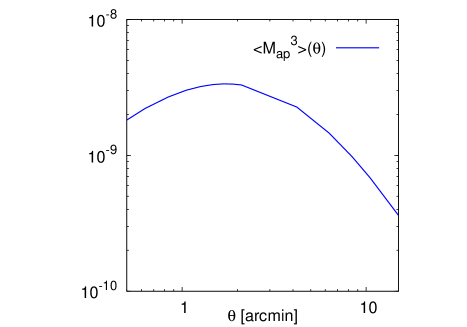
Figure 3: Prediction of the third-order moment of the aperture mass Map3delimited-⟨⟩subscriptsuperscript𝑀3ap\langle M^{3}_{\rm ap}\rangle for sources at redshift zs=0.4subscript𝑧s0.4z_{\rm s}=0.4.

Another conceivable systematic effect is through cosmic magnification (Narayan, 1989; Bartelmann & Schneider, 2001) that is generated by matter density fluctuations in front of lenses. To lowest order, foreground matter density fluctuations with lensing convergence κ<subscript𝜅\kappa_{<} (Eq. 1) integrated to the lens distance modify the observed clustering of lenses on the sky above a certain flux limit flimsubscript𝑓limf_{\rm lim} according to

κg=κg+λκ<+𝒪(κ<2),subscriptsuperscript𝜅gsubscript𝜅g𝜆subscript𝜅𝒪superscriptsubscript𝜅2\kappa^{\prime}_{\rm g}=\kappa_{\rm g}+\lambda\kappa_{<}+{\cal O}(\kappa_{<}^{2})\;, (32)

compared to the unmagnified lens number density κgsubscript𝜅g\kappa_{\rm g}. Here, we have λ:=2(ν1)assign𝜆2𝜈1\lambda:=2(\nu-1) with n¯g(>flim)flimνproportional-toannotatedsubscript¯𝑛gabsentsubscript𝑓limsuperscriptsubscript𝑓lim𝜈\bar{n}_{\rm g}(>f_{\rm lim})\propto f_{\rm lim}^{-\nu} being the mean number density of lenses with flux greater than flimsubscript𝑓limf_{\rm lim}. Normally ν1𝜈1\nu-1 is of the order of unity (van Waerbeke, 2010) or smaller. Likewise the shear distortion γ=γ<+γ>𝛾subscript𝛾subscript𝛾\gamma=\gamma_{<}+\gamma_{>}, Eq. (3), into the same l.o.s. direction contains a contribution γ<subscript𝛾\gamma_{<} related to κ<subscript𝜅\kappa_{<}, and γ>subscript𝛾\gamma_{>} that is the shear originating from matter fluctuations beyond the foreground. This in combination produces as additional contribution to 𝒢=κg,1κg,2(γ<+γ>)𝒢delimited-⟨⟩subscriptsuperscript𝜅g1subscriptsuperscript𝜅g2subscript𝛾subscript𝛾{\cal G}=\langle\kappa^{\prime}_{{\rm g},1}\kappa^{\prime}_{{\rm g},2}(\gamma_{<}+\gamma_{>})\rangle the term λ2κ<,1κ<,2γ<superscript𝜆2delimited-⟨⟩subscript𝜅1subscript𝜅2subscript𝛾\lambda^{2}\langle\kappa_{<,1}\kappa_{<,2}\gamma_{<}\rangle and to G±=κg(γ<,1+γ>,1)(γ<,2+γ>,2)subscript𝐺plus-or-minusdelimited-⟨⟩subscriptsuperscript𝜅gsubscript𝛾1subscript𝛾1subscript𝛾2subscript𝛾2G_{\pm}=\langle\kappa^{\prime}_{\rm g}(\gamma_{<,1}+\gamma_{>,1})(\gamma_{<,2}+\gamma_{>,2})\rangle the term λκ<γ<,1γ<,2𝜆delimited-⟨⟩subscript𝜅subscript𝛾1subscript𝛾2\lambda\langle\kappa_{<}\gamma_{<,1}\gamma_{<,2}\rangle.

These terms are basically third-order cosmic shear correlations or, in terms of the aperture statistics, related to the Map3(θ)delimited-⟨⟩superscriptsubscript𝑀ap3𝜃\langle M_{\rm ap}^{3}(\theta)\rangle statistics (Schneider et al., 2005). Third-order shear correlations have been measured (Bernardeau et al., 2003; Pen et al., 2003; Jarvis et al., 2004; Semboloni et al., 2011), and Map3(θ)delimited-⟨⟩superscriptsubscript𝑀ap3𝜃\langle M_{\rm ap}^{3}(\theta)\rangle has been found (Jarvis et al., 2004; Semboloni et al., 2011) to be of the order of 107less-than-or-similar-toabsentsuperscript107\lesssim 10^{-7} for aperture scales of θ1similar-to𝜃superscript1\theta\sim 1^{\prime} and sources at zs1.0similar-tosubscript𝑧s1.0z_{\rm s}\sim 1.0. As this includes contributions from the entire integrated matter up to zssubscript𝑧sz_{\rm s}, whereas the G3L magnification effect only contributions from the matter integrated up to the lens redshifts zd0.4similar-tosubscript𝑧d0.4z_{\rm d}\sim 0.4, we consider this an empirical upper limit for the magnification effect. In Fig. 3, we show a prediction of Map3(θ)delimited-⟨⟩subscriptsuperscript𝑀3ap𝜃\langle M^{3}_{\rm ap}(\theta)\rangle with sources at zs=0.4subscript𝑧s0.4z_{\rm s}=0.4 for a WMAP7-like cosmology based on the theory described in Semboloni et al. (2011). This result implies that the impact of lens magnification on the G3L aperture statistics is smaller than 108less-than-or-similar-toabsentsuperscript108\lesssim 10^{-8}.

3 Data

Refer to caption
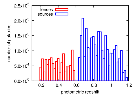
Figure 4: Total number of lenses (red) and sources (blue) in the catalogue between 0.2zphoto<1.20.2subscript𝑧photo1.20.2\leq z_{\rm photo}<1.2 and 17.5i<22.517.5superscript𝑖22.517.5\leq i^{\prime}<22.5 for lenses or 17.5i<24.717.5superscript𝑖24.717.5\leq i^{\prime}<24.7 for sources. The figures comprise all galaxies, complying with the selection cuts, contained within all 172 pointings. For the G3L analysis, the lens sample is further subdivided in luminosity, stellar mass bins and photometric redshift, while sources are rejected for a photo-z𝑧z of zphoto<0.65subscript𝑧photo0.65z_{\rm photo}<0.65.
Table 1: Selection criteria of lens samples and source sample for the G3L analysis applied to the samples in Fig. 4, following Mandelbaum et al. (2006) for the lenses. The luminosity bins (L), stellar mass bins (sm) and galaxy type bins (ETG: early-type galaxies; LTG: late-type galaxies) are again subdivided by 0.2zphoto<0.440.2subscript𝑧photo0.440.2\leq z_{\rm photo}<0.44 (“low-z𝑧z”) and 0.44zphoto<0.60.44subscript𝑧photo0.60.44\leq z_{\rm photo}<0.6 (“high-z𝑧z”). Sources attributed no statistical weight w𝑤w by lensfit are not used in the source sample. The galaxy numbers are for all pointings of which the final analysis discards roughly 25%. Luminosities and stellar masses assume h=0.730.73h=0.73. (1) z¯¯𝑧\bar{z}: mean redshift, σzsubscript𝜎𝑧\sigma_{z}: r.m.s. variance of p(z)𝑝𝑧p(z); (2) and (3): best-fit parameters of ω(θ)=Aω(θ/1)λ+IC𝜔𝜃subscript𝐴𝜔superscript𝜃superscript1𝜆IC\omega(\theta)=A_{\omega}(\theta/1^{\prime})^{-\lambda}+\rm IC within 0.2θ<10superscript0.2𝜃superscript100^{\prime}\!.2\leq\theta<10^{\prime}; (4): sample completeness; (5): mean r𝑟r-band luminosity; (6): mean stellar mass in units of 1010Msuperscript1010subscript𝑀direct-product10^{10}\,M_{\odot}.
Sample Selection #Galaxies z¯±σz(1)plus-or-minus¯𝑧superscriptsubscript𝜎𝑧1\bar{z}\pm\sigma_{z}^{(1)} Aω/0.1(2)subscript𝐴𝜔superscript0.12A_{\omega}/0.1^{(2)} λ(3)superscript𝜆3\lambda^{(3)} fc(4)superscriptsubscript𝑓𝑐4f_{c}^{(4)} Mr(5)superscriptdelimited-⟨⟩subscript𝑀𝑟5\langle M_{r}\rangle^{(5)} M(6)superscriptdelimited-⟨⟩subscript𝑀6\langle M_{\ast}\rangle^{(6)}
L1 low-z𝑧z 18Mr<1718subscript𝑀𝑟17-18\leq M_{r}<-17 36,372 0.22±0.16plus-or-minus0.220.160.22\pm 0.16 2.40±0.29plus-or-minus2.400.292.40\pm 0.29 0.45±0.11plus-or-minus0.450.110.45\pm 0.11 0.140.140.14 -17.75 0.04
L1 high-z𝑧z
L2 low-z𝑧z 19Mr<1819subscript𝑀𝑟18-19\leq M_{r}<-18 157,306 0.28±0.15plus-or-minus0.280.150.28\pm 0.15 1.91±0.23plus-or-minus1.910.231.91\pm 0.23 0.35±0.05plus-or-minus0.350.050.35\pm 0.05 0.450.450.45 -18.60 0.10
L2 high-z𝑧z
L3 low-z𝑧z 20Mr<1920subscript𝑀𝑟19-20\leq M_{r}<-19 220,329 0.34±0.14plus-or-minus0.340.140.34\pm 0.14 1.41±0.12plus-or-minus1.410.121.41\pm 0.12 0.43±0.05plus-or-minus0.430.050.43\pm 0.05 0.810.810.81 -19.52 0.26
L3 high-z𝑧z 75,902 0.48±0.11plus-or-minus0.480.110.48\pm 0.11 1.63±0.18plus-or-minus1.630.181.63\pm 0.18 0.54±0.08plus-or-minus0.540.080.54\pm 0.08 0.420.420.42 -19.72 0.29
L4 low-z𝑧z 21Mr<2021subscript𝑀𝑟20-21\leq M_{r}<-20 149,190 0.34±0.12plus-or-minus0.340.120.34\pm 0.12 1.63±0.07plus-or-minus1.630.071.63\pm 0.07 0.53±0.03plus-or-minus0.530.030.53\pm 0.03 0.950.950.95 -20.50 0.91
L4 high-z𝑧z 185,286 0.51±0.10plus-or-minus0.510.100.51\pm 0.10 1.62±0.08plus-or-minus1.620.081.62\pm 0.08 0.69±0.04plus-or-minus0.690.040.69\pm 0.04 0.820.820.82 -20.53 0.98
L5 low-z𝑧z 22Mr<2122subscript𝑀𝑟21-22\leq M_{r}<-21 88,916 0.34±0.11plus-or-minus0.340.110.34\pm 0.11 2.19±0.14plus-or-minus2.190.142.19\pm 0.14 0.60±0.05plus-or-minus0.600.050.60\pm 0.05 0.980.980.98 -21.48 3.09
L5 high-z𝑧z 134,369 0.51±0.09plus-or-minus0.510.090.51\pm 0.09 2.06±0.05plus-or-minus2.060.052.06\pm 0.05 0.74±0.02plus-or-minus0.740.020.74\pm 0.02 0.990.990.99 -21.49 3.06
L6 low-z𝑧z 23Mr<2223subscript𝑀𝑟22-23\leq M_{r}<-22 31,373 0.35±0.10plus-or-minus0.350.100.35\pm 0.10 3.02±0.24plus-or-minus3.020.243.02\pm 0.24 0.65±0.07plus-or-minus0.650.070.65\pm 0.07 0.990.990.99 -22.40 8.56
L6 high-z𝑧z 55,315 0.52±0.08plus-or-minus0.520.080.52\pm 0.08 2.50±0.10plus-or-minus2.500.102.50\pm 0.10 0.92±0.04plus-or-minus0.920.040.92\pm 0.04 1.001.001.00 -22.42 8.11
sm1 low-z𝑧z 0.5M/1010M<1.00.5subscript𝑀superscript1010subscript𝑀direct-product1.00.5\leq M_{\ast}/10^{10}M_{\odot}<1.0 78,181 0.34±0.12plus-or-minus0.340.120.34\pm 0.12 2.41±0.34plus-or-minus2.410.342.41\pm 0.34 0.43±0.09plus-or-minus0.430.090.43\pm 0.09 0.940.940.94 -20.49 0.71
sm1 high-z𝑧z 69,784 0.50±0.10plus-or-minus0.500.100.50\pm 0.10 1.72±0.33plus-or-minus1.720.331.72\pm 0.33 0.58±0.15plus-or-minus0.580.150.58\pm 0.15 0.770.770.77 -20.66 0.73
sm2 low-z𝑧z 1.0M/1010M<2.01.0subscript𝑀superscript1010subscript𝑀direct-product2.01.0\leq M_{\ast}/10^{10}M_{\odot}<2.0 61,650 0.34±0.11plus-or-minus0.340.110.34\pm 0.11 3.75±0.82plus-or-minus3.750.823.75\pm 0.82 0.36±0.11plus-or-minus0.360.110.36\pm 0.11 0.980.980.98 -20.98 1.42
sm2 high-z𝑧z 82,411 0.51±0.09plus-or-minus0.510.090.51\pm 0.09 2.39±0.07plus-or-minus2.390.072.39\pm 0.07 0.60±0.07plus-or-minus0.600.070.60\pm 0.07 0.900.900.90 -20.99 1.45
sm3 low-z𝑧z 2.0M/1010M<4.02.0subscript𝑀superscript1010subscript𝑀direct-product4.02.0\leq M_{\ast}/10^{10}M_{\odot}<4.0 48,632 0.34±0.10plus-or-minus0.340.100.34\pm 0.10 3.47±0.31plus-or-minus3.470.313.47\pm 0.31 0.51±0.07plus-or-minus0.510.070.51\pm 0.07 0.990.990.99 -21.46 2.85
sm3 high-z𝑧z 81,305 0.51±0.08plus-or-minus0.510.080.51\pm 0.08 2.44±0.13plus-or-minus2.440.132.44\pm 0.13 0.72±0.05plus-or-minus0.720.050.72\pm 0.05 0.980.980.98 -21.45 2.85
sm4 low-z𝑧z 4.0M/1010M<8.04.0subscript𝑀superscript1010subscript𝑀direct-product8.04.0\leq M_{\ast}/10^{10}M_{\odot}<8.0 33,218 0.35±0.09plus-or-minus0.350.090.35\pm 0.09 4.05±0.39plus-or-minus4.050.394.05\pm 0.39 0.59±0.08plus-or-minus0.590.080.59\pm 0.08 0.990.990.99 -21.91 5.60
sm4 high-z𝑧z 57,049 0.51±0.08plus-or-minus0.510.080.51\pm 0.08 2.72±0.11plus-or-minus2.720.112.72\pm 0.11 0.77±0.04plus-or-minus0.770.040.77\pm 0.04 0.990.990.99 -22.00 5.59
sm5 low-z𝑧z 8.0M/1010M<16.08.0subscript𝑀superscript1010subscript𝑀direct-product16.08.0\leq M_{\ast}/10^{10}M_{\odot}<16.0 15,527 0.36±0.08plus-or-minus0.360.080.36\pm 0.08 5.00±0.41plus-or-minus5.000.415.00\pm 0.41 0.70±0.07plus-or-minus0.700.070.70\pm 0.07 1.001.001.00 -22.40 10.86
sm5 high-z𝑧z 27,598 0.51±0.08plus-or-minus0.510.080.51\pm 0.08 3.56±0.24plus-or-minus3.560.243.56\pm 0.24 0.81±0.07plus-or-minus0.810.070.81\pm 0.07 1.001.001.00 -22.81 10.88
sm6 low-z𝑧z 16.0M/1010M<32.016.0subscript𝑀superscript1010subscript𝑀direct-product32.016.0\leq M_{\ast}/10^{10}M_{\odot}<32.0 4,605 0.36±0.07plus-or-minus0.360.070.36\pm 0.07 6.58±0.50plus-or-minus6.580.506.58\pm 0.50 1.51±0.07plus-or-minus1.510.071.51\pm 0.07 1.001.001.00 -23.00 21.13
sm6 high-z𝑧z 7,121 0.52±0.07plus-or-minus0.520.070.52\pm 0.07 4.18±0.78plus-or-minus4.180.784.18\pm 0.78 1.58±0.16plus-or-minus1.580.161.58\pm 0.16 1.001.001.00 -23.22 20.90
sm7 low-z𝑧z 32.0M/1010M<64.032.0subscript𝑀superscript1010subscript𝑀direct-product64.032.0\leq M_{\ast}/10^{10}M_{\odot}<64.0 526 0.38±0.06plus-or-minus0.380.060.38\pm 0.06 8.89±1.37plus-or-minus8.891.378.89\pm 1.37 1.64±0.15plus-or-minus1.640.151.64\pm 0.15 1.001.001.00 -23.60 40.81
sm7 high-z𝑧z 775 0.52±0.07plus-or-minus0.520.070.52\pm 0.07 5.61±1.30plus-or-minus5.611.305.61\pm 1.30 1.28±0.21plus-or-minus1.280.211.28\pm 0.21 1.001.001.00 -23.67 38.52
ETG low-z𝑧z 00absent0\leqT_B<2|23Mr<21bra223subscript𝑀𝑟21<2~{}|~{}-23\leq M_{r}<-21 89,359 0.34±0.10plus-or-minus0.340.100.34\pm 0.10 3.43±0.08plus-or-minus3.430.083.43\pm 0.08 0.68±0.02plus-or-minus0.680.020.68\pm 0.02 0.990.990.99 -21.88 5.91
ETG high-z𝑧z 137,144 0.51±0.08plus-or-minus0.510.080.51\pm 0.08 2.90±0.09plus-or-minus2.900.092.90\pm 0.09 0.83±0.03plus-or-minus0.830.030.83\pm 0.03 1.001.001.00 -21.91 5.74
LTG low-z𝑧z 22absent2\leqT_B<6|23Mr<21bra623subscript𝑀𝑟21<6~{}|~{}-23\leq M_{r}<-21 30,926 0.35±0.13plus-or-minus0.350.130.35\pm 0.13 0.70±0.13plus-or-minus0.700.130.70\pm 0.13 0.87±0.18plus-or-minus0.870.180.87\pm 0.18 0.960.960.96 -21.64 1.73
LTG high-z𝑧z 52,527 0.51±0.10plus-or-minus0.510.100.51\pm 0.10 1.33±0.16plus-or-minus1.330.161.33\pm 0.16 0.78±0.11plus-or-minus0.780.110.78\pm 0.11 0.990.990.99 -21.73 2.05
SOURCES 0.65zphoto<1.2|w>00.65subscript𝑧photoinner-product1.2𝑤00.65\leq z_{\rm photo}<1.2~{}|~{}w>0 2,926,894 0.93±0.26plus-or-minus0.930.260.93\pm 0.26
Refer to caption
Refer to caption
Refer to caption
Refer to caption
Refer to caption
Refer to caption
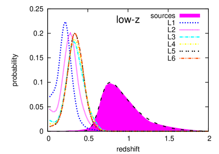
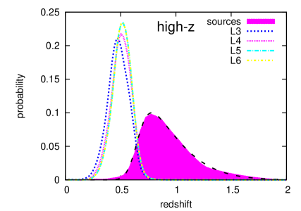
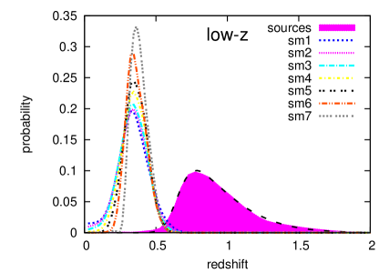
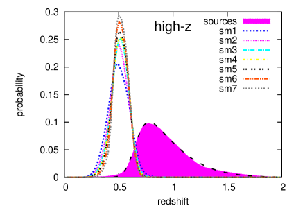
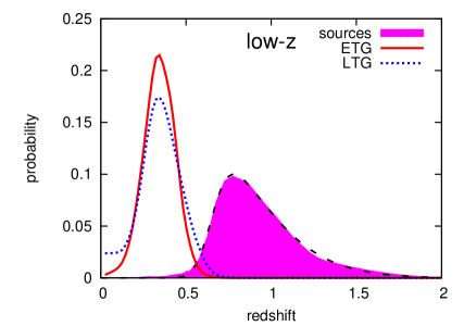
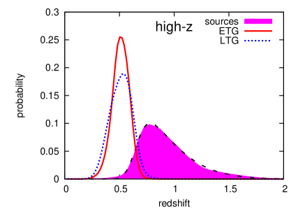
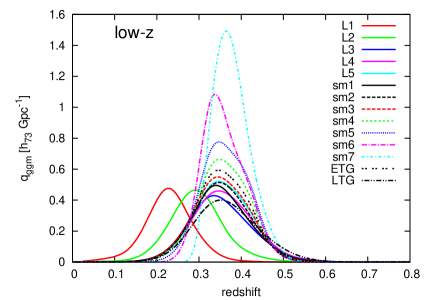
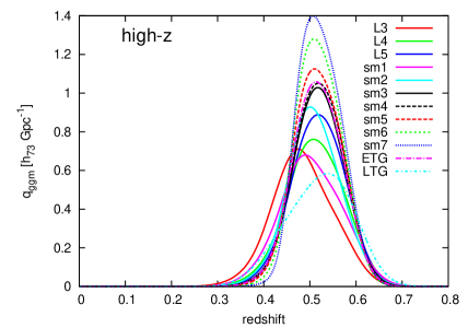
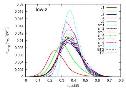
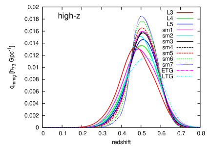
Figure 5: In contrast to Fig. 4, this figure shows the full BPZ redshift posterior of the various samples. Low-z𝑧z lenses are selected from zphoto[0.2,0.44]subscript𝑧photo0.20.44z_{\rm photo}\in[0.2,0.44], high-z𝑧z lenses from zphoto[0.44,0.6]subscript𝑧photo0.440.6z_{\rm photo}\in[0.44,0.6], and sources from zphoto[0.65,1.2]subscript𝑧photo0.651.2z_{\rm photo}\in[0.65,1.2]. The dashed black line enclosing the source p.d.f. is a parametrised fit, see Sect. 3.3 for best-fit parameters.

3.1 Object selection and photometric redshifts

This work uses the full CFHTLenS data set, which originates from the CFHTLS-Wide Survey. The CFHTLS-Wide imaged 171 MegaCam (mounted on the CFHT) pointings in the five broad-band filters usuperscript𝑢u^{*}, gsuperscript𝑔g^{\prime}, rsuperscript𝑟r^{\prime}, isuperscript𝑖i^{\prime}, and zsuperscript𝑧z^{\prime}. During the observation campaign of CFHTLS, the isuperscript𝑖i^{\prime}-band filter was replaced by a new filter with a slightly different transmission curve. For some of the pointings only the updated isuperscript𝑖i^{\prime}-band filter magnitudes are available, which are treated as the old filter magnitudes in the analysis. For details, see Erben et al. (2012).

CFHTLenS has an effective area (different pointings partly overlap) of about 154 square-degrees with high-quality photometric redshifts down to i24.7superscript𝑖24.7i^{\prime}\approx 24.7. The data set and the extraction of our photometric redshift catalogue are described in Hildebrandt et al. (2012). Our data processing techniques and recipes are described in Erben et al. (2009) and Erben et al. (2012). As primary selection criterion, we select sources brighter than i<24.7superscript𝑖24.7i^{\prime}<24.7 and lenses brighter than i<22.5superscript𝑖22.5i^{\prime}<22.5. This will be further subdivided in the following by using photometric redshifts (Fig. 4) and, in the case of lenses, Mrsubscript𝑀𝑟M_{r} rest frame magnitudes, stellar masses or SED information (details below). 43 pointings out of 171 exhibit a significant PSF residual signal, according to the detailed tests in Sect. 4.2 of Heymans et al. (2012), and are therefore discarded for the analysis (25%similar-toabsentpercent25\sim 25\% area); 129 pointings are included in the analysis. This leaves a total effective survey area of 120deg2similar-toabsent120superscriptdeg2\sim 120\,\rm deg^{2} that is eventually used in the analysis. Of this area an additional 20%similar-toabsentpercent20\sim 20\% percent is lost due to masking. The analysis is performed on individual fields which allows us to use field-to-field variances of the measurements to estimate the covariance of measurement errors directly from the data.

3.2 Lens samples

To guarantee a high reliability of the photo-z𝑧z estimates for the lenses, a magnitude cut of i22.5superscript𝑖22.5i^{\prime}\leq 22.5 is applied. A detailed account and tests of the CFHTLenS photo-z𝑧z pipeline can be found in Hildebrandt et al. (2012). Based on the galaxies endowed with photometric redshifts, three classes of lens samples are selected (Table 1):

  • A luminosity or L-sample class, which consists of six distinct rest-frame Mrsubscript𝑀𝑟M_{r} bins (SDSS r𝑟r-filter; York et al., 2000), labelled L1 to L6. The same formal luminosity bin limits as in Mandelbaum et al. (2006) or Velander et al. (2012) are applied, although we do not automatically expect equivalent completeness of the samples. To quantify the completeness, we introduce the fcsubscript𝑓cf_{\rm c} parameter below.

  • A stellar mass or sm-sample class, which is also further subdivided using seven distinct stellar mass bins. Again, we are guided by Mandelbaum et al. (2006) for compiling this sample class. The sm class has sub-classes with labels sm1-sm7.

  • A galaxy type class using the T_B parameter in BPZ (Benitez, 2000), which provides the most likely galaxy SED for a given galaxy and its estimated photo-z𝑧z; see Erben et al. (2012) for more details. T_B=2 as division line, we separate early-type galaxies (“ETG”), which have T_B<2absent2<2, from late type galaxies (“LTG”).111Within BPZ values of T_B denote best-fitting galaxy templates: 1=CWW-Ell, 2=CWW-Sbc, 3=CWW-Scd, 4=CWW-Im, 5=KIN-SB3, and 6=KIN-SB2. Note that the templates are interpolated, such that fractional numbers occur. In order to define a volume-limited sample of ETG and LTG, we select only luminous galaxies with restframe luminosities 23Mr<2123subscript𝑀𝑟21-23\leq M_{r}<-21. With this luminosity cut, ETG and LTG are actually subsamples of L5 and L6 combined.

The stellar masses of the lenses are determined from the galaxy multi-colour data as described in Sect. 2.1 of Velander et al. (2012). The estimators assume a Chabrier (2003) star initial mass function.

All three classes are further split into two photo-z𝑧z bins: a “low-z𝑧z” bin with 0.2zphoto<0.440.2subscript𝑧photo0.440.2\leq z_{\rm photo}<0.44 and a “high-z𝑧z” bin with 0.44zphoto<0.600.44subscript𝑧photo0.600.44\leq z_{\rm photo}<0.60. As redshift estimators we use the maximum probability redshifts of the redshift posterior provided by BPZ. The redshift boundaries give comparable numbers of lenses prior to attributing them to one of the three lens classes (Fig. 4). Not counting the high-z𝑧z L1 and L2 samples, which have too faint limits to contain lenses222Actually, we find a few galaxies in the high-z𝑧z L1/L2 samples. These are probably extreme outliers with greatly inaccurate redshift estimates., we have in total 28 lens subsamples.

The true redshift distribution of a lens sample is not identical to the distribution of their photometric redshifts due to the errors in the photo-z𝑧z estimators. For a magnitude cut of i<22.5superscript𝑖22.5i^{\prime}<22.5, the errors are approximately σz0.04(1+z)less-than-or-similar-tosubscript𝜎z0.041𝑧\sigma_{\rm z}\lesssim 0.04(1+z) with a 3%similar-toabsentpercent3\sim 3\% outlier rate (Hildebrandt et al., 2012). We combine the posterior redshift probability distribution functions (p.d.f.) of all lenses given by BPZ, see Fig. 5, to quantify the redshift uncertainties of complete lens samples. The depicted redshift probability distributions will be utilised when normalising the G3L aperture statistics.

To help the comparison of our G3L results to future studies, we also quote the angular clustering and completeness of the lens samples. The results are listed in Table 1, the details are described in Appendices B.1 (clustering) and B.2 (completeness). In short, for the angular clustering of lenses, we approximate the angular galaxy two-point correlation function by a power law over the angular range 0.2θ<10superscript0.2𝜃superscript100^{\prime}\!\!.2\leq\theta<10^{\prime}. For each lens sample with the photo-z𝑧z bin [z1,z2]subscript𝑧1subscript𝑧2[z_{1},z_{2}], we quote the completeness factor fcsubscript𝑓cf_{\rm c} that expresses the average V(z1,zmax)/V(z1,z2)𝑉subscript𝑧1subscript𝑧max𝑉subscript𝑧1subscript𝑧2V(z_{1},z_{\rm max})/V(z_{1},z_{2}) of all lenses in the sample; V(z1,z2)𝑉subscript𝑧1subscript𝑧2V(z_{1},z_{2}) is the light cone volume between redshift z1subscript𝑧1z_{1} and z2subscript𝑧2z_{2}, and zmaxz2subscript𝑧maxsubscript𝑧2z_{\rm max}\leq z_{2} is the maximum redshift up to which a lens is still above the flux limit i=22.5superscript𝑖22.5i^{\prime}=22.5. A small fcsubscript𝑓cf_{\rm c} is a sign of a strong incompleteness because many galaxies similar to those observed near z1subscript𝑧1z_{1} are presumably missing at higher redshifts. Due to the magnitude limit, samples containing a substantial portion of faint galaxies are most affected by incompleteness, most notably L1 and L2. As expected, the completeness drops if one moves from the low-z𝑧z to the high-z𝑧z bin in almost all cases. The few minor exceptions, L5 for instance, are probably due to shot noise in the fcsubscript𝑓cf_{\rm c} estimator. We conclude that L4-L6, sm3-sm7 and ETG/LTG are the most complete, volume-limited samples for our study (fc>0.80subscript𝑓c0.80f_{\rm c}>0.80 for both low-z𝑧z and high-z𝑧z). In Table 1 we also quote the average absolute r𝑟r-band flux of the samples, listed as magnitude Mrdelimited-⟨⟩subscript𝑀𝑟\langle M_{r}\rangle and the their average stellar mass Mdelimited-⟨⟩subscript𝑀\langle M_{\ast}\rangle.

3.3 Source sample

All details concerning the galaxy shape measurement (employing the lensfit algorithm; Kitching et al. 2008, Miller et al. 2007, and Miller et al. 2012), CFHTLenS source catalogue generation, and the discussion of shear systematics are presented in Heymans et al. (2012) and Miller et al. (2012). We account for the multiplicative shear bias by employing the Miller et al. (2012) normalisation scheme adjusted to our estimators (see Appendix A).

In order to reduce the level of undesired II- and GI-correlations in the measurements, we attempt to separate sources and lenses by redshift, utilising photometric redshifts as estimators. As a compromise between accurate redshift estimates and a large numbers of sources, we apply a magnitude limit i<24.7superscript𝑖24.7i^{\prime}<24.7 to the lensfit shear catalogue and select sources between 0.65zphoto<1.20.65subscript𝑧photo1.20.65\leq z_{\rm photo}<1.2. As for the lenses, the true redshift distribution is derived from the combined posterior redshift p.d.f. of individual sources, shown in every panel of Fig. 5 in comparison to the redshift distribution of the lens samples. The individual posteriors are weighted with the source weight that is also used in the lensing analysis. The source redshift p.d.f. is well fitted by a broken exponential distribution

pb(z){exp(p0(z0z)p1)ifzz0,exp(p2(zz0)p3)otherwiseproportional-tosubscript𝑝b𝑧casessubscript𝑝0superscriptsubscript𝑧0𝑧subscript𝑝1if𝑧subscript𝑧0subscript𝑝2superscript𝑧subscript𝑧0subscript𝑝3otherwisep_{\rm b}(z)\propto\left\{\begin{array}[]{ll}\exp{(-p_{0}(z_{0}-z)^{p_{1}})}&{\rm if}~{}z\leq z_{0},\\ \exp{(-p_{2}(z-z_{0})^{p_{3}})}&{\rm otherwise}\end{array}\right. (33)

with fit parameters p0=91.14subscript𝑝091.14p_{0}=91.14, p1=2.623subscript𝑝12.623p_{1}=2.623, p2=4.093subscript𝑝24.093p_{2}=4.093, p3=1.378subscript𝑝31.378p_{3}=1.378 and z0=0.794subscript𝑧00.794z_{0}=0.794 (dashed black lines). With our selections we find about 3×1063superscript1063\times 10^{6} sources with mean redshift z¯0.93¯𝑧0.93\bar{z}\approx 0.93. As can be seen in Fig. 5, the overlap of the various pf(z)subscript𝑝f𝑧p_{\rm f}(z) and the source pb(z)subscript𝑝b𝑧p_{\rm b}(z) is small but not entirely vanishing, mainly at z=0.50.7𝑧0.50.7z=0.5-0.7 for the high-z𝑧z and at z0.6similar-to𝑧0.6z\sim 0.6 for the low-z𝑧z samples. The typical overlapping area of the redshift probability distribution functions (visible in Fig. 5) is 12%similar-toabsentpercent12\sim 12\% for the high-z𝑧z samples and 4%similar-toabsentpercent4\sim 4\% for the low-z𝑧z samples.

4 Results

4.1 Measurements and their uncertainties

In order to obtain measurements for the lensing aperture statistics, we use the method outlined in Sect. 2.3. As the binning grid for 𝒢~estsuperscript~𝒢est\widetilde{\cal G}^{\rm est} and G~±estsuperscriptsubscript~𝐺plus-or-minusest\widetilde{G}_{\pm}^{\rm est}, 100100100 log-bins ranging between 9 arcsec and 50 arcmin are set up for ϑ1/2subscriptitalic-ϑ12\vartheta_{1/2}, 100100100 linear bins are used for the opening angle ϕ3subscriptitalic-ϕ3\phi_{3}, yielding overall 106superscript10610^{6} bins with bin widths Δϕ3=3.6degΔsubscriptitalic-ϕ33.6deg\Delta\phi_{3}=3.6\,\rm deg and Δlnϑ=0.058Δitalic-ϑ0.058\Delta\ln{\vartheta}=0.058. All measurements are performed separately on every individual pointing, out of 129 square pointings with roughly 1deg21superscriptdeg21\,\rm deg^{2} each. Adjacent pointings partly overlap, however, which reduces the area that is actually used. In our study, we crop the pointings to remove the overlap. For the final result, individual estimates are combined by averaging the individual 𝒢~estsuperscript~𝒢est\widetilde{\cal G}^{\rm est} and G~±estsuperscriptsubscript~𝐺plus-or-minusest\widetilde{G}_{\pm}^{\rm est} weighted by the number of triangles within each bin.

Finally, the combined estimates are transformed to the aperture statistics by the integral transformations discussed in SW05. In his way, the aperture statistics between 0.5θap10superscript0.5subscript𝜃apsuperscript100^{\prime}\!\!.5\leq\theta_{\rm ap}\leq 10^{\prime} for ten aperture scale radii are computed. As addressed in Simon et al. (2008), the transformation from 𝒢~~𝒢\tilde{\cal G} or G~±subscript~𝐺plus-or-minus\tilde{G}_{\pm} to aperture statistics becomes biased towards small and large aperture radii due to an insufficient sampling of the correlation functions. A similar transformation bias is also known for the aperture mass statistics (Kilbinger et al., 2006). For the small separations, the bias depends in detail on the mean number density of the galaxies, most crucially the lenses, and the clustering of the lenses, which in combination determines the sampling of the correlation functions by small triangles. By comparison to simulated data, we made sure that this bias is negligible (below 10%similar-toabsentpercent10\sim 10\%) within the range of 1θ10less-than-or-similar-tosuperscript1𝜃less-than-or-similar-tosuperscript101^{\prime}\lesssim\theta\lesssim 10^{\prime} in our case (see Fig. 1 in Saghiha et al. 2012 for an illustration of the transformation bias). The variance of the measurements across all 129 pointings is used to estimate the covariance of measurement errors (Jackknifing; Appendix B.1). The inverse covariance matrix is estimated from the pointing-to-pointing covariance according to the method in Hartlap et al. (2007).
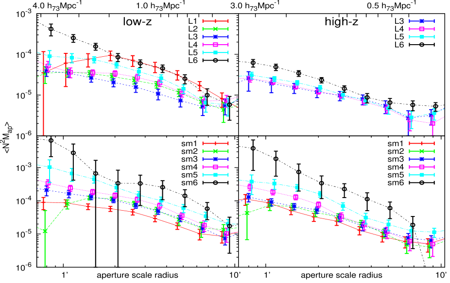
Refer to caption
Refer to caption
Figure 6: Measurements of the E-mode aperture statistics 𝒩2Map(θ)delimited-⟨⟩superscript𝒩2subscript𝑀ap𝜃\langle{\cal N}^{2}M_{\rm ap}\rangle(\theta) (top figure) and 𝒩Map2(θ)delimited-⟨⟩𝒩subscriptsuperscript𝑀2ap𝜃\langle{\cal N}M^{2}_{\rm ap}\rangle(\theta) (bottom figure) as a function of aperture scale radius θ𝜃\theta. The left column depicts measurements for the low-z𝑧z bin, the right column the high-z𝑧z bin. Different lines refer to different lens samples (Table 1). Note that the values get biased for θ1less-than-or-similar-to𝜃superscript1\theta\lesssim 1^{\prime} due to the transformation bias. Error bars indicate the 1σ1𝜎1\sigma standard deviation of the mean of all pointings considered. Missing data points are outside the plotting range but consistent with zero. Numbers at the top indicate the effective scale of the statistics according to the maximum in the u𝑢u-filter. L1-L6: Mrsubscript𝑀𝑟M_{r}-luminosities increasing from -17.8 mag to -22.4 mag; sm1-sm6: increasing stellar masses from 7×10⁹M7superscript109subscript𝑀direct-product7\times 10^{9}\,M_{\odot} to 2×10¹¹M2superscript1011subscript𝑀direct-product2\times 10^{11}\,M_{\odot}.
Refer to caption
Figure 7: Aperture statistics results for the late-type and early-type lens samples. The left column shows the low-z𝑧z redshift bin, the right column the high-z𝑧z redshift bin. Top row and bottom row correspond to 𝒩2Mapdelimited-⟨⟩superscript𝒩2subscript𝑀ap\langle{\cal N}^{2}M_{\rm ap}\rangle and 𝒩Map2delimited-⟨⟩𝒩subscriptsuperscript𝑀2ap\langle{\cal N}M^{2}_{\rm ap}\rangle, respectively. Numbers at the top indicate the effective scale according to the maximum in the u𝑢u-filter. ETG: early-type galaxies; LTG: late-type galaxies.
Table 2: Results of the null tests for the different channels of the statistics. Quoted values are the reduced Δχ2Δsuperscript𝜒2\Delta\chi^{2} with d.o.f=7. for the E-modes and P-mode, 𝒩2Mdelimited-⟨⟩superscript𝒩2subscript𝑀perpendicular-to\langle{\cal N}^{2}M_{\perp}\rangle, and d.o.f.=14 for the combined B/P-mode, 𝒩M2delimited-⟨⟩𝒩subscriptsuperscript𝑀2perpendicular-to\langle{\cal N}M^{2}_{\perp}\rangle and 𝒩MMapdelimited-⟨⟩𝒩subscript𝑀perpendicular-tosubscript𝑀ap\langle{\cal N}M_{\perp}M_{\rm ap}\rangle. E-modes consistent with a null signal are in bold, P- or P/B-modes inconsistent with a null signal are underlined. Adopted confidence levels are 95%percent9595\%. Only data points within the range 1.5θ<10superscript1.5𝜃superscript101^{\prime}\!\!.5\leq\theta<10^{\prime} were used for this test.
0.22zphoto<0.440.22subscript𝑧photo0.440.22\leq z_{\rm photo}<0.44 0.44zphoto<0.600.44subscript𝑧photo0.600.44\leq z_{\rm photo}<0.60
𝒩2Mapdelimited-⟨⟩superscript𝒩2subscript𝑀ap\langle{\cal N}^{2}M_{\rm ap}\rangle 𝒩Map2delimited-⟨⟩𝒩subscriptsuperscript𝑀2ap\langle{\cal N}M^{2}_{\rm ap}\rangle 𝒩2Mapdelimited-⟨⟩superscript𝒩2subscript𝑀ap\langle{\cal N}^{2}M_{\rm ap}\rangle 𝒩Map2delimited-⟨⟩𝒩subscriptsuperscript𝑀2ap\langle{\cal N}M^{2}_{\rm ap}\rangle
Sample E-mode P-mode E-mode P/B-mode E-mode P-mode E-mode P/B-mode
L1 3.22 1.27 2.64 1.24
L2 7.32 1.57 2.31 1.75
L3 3.79 0.66 4.93 0.75 3.21 0.94 2.38 1.22
L4 9.26 0.58 2.62 1.14 7.66 0.89 2.38 0.79
L5 6.72 1.00 4.31 0.80 7.08 1.95 0.81 1.06
L6 7.76 0.99 4.92 0.74 7.07 1.50 1.74 0.41
sm1 6.41 1.06 4.06 1.55 5.18 0.74 1.90 0.68
sm2 12.43 0.59 3.55 1.11 5.97 0.40 0.95 0.83
sm3 7.07 0.99 4.05 0.76 5.62 0.65 0.18 1.19
sm4 7.64 1.86 4.83 0.58 5.93 0.27 2.28 1.12
sm5 3.76 1.27 4.95 0.52 6.74 1.18 0.78 0.96
sm6 0.65 0.91 1.15 1.00 2.33 0.68 0.64 1.42
sm7 0.93 1.16 0.66 1.61 0.45 0.42 1.52 1.87
ETG 12.50 0.87 6.62 0.65 15.24 1.74 1.21 1.06
LTG 0.77 0.85 1.58 1.52 0.90 1.20 1.45 0.37

4.2 E-mode measurements

Fig. 6 summarises the E-mode results for the luminosity and stellar mass bins of the 𝒩2Mapdelimited-⟨⟩superscript𝒩2subscript𝑀ap\langle{\cal N}^{2}M_{\rm ap}\rangle (top) and 𝒩Map2delimited-⟨⟩𝒩subscriptsuperscript𝑀2ap\langle{\cal N}M^{2}_{\rm ap}\rangle statistics (bottom). Due to the incompleteness in the samples, L1 and L2 are empty in the higher redshift bin and hence are missing in the corresponding plots. Likewise, due to the small number of lenses and correspondingly large error bars, also the data points of sm7 are missing. The signal dependence on galaxy type is displayed separately in Fig. 7. For aperture radii greater than 2similar-toabsent2\sim 2 arcmin the measurements seem to be well approximated by power laws, which will be determined below. Below roughly 2 arcmin there are indications of deviations from the power-law behaviour at smaller radii in several cases, e.g., 𝒩2Mapdelimited-⟨⟩superscript𝒩2subscript𝑀ap\langle{\cal N}^{2}M_{\rm ap}\rangle of low-z𝑧z L1/L4, or 𝒩Map2delimited-⟨⟩𝒩superscriptsubscript𝑀ap2\langle{\cal N}M_{\rm ap}^{2}\rangle of high-z𝑧z L4/L6.

The result of 𝒩2Mapdelimited-⟨⟩superscript𝒩2subscript𝑀ap\langle{\cal N}^{2}M_{\rm ap}\rangle of the late-type galaxies (LTG) stand out as being the only one that is completely consistent with zero despite relatively small error bars. Therefore, the excess mass around late-type galaxy pairs vanishes within the statistical uncertainties. In strong contrast to that, the corresponding signal of the early-type galaxy (ETG) sample is highly significant. From the LTG signal upper limit we estimate the ETG signal to be greater by a factor of at least 10similar-toabsent10\sim 10. This confirms the prediction of Saghiha et al. (2012) that is based on galaxy population synthesis models.

The low-z𝑧z sample L1, with the fewest number of lenses, presumably is affected by the transformation bias. This can be seen by the clear drop of the data points for 𝒩2Mapdelimited-⟨⟩superscript𝒩2subscript𝑀ap\langle{\cal N}^{2}M_{\rm ap}\rangle below θap2arcminsimilar-tosubscript𝜃ap2arcmin\theta_{\rm ap}\sim 2\,\rm arcmin compared to a power-law behaviour at larger scales.

4.3 Systematics tests

General tests for systematics on the level of shear catalogue generation are to be found in Heymans et al. (2012). We only use CFHTLenS pointings that passed the therein described tests for cosmic shear applications. To further test for systematics in our measurements, we check for the consistency of the aperture statistics B- and P-modes with a null signal. The details of this test and, moreover, G3L measurements within separate CFHTLenS fields (W1-W4) are presented in Appendix C. The null test also allows to quantify the significance of the signal in the E-mode channels of the statistics. Table 2 summarises the tests for all statistics and galaxy samples.

In summary, we find that B/P-modes in the aperture statistics are consistent with zero between 1 arcmin and 10 arcmin. When looking at the combined L1-L6 sample, separate measurements within the survey fields W1-W4 agree well for both the low-z𝑧z and the high-z𝑧z redshift bin. This demonstrates the internal consistency of the data, and that the observed signals do not originate from a single, possibly peculiar field. As to the E-mode channels of the statistics, we find for 𝒩2Mapdelimited-⟨⟩superscript𝒩2subscript𝑀ap\langle{\cal N}^{2}M_{\rm ap}\rangle highly significant signals (95%percent9595\% confidence) for all low-z𝑧z samples, except for sm6 and sm7, and most high-z𝑧z lens samples. Sm6 and sm7 pose exceptions because they contain relatively small numbers of galaxies. Apart from the high-z𝑧z L3, L4, and sm4, all high-z𝑧z sample measurements of 𝒩Map2delimited-⟨⟩𝒩subscriptsuperscript𝑀2ap\langle{\cal N}M^{2}_{\rm ap}\rangle are consistent with zero, whereas their low-z𝑧z counterparts are mostly significant. As 𝒩Map2delimited-⟨⟩𝒩subscriptsuperscript𝑀2ap\langle{\cal N}M^{2}_{\rm ap}\rangle involves a three-point correlation function with two sources and one lens, the noise level of this measurement is naturally higher than for 𝒩2Mapdelimited-⟨⟩superscript𝒩2subscript𝑀ap\langle{\cal N}^{2}M_{\rm ap}\rangle.

5 Interpretation

Refer to caption
Figure 8: Visualisation of the 𝒢𝒢\cal G-measurement. Shown is the excess mass κg(𝜽1)κg(𝜽2)κ(𝜽3)delimited-⟨⟩subscript𝜅gsubscript𝜽1subscript𝜅gsubscript𝜽2𝜅subscript𝜽3\langle\kappa_{\rm g}({\mn@boldsymbol{\theta}}_{1})\kappa_{\rm g}({\mn@boldsymbol{\theta}}_{2})\kappa({\mn@boldsymbol{\theta}}_{3})\rangle (intensity scale) as function of 𝜽3subscript𝜽3{\mn@boldsymbol{\theta}}_{3} around early-type (top) and late-type galaxy pairs (bottom) with mean angular separations |𝜽1𝜽2|subscript𝜽1subscript𝜽2|{\mn@boldsymbol{\theta}}_{1}-{\mn@boldsymbol{\theta}}_{2}| between 40 and 60 arcsec; one map pixel corresponds to 1.67 arcsec (x𝑥x- and y𝑦y-axis labels). The lens positions 𝜽1,𝜽2subscript𝜽1subscript𝜽2{\mn@boldsymbol{\theta}}_{1},{\mn@boldsymbol{\theta}}_{2} are indicated as boxes, the contours show the S/N levels 2,3,232,3,\ldots (positive excess mass) and -3,-2 (negative excess mass). To increase the signal-to-noise the low-z𝑧z and high-z𝑧z maps of the ETG and LTG samples have been combined. A smoothing with a Gaussian kernel of r.m.s.-size 6.76.76.7 arcsec has been applied to map.

5.1 Lens-pair excess mass

Although aperture statistics and G3L-correlators essentially contain the same information, we would like to show our 𝒢𝒢\cal G-measurements for at least the ETG and LTG samples. As outlined in Simon et al. (2008), the G3L correlation function 𝒢𝒢\cal G can conveniently be interpreted as a convergence map (excess mass map) once the separation of the two lenses is fixed; the E-mode in 𝒢𝒢\cal G is a series of such maps for varying lens-lens separations. After a rotation, the correlator 𝒢~~𝒢\widetilde{\cal G} is a stacked shear field around the lens pair, from which we subtract off the GGL signal around individual the lenses to determine the connected part 𝒢𝒢\cal G. To obtain the excess mass maps for the ETG and LTG in Fig. 8 we transform this stacked shear field to a convergence map utilising the algorithm in Kaiser & Squires (1993). For these maps, we consider relatively small lens-lens separations between 40 and 60 arcsec as in Simon et al. (2008), and we combine the maps of the low-z𝑧z and high-z𝑧z samples; lens-lens-source triangles are rescaled inside the map such that lenses are always at the same position in the map (boxes). We also exploit the parity invariance of the maps by averaging the left and right half of the map, thereby increasing the signal-to-noise, see Simon et al. (2008) for details.

The ETG map contains more significant structure and higher convergence values compared to the LTG map, which has only a weak signal. Qualitatively, the excess mass of the ETG sample is concentrated between the lens pair, whereas the LTG lenses seem to possess a small halo of excess mass around the individual lenses and a convergence trough between them. The latter implies that the average convergence about a LTG pair (both lenses at similar distance) at given separation is lower than the sum of convergence around two mean individual late-type galaxies. We will study these maps in more detail in a forthcoming paper and focus on the aperture statistics for the remainder of this paper.
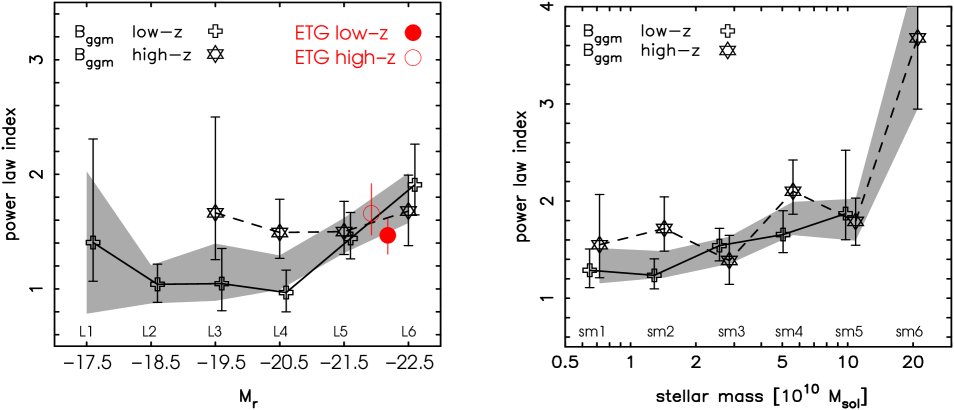
Refer to caption
Figure 9: Dependence of the power-law index α𝛼\alpha in the normalised aperture statistics 𝒩2Mapdelimited-⟨⟩superscript𝒩2subscript𝑀ap\langle{\cal N}^{2}M_{\rm ap}\rangle between 1.5θ<10superscript1.5𝜃superscript101^{\prime}\!\!.5\leq\theta<10^{\prime} with Mrsubscript𝑀𝑟M_{r}-band magnitude (left panel) and stellar mass of lenses (right panel). Table 3 lists the power law indices of all statistics. Only fits to measurements with a 95%percent9595\% confidence detection are plotted. The shaded region highlights the 68%percent6868\% credibility region of the combined low-z𝑧z (open crosses) and high-z𝑧z (open stars). Also shown are the slopes for the early-type galaxy sample in the corresponding magnitude range (left panel). For clarity, these data points are offset about their actual mean Mr=21.88(21.91)delimited-⟨⟩subscript𝑀𝑟21.8821.91\langle M_{r}\rangle=-21.88(-21.91) for the low-z𝑧z (high-z𝑧z) sample.
Table 3: Power-law fits 𝒩nMapm(θ)=A0(θ/1)αdelimited-⟨⟩superscript𝒩𝑛subscriptsuperscript𝑀𝑚ap𝜃subscript𝐴0superscript𝜃superscript1𝛼\langle{\cal N}^{n}M^{m}_{\rm ap}\rangle(\theta)=A_{0}(\theta/1^{\prime})^{-\alpha} to the measured aperture statistics in Fig. 6; A0subscript𝐴0A_{0} is the signal amplitude at an aperture scale radius of θ=1arcmin𝜃1arcmin\theta=1\,\rm arcmin. The fit considers only data within θ[1.5,10]𝜃superscript1.5superscript10\theta\in[1^{\prime}\!\!.5,10^{\prime}]. Quoted errors bracket a 68%percent6868\% credibility region about the median.
0.20zphoto<0.440.20subscript𝑧photo0.440.20\leq z_{\rm photo}<0.44 0.44zphoto<0.600.44subscript𝑧photo0.600.44\leq z_{\rm photo}<0.60
𝒩2Mapdelimited-⟨⟩superscript𝒩2subscript𝑀ap\langle{\cal N}^{2}M_{\rm ap}\rangle 𝒩Map2delimited-⟨⟩𝒩subscriptsuperscript𝑀2ap\langle{\cal N}M^{2}_{\rm ap}\rangle 𝒩2Mapdelimited-⟨⟩superscript𝒩2subscript𝑀ap\langle{\cal N}^{2}M_{\rm ap}\rangle 𝒩Map2delimited-⟨⟩𝒩subscriptsuperscript𝑀2ap\langle{\cal N}M^{2}_{\rm ap}\rangle
Sample A0/105subscript𝐴0superscript105A_{0}/10^{-5} α𝛼\alpha A0/107subscript𝐴0superscript107A_{0}/10^{-7} α𝛼\alpha A0/105subscript𝐴0superscript105A_{0}/10^{-5} α𝛼\alpha A0/107subscript𝐴0superscript107A_{0}/10^{-7} α𝛼\alpha
L1 10.574.90+5.12superscriptsubscript10.574.905.1210.57_{-4.90}^{+5.12} 1.400.34+0.90superscriptsubscript1.400.340.901.40_{-0.34}^{+0.90} 54.3820.06+25.92superscriptsubscript54.3820.0625.9254.38_{-20.06}^{+25.92} 2.590.59+0.94superscriptsubscript2.590.590.942.59_{-0.59}^{+0.94}
L2 5.150.99+1.05superscriptsubscript5.150.991.055.15_{-0.99}^{+1.05} 1.040.16+0.18superscriptsubscript1.040.160.181.04_{-0.16}^{+0.18} 9.4811.37+8.30superscriptsubscript9.4811.378.309.48_{-11.37}^{+8.30} 2.110.73+1.59superscriptsubscript2.110.731.592.11_{-0.73}^{+1.59}
L3 3.660.98+1.04superscriptsubscript3.660.981.043.66_{-0.98}^{+1.04} 1.050.24+0.31superscriptsubscript1.050.240.311.05_{-0.24}^{+0.31} 28.226.63+7.95superscriptsubscript28.226.637.9528.22_{-6.63}^{+7.95} 1.870.29+0.44superscriptsubscript1.870.290.441.87_{-0.29}^{+0.44} 8.562.75+3.78superscriptsubscript8.562.753.788.56_{-2.75}^{+3.78} 1.660.41+0.84superscriptsubscript1.660.410.841.66_{-0.41}^{+0.84} 41.0721.95+27.18superscriptsubscript41.0721.9527.1841.07_{-21.95}^{+27.18} 3.841.06+0.71superscriptsubscript3.841.060.713.84_{-1.06}^{+0.71}
L4 5.100.95+1.04superscriptsubscript5.100.951.045.10_{-0.95}^{+1.04} 0.970.17+0.20superscriptsubscript0.970.170.200.97_{-0.17}^{+0.20} 16.766.88+8.95superscriptsubscript16.766.888.9516.76_{-6.88}^{+8.95} 1.950.51+1.14superscriptsubscript1.950.511.141.95_{-0.51}^{+1.14} 6.851.34+1.50superscriptsubscript6.851.341.506.85_{-1.34}^{+1.50} 1.490.23+0.29superscriptsubscript1.490.230.291.49_{-0.23}^{+0.29} 31.9013.26+18.06superscriptsubscript31.9013.2618.0631.90_{-13.26}^{+18.06} 3.300.87+0.95superscriptsubscript3.300.870.953.30_{-0.87}^{+0.95}
L5 12.302.33+2.47superscriptsubscript12.302.332.4712.30_{-2.33}^{+2.47} 1.440.18+0.23superscriptsubscript1.440.180.231.44_{-0.18}^{+0.23} 34.5610.48+14.41superscriptsubscript34.5610.4814.4134.56_{-10.48}^{+14.41} 1.990.37+0.80superscriptsubscript1.990.370.801.99_{-0.37}^{+0.80} 9.151.70+1.80superscriptsubscript9.151.701.809.15_{-1.70}^{+1.80} 1.500.20+0.26superscriptsubscript1.500.200.261.50_{-0.20}^{+0.26} 8.8918.56+14.23superscriptsubscript8.8918.5614.23-8.89_{-18.56}^{+14.23} 3.581.33+0.88superscriptsubscript3.581.330.883.58_{-1.33}^{+0.88}
L6 35.547.80+9.15superscriptsubscript35.547.809.1535.54_{-7.80}^{+9.15} 1.910.26+0.35superscriptsubscript1.910.260.351.91_{-0.26}^{+0.35} 62.8518.24+25.33superscriptsubscript62.8518.2425.3362.85_{-18.24}^{+25.33} 2.100.36+0.58superscriptsubscript2.100.360.582.10_{-0.36}^{+0.58} 19.895.48+6.28superscriptsubscript19.895.486.2819.89_{-5.48}^{+6.28} 1.680.30+0.31superscriptsubscript1.680.300.311.68_{-0.30}^{+0.31} 42.0721.14+29.43superscriptsubscript42.0721.1429.4342.07_{-21.14}^{+29.43} 3.431.02+0.93superscriptsubscript3.431.020.933.43_{-1.02}^{+0.93}
sm1 11.952.42+2.57superscriptsubscript11.952.422.5711.95_{-2.42}^{+2.57} 1.290.18+0.22superscriptsubscript1.290.180.221.29_{-0.18}^{+0.22} 42.7012.91+19.94superscriptsubscript42.7012.9119.9442.70_{-12.91}^{+19.94} 2.160.46+0.95superscriptsubscript2.160.460.952.16_{-0.46}^{+0.95} 9.342.94+4.01superscriptsubscript9.342.944.019.34_{-2.94}^{+4.01} 1.550.34+0.52superscriptsubscript1.550.340.521.55_{-0.34}^{+0.52} 28.6920.40+28.52superscriptsubscript28.6920.4028.5228.69_{-20.40}^{+28.52} 3.551.26+0.91superscriptsubscript3.551.260.913.55_{-1.26}^{+0.91}
sm2 19.912.96+3.09superscriptsubscript19.912.963.0919.91_{-2.96}^{+3.09} 1.240.14+0.17superscriptsubscript1.240.140.171.24_{-0.14}^{+0.17} 38.1512.24+16.87superscriptsubscript38.1512.2416.8738.15_{-12.24}^{+16.87} 1.900.39+0.82superscriptsubscript1.900.390.821.90_{-0.39}^{+0.82} 14.483.22+3.63superscriptsubscript14.483.223.6314.48_{-3.22}^{+3.63} 1.720.23+0.33superscriptsubscript1.720.230.331.72_{-0.23}^{+0.33} 25.9418.47+22.36superscriptsubscript25.9418.4722.3625.94_{-18.47}^{+22.36} 3.501.08+0.89superscriptsubscript3.501.080.893.50_{-1.08}^{+0.89}
sm3 24.494.91+5.22superscriptsubscript24.494.915.2224.49_{-4.91}^{+5.22} 1.540.16+0.18superscriptsubscript1.540.160.181.54_{-0.16}^{+0.18} 45.0614.01+16.95superscriptsubscript45.0614.0116.9545.06_{-14.01}^{+16.95} 2.090.36+0.85superscriptsubscript2.090.360.852.09_{-0.36}^{+0.85} 11.113.00+3.28superscriptsubscript11.113.003.2811.11_{-3.00}^{+3.28} 1.390.24+0.26superscriptsubscript1.390.240.261.39_{-0.24}^{+0.26} 4.8319.77+16.48superscriptsubscript4.8319.7716.48-4.83_{-19.77}^{+16.48} 3.521.30+0.91superscriptsubscript3.521.300.913.52_{-1.30}^{+0.91}
sm4 34.966.40+6.88superscriptsubscript34.966.406.8834.96_{-6.40}^{+6.88} 1.650.19+0.25superscriptsubscript1.650.190.251.65_{-0.19}^{+0.25} 61.4316.56+19.67superscriptsubscript61.4316.5619.6761.43_{-16.56}^{+19.67} 1.950.29+0.51superscriptsubscript1.950.290.511.95_{-0.29}^{+0.51} 26.165.50+5.84superscriptsubscript26.165.505.8426.16_{-5.50}^{+5.84} 2.100.24+0.32superscriptsubscript2.100.240.322.10_{-0.24}^{+0.32} 31.4616.94+22.60superscriptsubscript31.4616.9422.6031.46_{-16.94}^{+22.60} 3.100.88+1.04superscriptsubscript3.100.881.043.10_{-0.88}^{+1.04}
sm5 87.1925.14+33.76superscriptsubscript87.1925.1433.7687.19_{-25.14}^{+33.76} 1.870.27+0.65superscriptsubscript1.870.270.651.87_{-0.27}^{+0.65} 77.8922.99+26.49superscriptsubscript77.8922.9926.4977.89_{-22.99}^{+26.49} 1.960.29+0.45superscriptsubscript1.960.290.451.96_{-0.29}^{+0.45} 47.3413.26+14.86superscriptsubscript47.3413.2614.8647.34_{-13.26}^{+14.86} 1.790.24+0.24superscriptsubscript1.790.240.241.79_{-0.24}^{+0.24} 63.9335.21+46.24superscriptsubscript63.9335.2146.2463.93_{-35.21}^{+46.24} 3.611.03+0.82superscriptsubscript3.611.030.823.61_{-1.03}^{+0.82}
sm6 197.06347.35+313.36superscriptsubscript197.06347.35313.36197.06_{-347.35}^{+313.36} 3.601.02+0.84superscriptsubscript3.601.020.843.60_{-1.02}^{+0.84} 124.3864.46+83.56superscriptsubscript124.3864.4683.56124.38_{-64.46}^{+83.56} 3.210.91+1.00superscriptsubscript3.210.911.003.21_{-0.91}^{+1.00} 400.32189.83+212.89superscriptsubscript400.32189.83212.89400.32_{-189.83}^{+212.89} 3.680.73+0.72superscriptsubscript3.680.730.723.68_{-0.73}^{+0.72} 53.5168.50+88.69superscriptsubscript53.5168.5088.6953.51_{-68.50}^{+88.69} 3.711.25+0.81superscriptsubscript3.711.250.813.71_{-1.25}^{+0.81}
sm7 315.06274.91+307.91superscriptsubscript315.06274.91307.91315.06_{-274.91}^{+307.91} 3.261.32+1.04superscriptsubscript3.261.321.043.26_{-1.32}^{+1.04} 230.78198.85+265.46superscriptsubscript230.78198.85265.46230.78_{-198.85}^{+265.46} 3.811.19+0.74superscriptsubscript3.811.190.743.81_{-1.19}^{+0.74} 136.21483.19+521.62superscriptsubscript136.21483.19521.62-136.21_{-483.19}^{+521.62} 3.141.15+1.08superscriptsubscript3.141.151.083.14_{-1.15}^{+1.08} 407.91276.37+307.45superscriptsubscript407.91276.37307.45407.91_{-276.37}^{+307.45} 4.091.11+0.57superscriptsubscript4.091.110.574.09_{-1.11}^{+0.57}
ETG 23.272.97+3.05superscriptsubscript23.272.973.0523.27_{-2.97}^{+3.05} 1.490.13+0.16superscriptsubscript1.490.130.161.49_{-0.13}^{+0.16} 41.949.29+10.22superscriptsubscript41.949.2910.2241.94_{-9.29}^{+10.22} 1.710.21+0.29superscriptsubscript1.710.210.291.71_{-0.21}^{+0.29} 21.512.74+2.85superscriptsubscript21.512.742.8521.51_{-2.74}^{+2.85} 1.720.16+0.19superscriptsubscript1.720.160.191.72_{-0.16}^{+0.19} 19.7312.41+16.79superscriptsubscript19.7312.4116.7919.73_{-12.41}^{+16.79} 3.031.03+1.12superscriptsubscript3.031.031.123.03_{-1.03}^{+1.12}
LTG 10.8210.46+13.05superscriptsubscript10.8210.4613.0510.82_{-10.46}^{+13.05} 3.641.16+0.82superscriptsubscript3.641.160.823.64_{-1.16}^{+0.82} 59.4935.02+42.99superscriptsubscript59.4935.0242.9959.49_{-35.02}^{+42.99} 3.861.04+0.70superscriptsubscript3.861.040.703.86_{-1.04}^{+0.70} 3.254.51+5.85superscriptsubscript3.254.515.853.25_{-4.51}^{+5.85} 2.811.52+1.36superscriptsubscript2.811.521.362.81_{-1.52}^{+1.36} 26.8723.95+18.66superscriptsubscript26.8723.9518.66-26.87_{-23.95}^{+18.66} 3.411.19+0.94superscriptsubscript3.411.190.943.41_{-1.19}^{+0.94}

5.2 Power-law fits to measurements

For aperture scale radii larger than θ2greater-than-or-equivalent-to𝜃superscript2\theta\gtrsim 2^{\prime}, our measurements are reasonably consistent with a simple power law. Therefore, we fit power laws 𝒩nMapm(θap)=A0(θ/1)αdelimited-⟨⟩superscript𝒩𝑛superscriptsubscript𝑀ap𝑚subscript𝜃apsubscript𝐴0superscript𝜃superscript1𝛼\langle{\cal N}^{n}M_{\rm ap}^{m}\rangle(\theta_{\rm ap})=A_{0}(\theta/1^{\prime})^{-\alpha} to data points within 1.5θ<10superscript1.5𝜃superscript101^{\prime}\!\!.5\leq\theta<10^{\prime} to quantify the measured profiles of the statistics n=2,m=1formulae-sequence𝑛2𝑚1n=2,m=1 and n=1,m=2formulae-sequence𝑛1𝑚2n=1,m=2, see Table 3. The fit starts at 1.5 arcmin in order not to be too strongly influenced by the transformation bias. Fits use the Jackknife covariance matrices based on the measurements in the different pointings, as in Eq. (48). For the fit, a multivariate Gaussian noise model for the measurement errors is adopted. The quoted values indicate the posterior median and a 68%percent6868\% credibility region about the median for the amplitude A0subscript𝐴0A_{0} and slope α𝛼\alpha. The posterior adopts a top-hat prior for the power-law slope, only allowing values within α[0,5]𝛼05\alpha\in[0,5].

Fig. 9 depicts the dependence of the slope α𝛼\alpha on the lens Mrsubscript𝑀𝑟M_{r} magnitude and stellar mass for 𝒩2Mapdelimited-⟨⟩superscript𝒩2subscript𝑀ap\langle{\cal N}^{2}M_{\rm ap}\rangle of all samples with at least a 95%percent9595\% confidence detection (Table 2). We find a clear trend towards steeper slopes (steeper equilateral bispectra) for more luminous galaxies and galaxies with higher stellar mass. Note that sm6 and sm7 contain on average galaxies more luminous than these of L5 and L6 (Table 1). The figure also depicts the measured slopes for the ETG samples, which are consistent with the L-subsamples of comparable Mrsubscript𝑀𝑟M_{r} luminosity (between L5 and L6). Slopes weakly constrained by the data have posterior medians that are drawn towards the centre of the top-hat prior, α=2.5𝛼2.5\alpha=2.5. This mainly applies to the noisier 𝒩Map2delimited-⟨⟩𝒩subscriptsuperscript𝑀2ap\langle{\cal N}M^{2}_{\rm ap}\rangle measurements, for which reason they are not included in Fig. 9 but are listed in Table 3.

5.3 Normalised measurements

The G3L aperture statistics are directly related to the 3D matter-galaxy cross-bispectra and the redshift distribution of lenses and sources (Sect. 2.4). The radial galaxy distributions and the fiducial cosmology define a smoothing kernel in radial and transverse direction. To disentangle, to lowest order, the dependence of the signal on the physically relevant bispectrum from the dependence on source or lens distribution, we introduce a normalisation scheme.

Combining Eq. (2.4) and Eq. (2.4) shows that 𝒩2Mapdelimited-⟨⟩superscript𝒩2subscript𝑀ap\langle{\cal N}^{2}M_{\rm ap}\rangle constitutes a radially and transversely weighted average of the 3D bispectrum Bggm(𝒌1,𝒌2,χ)subscript𝐵ggmsubscript𝒌1subscript𝒌2𝜒B_{\rm ggm}({\mn@boldsymbol{k}}_{1},{\mn@boldsymbol{k}}_{2},\chi), namely

𝒩2Map(θ1;θ2;θ3)delimited-⟨⟩superscript𝒩2subscript𝑀apsubscript𝜃1subscript𝜃2subscript𝜃3\displaystyle\langle{\cal N}^{2}M_{\rm ap}\rangle(\theta_{1};\theta_{2};\theta_{3})
=3Ωm2DH20χHdχg(χ)pf2(χ)fK3(χ)a2(χ)d21d22d23(2π)6absent3subscriptΩm2superscriptsubscript𝐷H2superscriptsubscript0subscript𝜒Hdifferential-d𝜒𝑔𝜒superscriptsubscript𝑝f2𝜒superscriptsubscript𝑓K3𝜒superscript𝑎2𝜒superscriptd2subscript1superscriptd2subscript2superscriptd2subscript3superscript2𝜋6\displaystyle\!\!\!\!=\frac{3\Omega_{\rm m}}{2D_{\rm H}^{2}}\int_{0}^{\chi_{\rm H}}\!\!\!{\rm d}\chi\frac{g(\chi)p_{\rm f}^{2}(\chi)}{f_{\rm K}^{3}(\chi)a^{2}(\chi)}\int\frac{{\rm d}^{2}\ell_{1}{\rm d}^{2}\ell_{2}{\rm d}^{2}\ell_{3}}{(2\pi)^{6}}
×u~(1θ1)u~(2θ2)u~(3θ3)absent~𝑢subscript1subscript𝜃1~𝑢subscript2subscript𝜃2~𝑢subscript3subscript𝜃3\displaystyle~{}~{}\times\tilde{u}(\ell_{1}\theta_{1})\tilde{u}(\ell_{2}\theta_{2})\tilde{u}(\ell_{3}\theta_{3})
×(2π)2δD(1+2+3)Bggm(1fK(χ),2fK(χ),χ).absentsuperscript2𝜋2subscript𝛿Dsubscriptbold-ℓ1subscriptbold-ℓ2subscriptbold-ℓ3subscript𝐵ggmsubscriptbold-ℓ1subscript𝑓K𝜒subscriptbold-ℓ2subscript𝑓K𝜒𝜒\displaystyle~{}~{}\times(2\pi)^{2}\delta_{\rm D}({\mn@boldsymbol{\ell}}_{1}+{\mn@boldsymbol{\ell}}_{2}+{\mn@boldsymbol{\ell}}_{3})B_{\rm ggm}\big{(}\frac{{\mn@boldsymbol{\ell}}_{1}}{f_{\rm K}(\chi)},\frac{{\mn@boldsymbol{\ell}}_{2}}{f_{\rm K}(\chi)},\chi\big{)}\;.

By changing the integration variables as in i=fK(χ)𝒌isubscriptbold-ℓ𝑖subscript𝑓K𝜒subscript𝒌𝑖{\mn@boldsymbol{\ell}}_{i}=f_{\rm K}(\chi){\mn@boldsymbol{k}}_{i} we write this integral as

𝒩2Map(θ1;θ2;θ3)delimited-⟨⟩superscript𝒩2subscript𝑀apsubscript𝜃1subscript𝜃2subscript𝜃3\displaystyle\langle{\cal N}^{2}M_{\rm ap}\rangle(\theta_{1};\theta_{2};\theta_{3})
=:0χhdχqggm(χ)\displaystyle\!\!\!=:\int_{0}^{\chi_{\rm h}}{\rm d}\chi\,q_{{\rm ggm}}(\chi)
×B¯ggm(1fK(χ)θ1,1fK(χ)θ2,1fK(χ)θ3,χ),absentsubscript¯𝐵ggm1subscript𝑓K𝜒subscript𝜃11subscript𝑓K𝜒subscript𝜃21subscript𝑓K𝜒subscript𝜃3𝜒\displaystyle~{}~{}~{}\times\overline{B}_{\rm ggm}\big{(}\frac{1}{f_{\rm K}(\chi)\theta_{1}},\frac{1}{f_{\rm K}(\chi)\theta_{2}},\frac{1}{f_{\rm K}(\chi)\theta_{3}},\chi\big{)}\;,

for which we introduce the u𝑢u-filtered bispectrum

B¯ggm(1R1,1R2,1R3,χ)subscript¯𝐵ggm1subscript𝑅11subscript𝑅21subscript𝑅3𝜒\displaystyle\overline{B}_{\rm ggm}\!\left(\frac{1}{R_{1}},\frac{1}{R_{2}},\frac{1}{R_{3}},\chi\right)
:=d2k1d2k2(2π)4DH2(u~(k1R1)u~(k2R2)u~(|𝒌1+𝒌2|R3)\displaystyle\!\!\!\!\!\!\!\!\!:=\int\frac{{\rm d}^{2}k_{1}{\rm d}^{2}k_{2}}{(2\pi)^{4}D_{\rm H}^{2}}\,\big{(}\tilde{u}(k_{1}R_{1})\tilde{u}(k_{2}R_{2})\tilde{u}(|{\mn@boldsymbol{k}}_{1}+{\mn@boldsymbol{k}}_{2}|R_{3})
×Bggm(𝒌1,𝒌2,χ)).\displaystyle~{}~{}~{}~{}~{}~{}~{}~{}~{}~{}~{}~{}~{}~{}\times B_{\rm ggm}({\mn@boldsymbol{k}}_{1},{\mn@boldsymbol{k}}_{2},\chi)\big{)}\;.

As implied by (5.3), the lensing aperture statistics is basically the transversely u𝑢u-filtered bispectrum B¯ggmsubscript¯𝐵ggm\overline{B}_{\rm ggm} averaged in radial direction by the kernel qggm(χ)subscript𝑞ggm𝜒q_{\rm ggm}(\chi). For equally-sized aperture radii θ1=θ2=θ3subscript𝜃1subscript𝜃2subscript𝜃3\theta_{1}=\theta_{2}=\theta_{3}, the u𝑢u-filter gives most weight to the equilateral bispectrum Bggm(𝒌1,𝒌2,χ)subscript𝐵ggmsubscript𝒌1subscript𝒌2𝜒B_{\rm ggm}({\mn@boldsymbol{k}}_{1},{\mn@boldsymbol{k}}_{2},\chi) with k1=k2=|𝒌1+𝒌2|subscript𝑘1subscript𝑘2subscript𝒌1subscript𝒌2k_{1}=k_{2}=|{\mn@boldsymbol{k}}_{1}+{\mn@boldsymbol{k}}_{2}|, but also mixes in other triangle configurations to some degree. The radial weighting kernel,

qggm(χ):=3Ωm2g(χ)pf2(χ)fK(χ)a(χ),assignsubscript𝑞ggm𝜒3subscriptΩm2𝑔𝜒superscriptsubscript𝑝f2𝜒subscript𝑓K𝜒𝑎𝜒q_{{\rm ggm}}(\chi):=\frac{3\Omega_{\rm m}}{2}\frac{g(\chi)p_{\rm f}^{2}(\chi)f_{\rm K}(\chi)}{a(\chi)}\;, (37)

is peaked at a radial distance χmaxsubscript𝜒max\chi_{\rm max} that is determined by the redshift p.d.f. of lenses and sources (top row of Fig. 10). Therefore, most weight is given to the bispectrum at distance χmaxsubscript𝜒max\chi_{\rm max}.

Refer to caption
Refer to caption
Refer to caption
Refer to caption
Figure 10: Radial weight of the matter-galaxy bispectrum for the different lens samples used in this study: 𝒩2Mapdelimited-⟨⟩superscript𝒩2subscript𝑀ap\langle{\cal N}^{2}M_{\rm ap}\rangle (top row) and 𝒩Map2delimited-⟨⟩𝒩subscriptsuperscript𝑀2ap\langle{\cal N}M^{2}_{\rm ap}\rangle (bottom row). The left column is for lenses with zphoto[0.2,0.44]subscript𝑧photo0.20.44z_{\rm photo}\in[0.2,0.44] (low-z𝑧z), the right column for zphoto[0.44,0.6]subscript𝑧photo0.440.6z_{\rm photo}\in[0.44,0.6] (high-z𝑧z). L1-L6: Mrsubscript𝑀𝑟M_{r}-luminosities increasing from -17.8 mag to -22.4 mag; sm1-sm7: increasing stellar masses from 7×10⁹M7superscript109subscript𝑀direct-product7\times 10^{9}\,M_{\odot} to 4×10¹¹M4superscript1011subscript𝑀direct-product4\times 10^{11}\,M_{\odot}; ETG: early-type galaxies; LTG: late-type galaxies.

The kernel qggm(χ)subscript𝑞ggm𝜒q_{\rm ggm}(\chi) is not normalised, i.e., dχqggm(χ)1differential-d𝜒subscript𝑞ggm𝜒1\int{\rm d}\chi\,q_{\rm ggm}(\chi)\neq 1, such that the aperture statistics assumes a value that depends not only on the underlying 3D bispectrum Bggmsubscript𝐵ggmB_{\rm ggm} but also on the normalisation. In order to make measurements comparable for different lens and source samples, we define a normalised statistics ggmsubscriptggm\cal{B}_{\rm ggm} through the relation

𝒩2Map(θ1;θ2;θ3)delimited-⟨⟩superscript𝒩2subscript𝑀apsubscript𝜃1subscript𝜃2subscript𝜃3\displaystyle\langle{\cal N}^{2}M_{\rm ap}\rangle(\theta_{1};\theta_{2};\theta_{3})
=ggm(R1,R2,R3)0χhdχqggm(χ)absentsubscriptggmsubscript𝑅1subscript𝑅2subscript𝑅3superscriptsubscript0subscript𝜒hdifferential-d𝜒subscript𝑞ggm𝜒\displaystyle={\cal B}_{{\rm ggm}}\!\left(R_{1},R_{2},R_{3}\right)\int_{0}^{\chi_{\rm h}}{\rm d}\chi\,q_{{\rm ggm}}(\chi)

with Ri:=fK(χmax)θiassignsubscript𝑅𝑖subscript𝑓Ksubscript𝜒maxsubscript𝜃𝑖R_{i}:=f_{\rm K}(\chi_{\rm max})\theta_{i}. We emphasise that by this definition ggmsubscriptggm{\cal B}_{\rm ggm} is not a deprojection of the angular aperture statistics to the spatial 3D bispectrum. This would involve the inversion of the χ𝜒\chi-integral. Instead we, in effect, normalise the statistic by the area dχqggm(χ)differential-d𝜒subscript𝑞ggm𝜒\int{\rm d}\chi\,q_{\rm ggm}(\chi), and we convert angular scales to projected physical scales through the angular diameter distance fK(χmax)subscript𝑓Ksubscript𝜒maxf_{\rm K}(\chi_{\rm max}) at maximum weight qggm(χmax)subscript𝑞ggmsubscript𝜒maxq_{\rm ggm}(\chi_{\rm max}).

The same line of reasoning can be applied to the second G3L aperture statistics for which we obtain

𝒩Map2(θ1;θ2;θ3)delimited-⟨⟩𝒩subscriptsuperscript𝑀2apsubscript𝜃1subscript𝜃2subscript𝜃3\displaystyle\langle{\cal N}M^{2}_{\rm ap}\rangle(\theta_{1};\theta_{2};\theta_{3})
=mmg(R1,R2,R3)0χhdχqmmg(χ),absentsubscriptmmgsubscript𝑅1subscript𝑅2subscript𝑅3superscriptsubscript0subscript𝜒hdifferential-d𝜒subscript𝑞mmg𝜒\displaystyle={\cal B}_{{\rm mmg}}\!\left(R_{1},R_{2},R_{3}\right)\int_{0}^{\chi_{\rm h}}{\rm d}\chi\,q_{{\rm mmg}}(\chi)\;,

with its own radial filter

qmmg(χ):=9Ωm24DH2g2(χ)pf(χ)fK2(χ)a2(χ).assignsubscript𝑞mmg𝜒9subscriptsuperscriptΩ2m4subscriptsuperscript𝐷2Hsuperscript𝑔2𝜒subscript𝑝f𝜒subscriptsuperscript𝑓2K𝜒superscript𝑎2𝜒q_{{\rm mmg}}(\chi):=\frac{9\Omega^{2}_{\rm m}}{4D^{2}_{\rm H}}\frac{g^{2}(\chi)p_{\rm f}(\chi)f^{2}_{\rm K}(\chi)}{a^{2}(\chi)}\;. (40)

Examples of kernels qmmg(χ)subscript𝑞mmg𝜒q_{\rm mmg}(\chi) relevant for this work are depicted in the bottom row of Fig. 10.

By definition the aperture statistics 𝒩nMapmdelimited-⟨⟩superscript𝒩𝑛superscriptsubscript𝑀ap𝑚\langle{\cal N}^{n}M_{\rm ap}^{m}\rangle, as moments of smoothed density contrasts on the sky, are dimensionless. As qggm(χ)subscript𝑞ggm𝜒q_{\rm ggm}(\chi) has the dimension [length1]delimited-[]superscriptlength1\rm[length^{-1}], Eq. (37), we deduce from Eq. (5.3) that the u𝑢u-filtered ggmsubscriptggm{\cal B}_{\rm ggm} is also dimensionless. This becomes also obvious from Eq. (5.3) because the normalisation integral is dimensionless. A similar argument applies to the dimensionless mmgsubscriptmmg{\cal B}_{\rm mmg}.

Refer to caption
Figure 11: Trends of the (significant) galaxy-matter bispectra mmg(R)subscriptmmg𝑅{\cal B}_{\rm mmg}(R) and ggm(R)subscriptggm𝑅{\cal B}_{\rm ggm}(R) for k=2/R=1.03h73Mpc1𝑘2𝑅1.03subscript73superscriptMpc1k=\sqrt{2}/R=1.03\,h_{73}\rm Mpc^{-1} with function of Mrsubscript𝑀𝑟M_{r}-luminosity (left panel) and stellar mass (right panel). Shown are both redshift bins together. The left panel also includes ggm(R)subscriptggm𝑅{\cal B}_{\rm ggm}(R) data points of the early-type galaxy sample. These data points are somewhat offset with respect to their actual mean Mr=21.88(21.91)delimited-⟨⟩subscript𝑀𝑟21.8821.91\langle M_{r}\rangle=-21.88(-21.91) (high-z𝑧z in brackets) for clarity. The shaded area highlights the 1σ1𝜎1\sigma constraints of ggm(R)subscriptggm𝑅{\cal B}_{\rm ggm}(R) for low-z𝑧z and high-z𝑧z combined.

In our analysis, we estimate the equilateral ggmsubscriptggm{\cal B}_{\rm ggm} or mmgsubscriptmmg{\cal B}_{\rm mmg} amplitudes of all samples at a common comoving length scale of Ri=R1Mpc=1h1001Mpcsubscript𝑅𝑖subscript𝑅1Mpc1superscriptsubscript1001MpcR_{i}=R_{\rm 1Mpc}=1\,h_{100}^{-1}\rm Mpc (or k2/R1Mpc1.4h100Mpc1𝑘2subscript𝑅1Mpcsimilar-to1.4subscript100superscriptMpc1k\approx\sqrt{2}/R_{\rm 1Mpc}\sim 1.4\,h_{100}\rm Mpc^{-1} for the exponential u𝑢u-filter). For this purpose, the power-law fits in Table 3 to the aperture statistics are employed, which essentially describe the data at the scales of interest, to interpolate in the case of ggmsubscriptggm{\cal B}_{\rm ggm}

ggm(R):=ggm(R,R,R)assignsubscriptggm𝑅subscriptggm𝑅𝑅𝑅\displaystyle{\cal B}_{\rm ggm}(R):={\cal B}_{\rm ggm}(R,R,R)
=A00χhdχqggm(χ)(fK(χmax)×1h1001Mpc)+α=:ggm(R1Mpc)(Rh1001Mpc)α.absentsubscriptsubscript𝐴0superscriptsubscript0subscript𝜒hdifferential-d𝜒subscript𝑞ggm𝜒superscriptsubscript𝑓Ksubscript𝜒maxsuperscript1superscriptsubscript1001Mpc𝛼:absentsubscriptggmsubscript𝑅1Mpcsuperscript𝑅superscriptsubscript1001Mpc𝛼\displaystyle\!\!\!\!=\underbrace{\frac{A_{0}}{\int_{0}^{\chi_{\rm h}}{\rm d}\chi\,q_{\rm ggm}(\chi)}\left(\frac{f_{\rm K}(\chi_{\rm max})\times 1^{\prime}}{h_{100}^{-1}\,\rm Mpc}\right)^{+\alpha}}_{=:{\cal B}_{\rm ggm}(R_{\rm 1Mpc})}\left(\frac{R}{h_{100}^{-1}\rm Mpc}\right)^{-\alpha}\;.

We are quoting only the amplitude ggm(R1Mpc)subscriptggmsubscript𝑅1Mpc{\cal B}_{\rm ggm}(R_{\rm 1Mpc}) in the following. Likewise for the matter-matter-galaxy bispectrum mmgsubscriptmmg{\cal B}_{\rm mmg} we have

mmg(R):=mmg(R,R,R)assignsubscriptmmg𝑅subscriptmmg𝑅𝑅𝑅\displaystyle{\cal B}_{\rm mmg}(R):={\cal B}_{\rm mmg}(R,R,R)
=A00χhdχqmmg(χ)(fK(χmax)×1h1001Mpc)+α=:mmg(R1Mpc)(Rh1001Mpc)α.absentsubscriptsubscript𝐴0superscriptsubscript0subscript𝜒hdifferential-d𝜒subscript𝑞mmg𝜒superscriptsubscript𝑓Ksubscript𝜒maxsuperscript1superscriptsubscript1001Mpc𝛼:absentsubscriptmmgsubscript𝑅1Mpcsuperscript𝑅superscriptsubscript1001Mpc𝛼\displaystyle\!\!\!\!=\underbrace{\frac{A_{0}}{\int_{0}^{\chi_{\rm h}}{\rm d}\chi\,q_{\rm mmg}(\chi)}\left(\frac{f_{\rm K}(\chi_{\rm max})\times 1^{\prime}}{h_{100}^{-1}\,\rm Mpc}\right)^{+\alpha}}_{=:{\cal B}_{\rm mmg}(R_{\rm 1Mpc})}\left(\frac{R}{h_{100}^{-1}\rm Mpc}\right)^{-\alpha}\;.

To assess the uncertainty in the bispectrum amplitude, we marginalise over the uncertainties in A0subscript𝐴0A_{0}, the aperture statistics amplitude at 1 arcmin, and α𝛼\alpha, the power-law index, taking into account the correlation of their errors. A value of R1Mpcsubscript𝑅1MpcR_{\rm 1Mpc} corresponds to an aperture scale radius between 2.52.52.5 to 3.5arcmin3.5arcmin3.5\,\rm arcmin depending on the mean redshift of the lens samples. The compiled results are plotted in Fig. 11 – one of the main results of our study – to highlight the trends with Mrsubscript𝑀𝑟M_{r} magnitude and stellar mass. As before, only measurements with highly significant detections are included in the plot.

At the corresponding Mrsubscript𝑀𝑟M_{r} magnitude range, we include also the normalised 𝒩2Mapdelimited-⟨⟩superscript𝒩2subscript𝑀ap\langle{\cal N}^{2}M_{\rm ap}\rangle amplitude of the ETG sample. Their amplitude is somewhat higher in comparison to L5 and L6. This can be explained by the fact that the LTG sample is included in the L samples but not in the ETG sample of similar luminosity: the LTG have a normalised amplitude considerably smaller than that of the ETG.

5.4 Third-order galaxy biasing

SW05 introduced a set of third-order galaxy biasing parameters b3,r1,r2subscript𝑏3subscript𝑟1subscript𝑟2b_{3},r_{1},r_{2} to parametrise the galaxy-matter bispectra relative to the matter bispectrum Bmmmsubscript𝐵mmmB_{\rm mmm},

Bggm(𝒌1,𝒌2,χ)subscript𝐵ggmsubscript𝒌1subscript𝒌2𝜒\displaystyle B_{\rm ggm}({\mn@boldsymbol{k}}_{1},{\mn@boldsymbol{k}}_{2},\chi) =\displaystyle= b32r2Bmmm(𝒌1,𝒌2,χ),superscriptsubscript𝑏32subscript𝑟2subscript𝐵mmmsubscript𝒌1subscript𝒌2𝜒\displaystyle b_{3}^{2}r_{2}\,B_{\rm mmm}({\mn@boldsymbol{k}}_{1},{\mn@boldsymbol{k}}_{2},\chi)\;, (43)
Bmmg(𝒌1,𝒌2,χ)subscript𝐵mmgsubscript𝒌1subscript𝒌2𝜒\displaystyle B_{\rm mmg}({\mn@boldsymbol{k}}_{1},{\mn@boldsymbol{k}}_{2},\chi) =\displaystyle= b3r1Bmmm(𝒌1,𝒌2,χ).subscript𝑏3subscript𝑟1subscript𝐵mmmsubscript𝒌1subscript𝒌2𝜒\displaystyle b_{3}r_{1}\,B_{\rm mmm}({\mn@boldsymbol{k}}_{1},{\mn@boldsymbol{k}}_{2},\chi)\;. (44)

The coefficients b3,r1,r2subscript𝑏3subscript𝑟1subscript𝑟2b_{3},r_{1},r_{2} are also functions of 𝒌1,𝒌2,χsubscript𝒌1subscript𝒌2𝜒{\mn@boldsymbol{k}}_{1},{\mn@boldsymbol{k}}_{2},\chi, which has been omitted here to save space. For galaxies faithfully tracing the underlying matter distribution one finds r1=r2=b3=1subscript𝑟1subscript𝑟2subscript𝑏31r_{1}=r_{2}=b_{3}=1 for all scales. This parametrisation generalises the earlier similar second-order galaxy bias parametrisation (e.g., Pen et al., 2003; Hoekstra et al., 2002; Tegmark & Bromley, 1999) to the third-order. Our normalised G3L measurements of ggm(R)subscriptggm𝑅{\cal B}_{\rm ggm}(R) and mmg(R)subscriptmmg𝑅{\cal B}_{\rm mmg}(R) can be utilised to constrain the ratio r1/(r2b3)subscript𝑟1subscript𝑟2subscript𝑏3r_{1}/(r_{2}b_{3}) for a physical scale R𝑅R by considering the combined statistics

Ψ(R)Ψ𝑅\displaystyle\Psi(R) :=assign\displaystyle:= mmg(R)ggm(R)subscriptmmg𝑅subscriptggm𝑅\displaystyle\frac{{\cal B}_{\rm mmg}(R)}{{\cal B}_{\rm ggm}(R)}
=\displaystyle= 0χhdχqggm(χ)0χhdχqmmg(χ)𝒩Map2(RfK1(χmax))𝒩2Map(RfK1(χmax))superscriptsubscript0subscript𝜒hdifferential-d𝜒subscript𝑞ggm𝜒superscriptsubscript0subscript𝜒hdifferential-d𝜒subscript𝑞mmg𝜒delimited-⟨⟩𝒩superscriptsubscript𝑀ap2𝑅subscriptsuperscript𝑓1Ksubscript𝜒maxdelimited-⟨⟩superscript𝒩2subscript𝑀ap𝑅subscriptsuperscript𝑓1Ksubscript𝜒max\displaystyle\frac{\int_{0}^{\chi_{\rm h}}{\rm d}\chi\,q_{\rm ggm}(\chi)}{\int_{0}^{\chi_{\rm h}}{\rm d}\chi\,q_{\rm mmg}(\chi)}\frac{\langle{\cal N}M_{\rm ap}^{2}\rangle\left(Rf^{-1}_{\rm K}(\chi_{\rm max})\right)}{\langle{\cal N}^{2}M_{\rm ap}\rangle\left(Rf^{-1}_{\rm K}(\chi_{\rm max})\right)}

for a lens sample. We assume here that both kernels qggmsubscript𝑞ggmq_{\rm ggm} and qmmgsubscript𝑞mmgq_{\rm mmg} peak at the same distance χmaxsubscript𝜒max\chi_{\rm max}, which is approximately valid for our study. This bias parameters in r1/(r2b3)subscript𝑟1subscript𝑟2subscript𝑏3r_{1}/(r_{2}b_{3}) are smoothed in k𝑘k and χ𝜒\chi with maximum weight at k2/R𝑘2𝑅k\approx\sqrt{2}/R (equilateral triangles) and χmaxsubscript𝜒max\chi_{\rm max}. The exact smoothing kernels are given in Appendix D. A deviation of Ψ(R)Ψ𝑅\Psi(R) from unity hence indicates a biased galaxy population.

We calculate the Ψ(R)Ψ𝑅\Psi(R) statistics for the samples L1-L6, samples sm1-sm5, and the ETG sample (all low-z𝑧z only) for angular scales between one and ten arcmin. The remaining measurements are too noisy for useful constraints. Fig. 12 summarises these novel measurements. The error distributions of the ratios Ψ(R)Ψ𝑅\Psi(R) are estimated by employing Monte-Carlo realisations of ggmsubscriptggm{\cal B}_{\rm ggm} and mmgsubscriptmmg{\cal B}_{\rm mmg} (assumed Gaussian); depicted are the mean and variances σΨsubscript𝜎Ψ\sigma_{\Psi} in the resulting distributions. Alternatively, one could utilise the analytic probability distribution function given in Hinkley (1969).
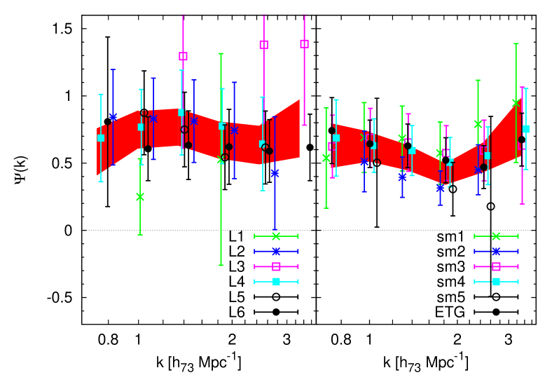
Refer to caption
Figure 12: Results of the ΨΨ\Psi-statistics which probes the third-order galaxy biasing parameters of our lens samples. Plotted is r1/(b3r2)subscript𝑟1subscript𝑏3subscript𝑟2r_{1}/(b_{3}r_{2}) as function of scale k=2/R=2/(fK(χmax)θ)𝑘2𝑅2subscript𝑓Ksubscript𝜒max𝜃k=\sqrt{2}/R=\sqrt{2}/(f_{\rm K}(\chi_{\rm max})\theta) for the angular range 1θ<10superscript1𝜃superscript101^{\prime}\leq\theta<10^{\prime}. Used are only significant measurements in the low-z𝑧z samples. Luminosity samples are in the left panel, stellar mass samples and the ETG sample in the right panel. Data points with uncertainties larger than σΨ>0.8subscript𝜎Ψ0.8\sigma_{\Psi}>0.8 are not shown. The shaded area indicates the mean and standard deviation of the mean of combined samples. L1-L6: Mrsubscript𝑀𝑟M_{r}-luminosities increasing from -17.8 mag to -22.4 mag; sm1-sm5: increasing stellar masses from 7×10⁹M7superscript109subscript𝑀direct-product7\times 10^{9}\,M_{\odot} to 1011Msuperscript1011subscript𝑀direct-product10^{11}\,M_{\odot}; ETG: early-type galaxies.

6 Discussion

We performed a G3L analysis of approximately 100 square degree of the CFHTLenS data set. The data is endowed with photometric redshifts of galaxies and lensfit estimates of the PSF-corrected source ellipticities. For the first time, the signal-to-noise of the lensing data is sufficient to measure third-order galaxy-galaxy lensing as a function of lens luminosity, stellar mass and galaxy type. The work of Simon et al. (2008), analysing the RCS1 data, demonstrated that G3L measurements are principally possible with contemporary lensing surveys. This is confirmed by this study. We further subdivided the lens samples in Mrsubscript𝑀𝑟M_{r}-luminosities, stellar masses, SED types, and a “low-z𝑧z” (0.2zphoto<0.440.2subscript𝑧photo0.440.2\leq z_{\rm photo}<0.44) and a “high-z𝑧z” (0.44zphoto<0.60.44subscript𝑧photo0.60.44\leq z_{\rm photo}<0.6) redshift bin by utilising the photometric redshifts of the lenses. We presented the G3L measurements in terms of aperture statistics that probes the angular bispectrum of the (projected) matter-galaxy three-point correlations. In one case (“lens-lens-shear”), the measurements quantify correlations between two lens positions and the surface matter density around the lens pair; this can be interpreted as excess surface mass density about galaxy pairs (Simon et al., 2012). In the other case (“lens-shear-shear”), it expresses correlations between a lens position and the surface mass density in two different directions close to the lens. The here adopted G3L aperture statistics has the practical advantage to separate E- and B/P-modes from these measurements, which is utilised to detect signatures of possible systematics in the data. On this level, no significant G3L systematics signals were detected.

To reduce the impact due to intrinsic alignments of sources, we separated lens and source galaxy samples physically from each other by exploiting the photometric redshifts in the survey. We showed that in the ideal case of no radial overlap, neither II-correlations nor GI-correlations contribute to the correlator. Owing to the uncertainty in the galaxy redshifts, however, perfectly non-overlapping distributions are hard to achieve. We found that our low-z𝑧z lens samples have still a small overlap of 4%similar-toabsentpercent4\sim 4\% with the source sample, the high-z𝑧z samples a moderate overlap of 12%similar-toabsentpercent12\sim 12\% (overlap of redshift probability distribution functions). Because of the small overlap, at least for the low-z𝑧z samples we do not expect significant contributions from intrinsic alignment correlations. To test the degree of contamination by GI- and II-correlations, we compared the aperture statistics of the combined sm3-sm5 samples, both low-z𝑧z (z¯d=0.35subscript¯𝑧d0.35\bar{z}_{\rm d}=0.35) and high-z𝑧z (z¯d=0.51subscript¯𝑧d0.51\bar{z}_{\rm d}=0.51), for two cases. In one case, we selected sources by 0.65zphoto<1.20.65subscript𝑧photo1.20.65\leq z_{\rm photo}<1.2 (z¯s=0.93subscript¯𝑧s0.93\bar{z}_{\rm s}=0.93) as before. In the second case, we were more conservative by selecting only sources within 0.8zphoto<1.20.8subscript𝑧photo1.20.8\leq z_{\rm photo}<1.2 (z¯s=1.02subscript¯𝑧s1.02\bar{z}_{\rm s}=1.02), thereby discarding about one third of our sources. However, the latter case reduced the overlap from 3.3%percent3.33.3\% (10.9%percent10.910.9\%) to 0.6%percent0.60.6\% (2.5%percent2.52.5\%) for the low-z𝑧z (high-z𝑧z) sample. The statistics were normalised by dχqggm(χ)differential-d𝜒subscript𝑞ggm𝜒\int{\rm d}\chi q_{\rm ggm}(\chi) (dχqmmg(χ)differential-d𝜒subscript𝑞mmg𝜒\int{\rm d}\chi q_{\rm mmg}(\chi)) to compensate the signal change owing to the different source depths. The maximum signal increase is 30%similar-toabsentpercent30\sim 30\% for 𝒩Map2delimited-⟨⟩𝒩superscriptsubscript𝑀ap2\langle{\cal N}M_{\rm ap}^{2}\rangle of the high-z𝑧z lens sample. Fig. 13 shows the difference in normalised statistics for fixed lens samples but varying source depths. Here we assumed that fK(χmax)subscript𝑓Ksubscript𝜒maxf_{\rm K}(\chi_{\rm max}) is identical for both compared signals, i.e., both signals were differenced at the same aperture scale radius. This assumption is accurate within a few percent here. As expected, the difference is consistent with zero, the level of GI/II-systematics in the statistics is therefore negligible within the measurement errors.
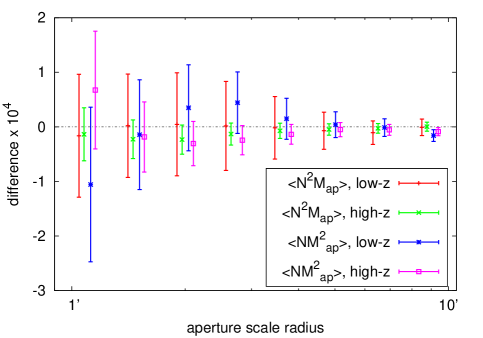
Refer to caption
Figure 13: Plotted are the differences of 𝒩2Map(θ)/dχqggm(χ)delimited-⟨⟩superscript𝒩2subscript𝑀ap𝜃differential-d𝜒subscript𝑞ggm𝜒\langle{\cal N}^{2}M_{\rm ap}\rangle(\theta)/\int{\rm d}\chi\,q_{\rm ggm}(\chi) for sources with zphoto0.65subscript𝑧photo0.65z_{\rm photo}\geq 0.65 and zphoto0.8subscript𝑧photo0.8z_{\rm photo}\geq 0.8, and the analogue for 𝒩Map2(θ)/dχqmmg(χ)delimited-⟨⟩𝒩subscriptsuperscript𝑀2ap𝜃differential-d𝜒subscript𝑞mmg𝜒\langle{\cal N}M^{2}_{\rm ap}\rangle(\theta)/\int{\rm d}\chi\,q_{\rm mmg}(\chi). For fixed lens samples (sm3-5 combined; either low-z𝑧z or high-z𝑧z), the result is expected to be consistent with zero. Note that neighbouring error bars are correlated.

As second possible source of systematics we identified the magnification of the lens number densities by matter fluctuations in front of the lenses. To first order this effect is comparable to the aperture mass skewness Map3(θ)delimited-⟨⟩superscriptsubscript𝑀ap3𝜃\langle M_{\rm ap}^{3}(\theta)\rangle associated with sources at redshift zs0.4similar-tosubscript𝑧s0.4z_{\rm s}\sim 0.4. We estimated this effect to be of the order of 108less-than-or-similar-toabsentsuperscript108\lesssim 10^{-8} at θ1similar-to𝜃1\theta\sim 1 arcmin. We therefore conclude in comparison with our measurements that in the range 1θ10less-than-or-similar-tosuperscript1𝜃less-than-or-similar-tosuperscript101^{\prime}\lesssim\theta\lesssim 10^{\prime} the lens number density magnification effect is negligible for both 𝒩2Mapdelimited-⟨⟩superscript𝒩2subscript𝑀ap\langle{\cal N}^{2}M_{\rm ap}\rangle and for 𝒩Map2delimited-⟨⟩𝒩subscriptsuperscript𝑀2ap\langle{\cal N}M^{2}_{\rm ap}\rangle. For a more detailed investigation of systematics, however, realistic models of intrinsic alignments and magnification for third-order correlations are required, which are currently unavailable.

The observed aperture statistics depend on the redshift distributions of lenses and sources. Results of the statistics would hence differ when changing the source or lens redshift distribution, even if the underlying comoving spatial 3D matter-galaxy bispectrum were unchanged throughout the light-cone. In order to partially correct for this effect, we employed a new technique that normalises the aperture statistics with the lensing efficiency and relates angular scales to effective spatial scales; this yields two kinds of galaxy-matter bispectra ggm(R)subscriptggm𝑅{\cal B}_{\rm ggm}(R) and mmg(R)subscriptmmg𝑅{\cal B}_{\rm mmg}(R), originating from 𝒩2Mapdelimited-⟨⟩superscript𝒩2subscript𝑀ap\langle{\cal N}^{2}M_{\rm ap}\rangle and 𝒩Map2delimited-⟨⟩𝒩superscriptsubscript𝑀ap2\langle{\cal N}M_{\rm ap}^{2}\rangle, respectively. The normalised statistics obtained are basically band bispectra due to the smoothing of the exponential u𝑢u-filter in k𝑘k-space and the radial smoothing of the lensing kernels. Only by means of our or similar normalisation schemes, measurements for different lens samples or same galaxy selections at different redshifts become comparable. In particular, the application of our normalisation simplifies the comparison with results from future studies. The problem of unnormalised measurements becomes particularly obvious for 𝒩2Mapdelimited-⟨⟩superscript𝒩2subscript𝑀ap\langle{\cal N}^{2}M_{\rm ap}\rangle of the low-z𝑧z L1 sample in Fig. 6 (top left panel) in comparison to the L6 sample in the same panel: for θ2greater-than-or-equivalent-to𝜃2\theta\gtrsim 2 arcmin both measurements are basically identical, although the normalisation reveals that the lower luminosity galaxies have a smaller bispectrum amplitude (Fig. 11, left panel). This effect results from a completely different redshift distribution of the L1 lenses that, due to sample incompleteness, have a mean redshift of z0.22similar-to𝑧0.22z\sim 0.22 instead of L6’s z0.34similar-to𝑧0.34z\sim 0.34.

We estimated the measurement errors directly from the data by Jackknifing the signal variance across the survey pointings. Ideally, with statistically independent pointings this would properly account for uncertainties due to source shape noise, sampling noise and cosmic variance. However, the pointings are bundled together in large fields W1-W4 with extensions of several degrees across the sky. This makes pointings of the same field partly correlated. Therefore, the cited uncertainties are probably somewhat too optimistic in the sense that they underestimate the cosmic variance.

To refine the previous RCS1 measurement in Simon et al. (2008) for different galaxy populations and to investigate the dependences of bispectra amplitudes on galaxy populations, we focussed here on equally-sized apertures. This gives most weight to the equilateral bispectra. We found that the aperture statistics are reasonably well described by a power law on angular scales ranging from roughly two arcmin to ten arcmin. On smaller angular scales, we observe evidence for a change of slope, but we are also increasingly affected by the transformation bias. For instance, 𝒩2Mapdelimited-⟨⟩superscript𝒩2subscript𝑀ap\langle{\cal N}^{2}M_{\rm ap}\rangle of the fainter low-z𝑧z L4 sample clearly flattens below 2similar-toabsent2\sim 2 arcmin. Qualitatively, this behaviour is also observed in the semi-analytic galaxy models studied in Saghiha et al. (2012), see their Fig. 8. A similar change of slope, maybe also a steepening, is visible for the 𝒩Map2delimited-⟨⟩𝒩subscriptsuperscript𝑀2ap\langle{\cal N}M^{2}_{\rm ap}\rangle statistics of the luminosity samples. A comparison of galaxy models to our measurements requires a careful replication of the galaxy sample selections, their uncertainties, and the survey incompleteness. Moreover, as concluded in Saghiha et al. (2012), no reliable galaxy model is currently available to predict the correct amplitude of G3L measurements – or to even double-check whether our results may be strongly effected by galaxy selection effects. We hence postpone this task to a future paper.

Table 4: Values of the normalised galaxy-matter bispectra ggm(R)subscriptggm𝑅{\cal B}_{\rm ggm}(R) (top half) and mmg(R)subscriptmmg𝑅{\cal B}_{\rm mmg}(R) (bottom half) at R=1h1001Mpc𝑅1superscriptsubscript1001MpcR=1\,h_{100}^{-1}\rm Mpc for the late-type (LTG) and early-type (ETG) galaxy sample.
Sample low-z𝑧z high-z𝑧z
ETG +1.040.17+0.17×10⁴superscriptsubscript1.040.170.17superscript104+1.04_{-0.17}^{+0.17}\times 10^{-4} +9.481.23+1.19×10⁵superscriptsubscript9.481.231.19superscript105+9.48_{-1.23}^{+1.19}\times 10^{-5}
LTG +4.375.01+9.21×10⁶superscriptsubscript4.375.019.21superscript106+4.37_{-5.01}^{+9.21}\times 10^{-6} +1.071.02+1.67×10⁵superscriptsubscript1.071.021.67superscript105+1.07_{-1.02}^{+1.67}\times 10^{-5}
ETG +5.981.41+1.35×10⁵superscriptsubscript5.981.411.35superscript105+5.98_{-1.41}^{+1.35}\times 10^{-5} +1.420.92+1.37×10⁵superscriptsubscript1.420.921.37superscript105+1.42_{-0.92}^{+1.37}\times 10^{-5}
LTG +6.934.46+9.91×10⁶superscriptsubscript6.934.469.91superscript106+6.93_{-4.46}^{+9.91}\times 10^{-6} 1.391.62+0.95×10⁵superscriptsubscript1.391.620.95superscript105-1.39_{-1.62}^{+0.95}\times 10^{-5}

The measurements of ggmsubscriptggm{\cal B}_{\rm ggm} utilising ETG and LTG pairs (subdivision of the combined L5/L6 sample) show that the excess mass around pairs is a strong function of galaxy type. The high excess mass signal of ETG is comparable to the strong signal of pairs in our sm-samples with stellar masses of 1011Msimilar-toabsentsuperscript1011subscript𝑀direct-product\sim 10^{11}\,M_{\odot}, whereas the excess mass of LTG is consistent with zero in our case (Table 4). A plausible explanation for this is the fact that many early-type galaxies in the ETG sample (M6×1010Mdelimited-⟨⟩subscript𝑀6superscript1010subscript𝑀direct-product\langle M_{\ast}\rangle\approx 6\times 10^{10}\,M_{\odot}) are satellites in dense cluster environments, whereas LTG are frequently field galaxies. This was, for instance, found by the GGL study of Mandelbaum et al. (2006) in SDSS. The splitting into ETG from over-dense and under-dense regions that was conducted in this study is actually comparable to the lens-lens-shear correlation function because the G3L correlator gives more weight to pairs in cluster environments, simply because more pairs are found in these regions. Recently, Saghiha et al. (2012) studied the excess mass for two state-of-the-art semi-analytic galaxy models. Although the G3L amplitudes and colour distributions of the two considered models are inconsistent, both models predict a large difference in 𝒩2Mapdelimited-⟨⟩superscript𝒩2subscript𝑀ap\langle{\cal N}^{2}M_{\rm ap}\rangle for zd=0.17subscript𝑧d0.17z_{\rm d}=0.17 red and blue galaxies up to a factor of 102similar-toabsentsuperscript102\sim 10^{2} at θ2arcminsimilar-to𝜃2arcmin\theta\sim 2\,\rm arcmin. With our uncertainties in the LTG signal, we estimate the difference to be at least a factor 10similar-toabsent10\sim 10, strongly confirming the previous prediction.

By forming ratios of normalised bispectra, our new statistic Ψ(R):=mmg(R)/ggm(R)assignΨ𝑅subscriptmmg𝑅subscriptggm𝑅\Psi(R):={\cal B}_{\rm mmg}(R)/{\cal B}_{\rm ggm}(R) approximately yields the ratio r1/(r2b3)subscript𝑟1subscript𝑟2subscript𝑏3r_{1}/(r_{2}b_{3}) of (smoothed) third-order biasing parameters (SW05). The details of the smoothing are determined by the shapes of the u𝑢u-filter, the peaked kernels qmmg,qggmsubscript𝑞mmgsubscript𝑞ggmq_{\rm mmg},q_{\rm ggm}, and to some extent also the matter bispectrum (Appendix D). Deviations of ΨΨ\Psi from unity indicate galaxies that not faithfully trace the underlying matter density field, i.e., biased galaxies. This new technique for investigating galaxy bias with lensing advances the methodology of van Waerbeke (1998) and Schneider (1998) that focus on second-order galaxy bias. The application of the latter found that galaxies are generally biased tracers (Hoekstra et al., 2001; Simon et al., 2007; Jullo et al., 2012). We confirm this finding by employing third-order galaxy-matter correlations.

7 Conclusions

  • We detect G3L with unprecedented high significance in the CFHTLenS for galaxy populations of different luminosity, stellar mass, and SED type. This applies to both third-order galaxy-galaxy-matter correlations (ggmsubscriptggm{\cal B}_{\rm ggm}) and galaxy-matter-matter correlations (mmgsubscriptmmg{\cal B}_{\rm mmg}).

  • We find that the (equilateral) galaxy-matter bispectra are, within the remaining statistical errors, reasonably well scale-invariant for the spatial (comoving) scales 0.3Mpc1k2.2Mpc1less-than-or-similar-to0.3superscriptMpc1𝑘less-than-or-similar-to2.2superscriptMpc10.3\,{\rm Mpc}^{-1}\lesssim k\lesssim 2.2\,{\rm Mpc}^{-1}. On smaller scales, not included in our power-law fits, there are indications of deviations from the power-law shape in several cases.

  • The low-z𝑧z and high-z𝑧z counterparts of the same lens samples yield very similar bispectra amplitudes ggmsubscriptggm{\cal B}_{\rm ggm} (Fig. 11) and slopes (Fig. 9). This points to little evolution of the bispectrum between redshift z0.30.5similar-to𝑧0.30.5z\sim 0.3-0.5, especially for our Mrsubscript𝑀𝑟M_{r}-selected galaxies. There is, however, some evidence for a change in the amplitude of ggmsubscriptggm{\cal B}_{\rm ggm} for stellar-mass selected galaxies below 1011Msimilar-toabsentsuperscript1011subscriptMdirect-product\sim 10^{11}\,{\rm M}_{\odot}: high-z𝑧z lenses show a lower amplitude than the low-z𝑧z lenses (right panel of Fig. 11). This implies an increase of excess mass about pairs of galaxies of fixed stellar mass with time, as, e.g., may be expected in a CDM scenario due to the continuous accretion of matter. Evolution trends of mmgsubscriptmmg{\cal B}_{\rm mmg} are unclear due to the measurement uncertainties in the high-z𝑧z samples.

  • For ggmsubscriptggm{\cal B}_{\rm ggm} the slope and the amplitude is a changing function of galaxy luminosity, stellar mass and galaxy type. The amplitude change is also observed for mmgsubscriptmmg{\cal B}_{\rm mmg}. Brighter or more massive galaxies (by stellar mass) exhibit a steeper bispectrum, which implies that the excess mass is more concentrated in these cases. Moreover, there is a clear trend towards higher amplitudes for both more luminous and more massive galaxies. This shows that more luminous or massive galaxies, or galaxy pairs in the case of ggmsubscriptggm{\cal B}_{\rm ggm}, inhibit denser environments than fainter or lighter galaxies.

  • We observe a strong signal for the excess mass around early-type galaxies (ETG) pairs. Late-type galaxy pairs (LTG), on the other hand, have a signal that is consistent with zero when studied as aperture statistics. This remarkable observation is in excellent agreement with the recent prediction of Saghiha et al. (2012) based on semi-analytic galaxy models. The measurement therefore suggests that virtually all signal in this magnitude range originates from ETG pairs, and possibly mixed pairs of ETG and LTG, rather than from LTG pairs. This can be explained by the fact that a large fraction of ETG are satellite galaxies in cluster. By explicitly mapping out the excess mass around LTG and ETG galaxy pairs we have also found that both maps are fundamentally different in their amplitudes as well as in their general appearance.

  • The mismatch between ggmsubscriptggm{\cal B}_{\rm ggm} and mmgsubscriptmmg{\cal B}_{\rm mmg} for the same lens galaxy sample immediately indicates galaxies biased with respect to the matter distribution. This mismatch is captured by the galaxy bias statistics Ψ(R)Ψ𝑅\Psi(R) (Fig. 12) that shows for our low-z𝑧z samples values comparable for a wide range of galaxy luminosities and stellar masses. Therein, we probe the non-linear regime on scales smaller than k0.8Mpc1similar-to𝑘0.8superscriptMpc1k\sim 0.8\,\rm Mpc^{-1}. We find best constraints on Ψ(R)Ψ𝑅\Psi(R) with the stellar mass samples, which has for all samples sm1-sm5 and scales combined (minimum-variance weighted) an average value of Ψ¯=0.51±0.07¯Ψplus-or-minus0.510.07\overline{\Psi}=0.51\pm 0.07. This shows – for the first time employing third-order lensing statistics – that galaxies are biased tracer of the matter density field. Although Ψ(R)Ψ𝑅\Psi(R) indicates that the ratio r1/(r2b3)subscript𝑟1subscript𝑟2subscript𝑏3r_{1}/(r_{2}b_{3}) stays relatively constant with scale, with a possible shallow local minimum at k1.8Mpc1𝑘1.8superscriptMpc1k\approx 1.8\,\rm Mpc^{-1}, the additionally observed change of the bispectrum amplitudes with galaxy luminosity or mass means that the individual bias parameters have to differ between the galaxy samples.

  • Finally, we emphasise that theory is lacking behind in interpreting the G3L measurements. Reliable model predictions , e.g., in the vein of Takada & Jain (2003), are needed, not only to properly interpret the measurements, but also to gain a better understanding of systematics and to verify that selection effects in the data do not spoil the measurement.

Acknowledgements

We thank Stefan Hilbert for useful discussions and Hananeh Saghiha for verifying our correlator code output with hers on simulated data.

This work is based on observations obtained with MegaPrime/MegaCam, a joint project of CFHT and CEA/IRFU, at the Canada-France-Hawaii Telescope (CFHT) which is operated by the National Research Council (NRC) of Canada, the Institut National des Sciences de l’Univers of the Centre National de la Recherche Scientifique (CNRS) of France, and the University of Hawaii. This research used the facilities of the Canadian Astronomy Data Centre operated by the National Research Council of Canada with the support of the Canadian Space Agency. We thank the CFHT staff for successfully conducting the CFHTLS observations and in particular Jean-Charles Cuillandre and Eugene Magnier for the continuous improvement of the instrument calibration and the Elixir detrended data that we used. We also thank TERAPIX for the quality assessment and validation of individual exposures during the CFHTLS data acquisition period, and Emmanuel Bertin for developing some of the software used in this study. CFHTLenS data processing was made possible thanks to significant computing support from the NSERC Research Tools and Instruments grant program, and to HPC specialist Ovidiu Toader. The early stages of the CFHTLenS project were made possible thanks to the support of the European Commission’s Marie Curie Research Training Network DUEL (MRTN-CT-2006-036133) which directly supported members of the CFHTLenS team (C. Bonnett, L. Fu, H. Hoekstra, B.T.P. Rowe, P. Simon, M. Velander) between 2007 and 2011 in addition to providing travel support and expenses for team meetings.

T. Erben is supported by the Deutsche Forschungsgemeinschaft through project ER 327/3-1 and, with P. Simon and P. Schneider, by the Transregional Collaborative Research Centre TR33 - ”The Dark Universe”. C. Heymans, H. Hoekstra & B.T.P. Rowe acknowledge support from the European Research Council under the EC FP7 grant numbers 240185 (CH), 279396 (H. Hoekstra+ES) & 240672 (BR). L. van Waerbeke acknowledges support from the Natural Sciences and Engineering Research Council of Canada (NSERC) and the Canadian Institute for Advanced Research (CIfAR, Cosmology and Gravity program). H. Hildebrandt is supported by the Marie Curie IOF 252760, a CITA National Fellowship, and the DFG grant Hi 1495/2-1. H. Hoekstra and E. Semboloni also acknowledge support from Marie Curie IRG grant 230924 and the Netherlands Organisation for Scientific Research grant number 639.042.814. T.D. Kitching acknowledges support from a Royal Society University Research Fellowship. Y. Mellier acknowledges support from CNRS/INSU (Institut National des Sciences de l’Univers) and the Programme National Galaxies et Cosmologie (PNCG). L. Fu acknowledges support from NSFC grants 11103012 and 10878003, Innovation Program 12ZZ134 and Chen Guang project 10CG46 of SMEC, and STCSM grant 11290706600 & Pujiang Program 12PJ1406700. M.J. Hudson acknowledges support from the Natural Sciences and Engineering Research Council of Canada (NSERC). T. Schrabback acknowledges support from NSF through grant AST-0444059-001, SAO through grant GO0-11147A, and NWO. M. Velander acknowledges support from the Netherlands Organization for Scientific Research (NWO) and from the Beecroft Institute for Particle Astrophysics and Cosmology. C. Bonnett is supported by the Spanish Science Ministry AYA2009-13936 Consolider-Ingenio CSD2007-00060, project 2009SGR1398 from Generalitat de Catalunya and by the European Commission’s Marie Curie Initial Training Network CosmoComp (PITN-GA-2009-238356).

Author Contributions: All authors contributed to the development and writing of this paper. The authorship list reflects the lead authors of this paper (P. Simon, T. Erben, and P. Schneider) followed by two alphabetical groups. The first alphabetical group includes key contributers to the science analysis and interpretation in this paper, the founding core team and those whose long-term significant effort produced the final CFHTLenS data product. The second group covers members of the CFHTLenS team who made a significant contribution to either the project, this paper or both. C. Heymans and L. van Waerbeke co-led the CFHTLenS collaboration.

References

  • Bartelmann & Schneider (2001) Bartelmann M., Schneider P., 2001, Phys. Rep., 340, 291
  • Benitez (2000) Benitez N., 2000, ApJ, 536, 571
  • Benjamin et al. (2012) Benjamin J., van Waerbeke L., Heymans C., et al. 2012, MNRAS, submitted, arXiv:1212.3327
  • Bernardeau et al. (2003) Bernardeau F., van Waerbeke L., Mellier Y., 2003, A&A, 397, 405
  • Brainerd et al. (1996) Brainerd T., Blandford R. D., Smail I., 1996, ApJ, 466, 623
  • Chabrier (2003) Chabrier G., 2003, Publ. Astron. Soc. Pacific, 115, 763
  • Cooray & Sheth (2002) Cooray A., Sheth R., 2002, Phys. Rev., 372, 1
  • Crittenden et al. (2002) Crittenden R. G., Natarajan P., Pen U.-L., Theuns T., 2002, ApJ, 568, 20
  • Dodelson (2003) Dodelson S., 2003, Modern cosmology. Academic Press, Amsterdam (Netherlands)
  • Erben et al. (2009) Erben T., Hildebrandt H., Lerchster M., Hudelot P., Benjamin J., van Waerbeke L., Schrabback T., Brimioulle F., Cordes O., Dietrich J. P., Holhjem K., Schirmer M., Schneider P., 2009, A&A, 493, 1197
  • Erben et al. (2012) Erben T., Hildebrandt H., Miller L., et al. 2012, MNRAS, submitted, arXiv:1210.8156
  • Fischer et al. (1999) Fischer P., McKay T., Sheldon E., et al., 1999, arXiv:9912119
  • Gladders & Yee (2005) Gladders M. D., Yee H. K. C., 2005, ApJ Suppl., 157, 1
  • Goldberg & Bacon (2005) Goldberg D. M., Bacon D. J., 2005, ApJ, 619, 741
  • Goldberg & Natarajan (2002) Goldberg D. M., Natarajan P., 2002, ApJ, 564, 65
  • Groth & Peebles (1977) Groth E. J., Peebles P. J. E., 1977, ApJ, 217, 385
  • Hartlap et al. (2007) Hartlap J., Simon P., Schneider P., 2007, A&A, 464, 399
  • Hetterscheidt et al. (2007) Hetterscheidt M., Simon P., Schirmer M., Hildebrandt H., Schrabback T., Erben T., Schneider P., 2007, A&A, 468, 859
  • Heymans et al. (2012) Heymans C., Grocutt E., Heavens A., et al. 2012, in preparation
  • Heymans et al. (2012) Heymans C., Van Waerbeke L., Miller L., et al. 2012, accepted by MNRAS, arXiv:1210.0032
  • Heymans et al. (2006) Heymans C., White M., Heavens A., Vale C., van Waerbeke L., 2006, MNRAS, 371, 750
  • Hildebrandt et al. (2012) Hildebrandt H., Erben T., Kuijken K., et al. 2012, MNRAS, 421, 2355
  • Hildebrandt et al. (2009) Hildebrandt H., van Waerbeke L., Erben T., 2009, A&A, 507, 683
  • Hinkley (1969) Hinkley D. V., 1969, Biometrika, 56, 635
  • Hirata & Seljak (2004) Hirata C. M., Seljak U., 2004, Phys. Rev. D, 70, 063526
  • Hoekstra et al. (2003) Hoekstra H., Franx M., Kuijken K., Carlberg R. G., Yee H. K. C., 2003, MNRAS, 340, 609
  • Hoekstra & Jain (2008) Hoekstra H., Jain B., 2008, Annual Review of Nuclear and Particle Science, 58, 99
  • Hoekstra et al. (2002) Hoekstra H., Van Waerbeke L., Gladders M. D., 2002, ApJ, 577, 604
  • Hoekstra et al. (2001) Hoekstra H., Yee H. K. C., Gladders M. D., 2001, ApJ(Lett), 558, L11
  • Hoekstra et al. (2004) Hoekstra H., Yee H. K. C., Gladders M. D., 2004, ApJ, 606, 67
  • Hudson et al. (1998) Hudson M. J., Gwyn S. D. J., Dahle H., Kaiser N., 1998, ApJ, 503, 531
  • Jarvis et al. (2004) Jarvis M., Bernstein G., Jain B., 2004, MNRAS, 352, 338
  • Joachimi et al. (2011) Joachimi B., Mandelbaum R., Abdalla F. B., Bridle S. L., 2011, A&A, 527, A26
  • Jullo et al. (2012) Jullo E., Rhodes J., Kiessling A., Taylor J. E., Massey R., Berge J., Schimd C., Kneib J.-P., Scoville N., 2012, ApJ, 750, 37
  • Kaiser (1992) Kaiser N., 1992, ApJ, 388, 272
  • Kaiser & Squires (1993) Kaiser N., Squires G., 1993, ApJ, 404, 441
  • Kilbinger et al. (2012) Kilbinger M., Fu L., Heymans C., et al. 2012, MNRAS, submitted, arXiv:1212.3338
  • Kilbinger et al. (2006) Kilbinger M., Schneider P., Eifler T., 2006, A&A, 457, 15
  • Kitching et al. (2008) Kitching T. D., Miller L., Heymans C. E., van Waerbeke L., Heavens A. F., 2008, MNRAS, 390, 149
  • Kleinheinrich et al. (2006) Kleinheinrich M., Schneider P., Rix H.-W., Erben T., Wolf C., Schirmer M., Meisenheimer K., Borch A., Dye S., Kovacs Z., Wisotzki L., 2006, A&A, 455, 441
  • Komatsu et al. (2011) Komatsu E., Smith K. M., Dunkley J., et al. 2011, ApJ Suppl., 192, 18
  • Landy & Szalay (1993) Landy S. D., Szalay A. S., 1993, ApJ, 412, 64
  • Leauthaud et al. (2012) Leauthaud A., Tinker J., Bundy K., et al. 2012, ApJ, 744, 159
  • Mandelbaum et al. (2006) Mandelbaum R., Hirata C. M., Broderick T., Seljak U., Brinkmann J., 2006, MNRAS, 370, 1008
  • Mandelbaum et al. (2006) Mandelbaum R., Seljak U., Kauffmann G., Hirata C. M., Brinkmann J., 2006, MNRAS, 368, 715
  • Mandelbaum et al. (2012) Mandelbaum R., Slosar A., Baldauf T., Seljak U., Hirata C. M., Nakajima R., Reyes R., Smith R. E., 2012, ArXiv e-prints
  • McKay et al. (2001) McKay T. A., Sheldon E. S., Racusin J., et al. 2001, arXiv:0108013
  • Meylan et al. (2006) Meylan G., Jetzer P., North P., Schneider P., Kochanek C. S., Wambsganss J., 2006, in G. Meylan, P. Jetzer, P. North, P. Schneider, C. S. Kochanek, & J. Wambsganss ed., Saas-Fee Advanced Course 33: Gravitational Lensing: Strong, Weak and Micro
  • Miller et al. (2012) Miller L., Heymans C., Kitching T. D., et al. 2012, MNRAS, submitted, arXiv:1210.8201
  • Miller et al. (2007) Miller L., Kitching T. D., Heymans C., Heavens A. F., van Waerbeke L., 2007, MNRAS, 382, 315
  • Narayan (1989) Narayan R., 1989, ApJ(Lett), 339, L53
  • Navarro et al. (1996) Navarro J. F., Frenk C. S., White S. D. M., 1996, ApJ, 462, 563
  • Norberg et al. (2009) Norberg P., Baugh C. M., Gaztañaga E., Croton D. J., 2009, MNRAS, 396, 19
  • Parker et al. (2007) Parker L. C., Hoekstra H., Hudson M. J., van Waerbeke L., Mellier Y., 2007, ApJ, 669, 21
  • Peacock (1999) Peacock J. A., 1999, Cosmological physics. Cambridge University Press
  • Peebles (1980) Peebles P. J. E., 1980, The large-scale structure of the universe. Princeton University Press, USA
  • Pen et al. (2003) Pen U.-L., Lu T., van Waerbeke L., Mellier Y., 2003, MNRAS, 346, 994
  • Pen et al. (2003) Pen U.-L., Zhang T., van Waerbeke L., Mellier Y., Zhang P., Dubinski J., 2003, ApJ, 592, 664
  • Reyes et al. (2010) Reyes R., Mandelbaum R., Seljak U., et al. 2010, Nat, 464, 256
  • Saghiha et al. (2012) Saghiha H., Hilbert S., Schneider P., Simon P., 2012, A&A, 547, A77
  • Schneider (1998) Schneider P., 1998, ApJ, 498, 43
  • Schneider (2003) Schneider P., 2003, A&A, 408, 829
  • Schneider (2006) Schneider P., 2006, in G. Meylan, P. Jetzer, P. North, P. Schneider, C. S. Kochanek, & J. Wambsganss ed., Saas-Fee Advanced Course 33: Gravitational Lensing: Strong, Weak and Micro Part 3: Weak gravitational lensing. pp 269–451
  • Schneider et al. (2005) Schneider P., Kilbinger M., Lombardi M., 2005, A&A, 431, 9
  • Schneider et al. (1998) Schneider P., Van Waerbeke L., Jain B., Kruse G., 1998, MNRAS, 296, 873
  • Schneider et al. (2002) Schneider P., van Waerbeke L., Mellier Y., 2002, A&A, 389, 729
  • Schrabback & CFHTLenS team (2012) Schrabback T., CFHTLenS team 2012, in preparation
  • Seljak et al. (2005) Seljak U., Makarov A., Mandelbaum R., Hirata C. M., Padmanabhan N., McDonald P., Blanton M. R., Tegmark M., Bahcall N. A., Brinkmann J., 2005, Phys. Rev. D, 71, 043511
  • Seljak & Warren (2004) Seljak U., Warren M. S., 2004, MNRAS, 355, 129
  • Semboloni et al. (2011) Semboloni E., Schrabback T., van Waerbeke L., Vafaei S., Hartlap J., Hilbert S., 2011, MNRAS, 410, 143
  • Shao (1986) Shao J., 1986, Ann. Stat., 14, 1322
  • Sheldon et al. (2004) Sheldon E. S., Johnston D. E., Frieman J. A., Scranton R., McKay T. A., Connolly A. J., Budavári T., Zehavi I., Bahcall N. A., Brinkmann J., Fukugita M., 2004, AJ, 127, 2544
  • Simon et al. (2007) Simon P., Hetterscheidt M., Schirmer M., Erben T., Schneider P., Wolf C., Meisenheimer K., 2007, A&A, 461, 861
  • Simon et al. (2012) Simon P., Schneider P., Kübler D., 2012, A&A, in press, arXiv:1202.1927
  • Simon et al. (2008) Simon P., Watts P., Schneider P., Hoekstra H., Gladders M. D., Yee H. K. C., Hsieh B. C., Lin H., 2008, A&A, 479, 655
  • Springel et al. (2005) Springel V., White S. D. M., Jenkins A., et al. 2005, Nat, 435, 629
  • [SW05] Schneider & Watts (2005) [SW05] Schneider P., Watts P., 2005, A&A, 432, 783
  • Takada & Jain (2003) Takada M., Jain B., 2003, MNRAS, 340, 580
  • Tegmark & Bromley (1999) Tegmark M., Bromley B. C., 1999, ApJ(Lett), 518, L69
  • van Uitert et al. (2012) van Uitert E., Hoekstra H., Schrabback T., Gilbank D. G., Gladders M. D., Yee H. K. C., 2012, A&A, submitted, arXiv:1206.4304
  • van Uitert et al. (2011) van Uitert E., Hoekstra H., Velander M., Gilbank D. G., Gladders M. D., Yee H. K. C., 2011, A&A, submitted, arXiv:1107.4093
  • van Waerbeke (1998) van Waerbeke L., 1998, A&A, 334, 1
  • van Waerbeke (2010) van Waerbeke L., 2010, MNRAS, 401, 2093
  • Velander et al. (2011) Velander M., Kuijken K., Schrabback T., 2011, MNRAS, 412, 2665
  • Velander et al. (2012) Velander M., van Uitert E., Hoekstra H., et al. 2012, MNRAS, submitted
  • York et al. (2000) York D. G., Adelman J., Anderson J., et al. 2000, AJ, 120, 1579

Appendix A Multiplicative shear bias

Miller et al. (2012) discusses a calibration scheme for correlation function estimators involving shear estimates from the lensfit pipeline. For details, we refer the reader to the mentioned article, Sect. 8.3 and 8.4. Analogous to the calibration scheme of the two-point shear-shear correlation function detailed therein, we divide 𝒢~estsuperscript~𝒢est\tilde{\cal G}^{\rm est}, Eq. (2.3), and G~±estsuperscriptsubscript~𝐺plus-or-minusest\tilde{G}_{\pm}^{\rm est}, Eq. (2.3), by 1+K𝒢(ϑ1,ϑ2,ϕ3)1subscript𝐾𝒢subscriptitalic-ϑ1subscriptitalic-ϑ2subscriptitalic-ϕ31+K_{\cal G}(\vartheta_{1},\vartheta_{2},\phi_{3}) and 1+KG±(ϑ1,ϑ2,ϕ3)1subscript𝐾subscript𝐺plus-or-minussubscriptitalic-ϑ1subscriptitalic-ϑ2subscriptitalic-ϕ31+K_{G_{\pm}}(\vartheta_{1},\vartheta_{2},\phi_{3}), respectively. Both calibration factors are given by

1+K𝒢(ϑ1,ϑ2,ϕ3)1subscript𝐾𝒢subscriptitalic-ϑ1subscriptitalic-ϑ2subscriptitalic-ϕ3\displaystyle 1+K_{\cal G}(\vartheta_{1},\vartheta_{2},\phi_{3})
=i=1Ndj=1Ndk=1Nswk(1+mk)Δijkϑ1ϑ2ϕ3i=1Ndj=1Ndk=1NswkΔijkϑ1ϑ2ϕ3,absentsuperscriptsubscript𝑖1subscript𝑁dsuperscriptsubscript𝑗1subscript𝑁dsuperscriptsubscript𝑘1subscript𝑁ssubscript𝑤𝑘1subscript𝑚𝑘superscriptsubscriptΔ𝑖𝑗𝑘subscriptitalic-ϑ1subscriptitalic-ϑ2subscriptitalic-ϕ3superscriptsubscript𝑖1subscript𝑁dsuperscriptsubscript𝑗1subscript𝑁dsuperscriptsubscript𝑘1subscript𝑁ssubscript𝑤𝑘superscriptsubscriptΔ𝑖𝑗𝑘subscriptitalic-ϑ1subscriptitalic-ϑ2subscriptitalic-ϕ3\displaystyle=\frac{\sum\limits_{i=1}^{N_{\rm d}}\sum\limits_{j=1}^{N_{\rm d}}\sum\limits_{k=1}^{N_{\rm s}}w_{k}(1+m_{k})\Delta_{ijk}^{\vartheta_{1}\vartheta_{2}\phi_{3}}}{\sum\limits_{i=1}^{N_{\rm d}}\sum\limits_{j=1}^{N_{\rm d}}\sum\limits_{k=1}^{N_{\rm s}}w_{k}\Delta_{ijk}^{\vartheta_{1}\vartheta_{2}\phi_{3}}}\;,
1+KG±(ϑ1,ϑ2,ϕ3)1subscript𝐾subscript𝐺plus-or-minussubscriptitalic-ϑ1subscriptitalic-ϑ2subscriptitalic-ϕ3\displaystyle 1+K_{G_{\pm}}(\vartheta_{1},\vartheta_{2},\phi_{3})
=i=1Ndj=1Nsk=1Nswjwk(1+mj)(1+mk)Δijkϑ1ϑ2ϕ3i=1Ndj=1Nsk=1NswjwkΔijkϑ1ϑ2ϕ3.absentsuperscriptsubscript𝑖1subscript𝑁dsuperscriptsubscript𝑗1subscript𝑁ssuperscriptsubscript𝑘1subscript𝑁ssubscript𝑤𝑗subscript𝑤𝑘1subscript𝑚𝑗1subscript𝑚𝑘superscriptsubscriptΔ𝑖𝑗𝑘subscriptitalic-ϑ1subscriptitalic-ϑ2subscriptitalic-ϕ3superscriptsubscript𝑖1subscript𝑁dsuperscriptsubscript𝑗1subscript𝑁ssuperscriptsubscript𝑘1subscript𝑁ssubscript𝑤𝑗subscript𝑤𝑘superscriptsubscriptΔ𝑖𝑗𝑘subscriptitalic-ϑ1subscriptitalic-ϑ2subscriptitalic-ϕ3\displaystyle=\frac{\sum\limits_{i=1}^{N_{\rm d}}\sum\limits_{j=1}^{N_{\rm s}}\sum\limits_{k=1}^{N_{\rm s}}w_{j}w_{k}(1+m_{j})(1+m_{k})\Delta_{ijk}^{\vartheta_{1}\vartheta_{2}\phi_{3}}}{\sum\limits_{i=1}^{N_{\rm d}}\sum\limits_{j=1}^{N_{\rm s}}\sum\limits_{k=1}^{N_{\rm s}}w_{j}w_{k}\Delta_{ijk}^{\vartheta_{1}\vartheta_{2}\phi_{3}}}\;.

The multiplicative bias factors misubscript𝑚𝑖m_{i}, provided in the CFHTLenS catalogue333Publicly available under http://www.cadc-ccda.hia-iha.nrc-cnrc.gc.ca/community/CFHTLens/query.html for each source, are functions of the source signal-to-noise and angular size. Note that for non-vanishing values of 1+mi>01subscript𝑚𝑖01+m_{i}>0, the calibration is mathematically equivalent to employing the transformation ϵiϵi/(1+mi)maps-tosubscriptitalic-ϵ𝑖subscriptitalic-ϵ𝑖1subscript𝑚𝑖\epsilon_{i}\mapsto\epsilon_{i}/(1+m_{i}) and wiwi(1+mi)maps-tosubscript𝑤𝑖subscript𝑤𝑖1subscript𝑚𝑖w_{i}\mapsto w_{i}(1+m_{i}) in the estimators 𝒢~estsuperscript~𝒢est\widetilde{\cal G}^{\rm est} and G~±estsubscriptsuperscript~𝐺estplus-or-minus\widetilde{G}^{\rm est}_{\pm}.

Appendix B Lens samples supplement

B.1 Angular clustering of lenses

The angular correlation function ω(θ)𝜔𝜃\omega(\theta) of the lenses as a function of separation θ𝜃\theta is approximated by a simple power law (Peebles, 1980):

ω(θ)=Aω(θ1)λ+IC,𝜔𝜃subscript𝐴𝜔superscript𝜃superscript1𝜆IC\omega(\theta)=A_{\omega}\,\left(\frac{\theta}{1^{\prime}}\right)^{-\lambda}+{\rm IC}\;, (47)

where Aωsubscript𝐴𝜔A_{\omega} is the clustering strength at a separation of one arcmin, λ𝜆\lambda the slope of the correlation function and the constant offset IC, the integral constraint (Groth & Peebles, 1977). We find this fitting function to be a good description of ω(θ)𝜔𝜃\omega(\theta) between 0.2θ10less-than-or-similar-tosuperscript0.2𝜃less-than-or-similar-tosuperscript100^{\prime}\!\!.2\lesssim\theta\lesssim 10^{\prime}. The estimator of ω(θ)𝜔𝜃\omega(\theta) by Landy & Szalay (1993), employed for this paper, requires the repeated counting of galaxy pairs in separation bins for random realisations of unclustered galaxy distributions, factoring in the incompleteness of the survey. The figures quoted in Table 1 consider the masks of individual survey pointings, but presuming the same survey completeness within regions that are not masked out. For the final ω(θ)𝜔𝜃\omega(\theta), all pair counts from all individual survey fields are added so that, in effect, fields with more galaxies attain a higher weight in the average. The binned ω(θ)𝜔𝜃\omega(\theta) is stored as data vector 𝒅¯¯𝒅\overline{{\mn@boldsymbol{d}}}.

Pointing-to-pointing Jackknife sampling To estimate the statistical uncertainty of 𝒅¯¯𝒅\overline{{\mn@boldsymbol{d}}}, we prepare a set of Npsubscript𝑁pN_{\rm p} Jackknife samples 𝒅¯ijnsubscriptsuperscript¯𝒅jn𝑖\bar{{\mn@boldsymbol{d}}}^{\rm jn}_{i}, where 𝒅¯isubscript¯𝒅𝑖\bar{{\mn@boldsymbol{d}}}_{i} is the combined data vector omitting the i𝑖ith patch. The Jackknife covariance of the sample mean is then (Shao, 1986; Norberg et al., 2009):

C=1Npi=1NpΔ𝒅¯ijn[Δ𝒅¯ijn]t,C1subscript𝑁psuperscriptsubscript𝑖1subscript𝑁pΔsuperscriptsubscript¯𝒅𝑖jnsuperscriptdelimited-[]Δsuperscriptsubscript¯𝒅𝑖jnt\textbf{{C}}=\frac{1}{N_{\rm p}}\sum_{i=1}^{N_{\rm p}}\Delta\bar{{\mn@boldsymbol{d}}}_{i}^{\rm jn}\left[\Delta\bar{{\mn@boldsymbol{d}}}_{i}^{\rm jn}\right]^{\rm t}\;, (48)

where

Δ𝒅¯ijn:=(Np1)(𝒅¯𝒅¯ijn).assignΔsuperscriptsubscript¯𝒅𝑖jnsubscript𝑁p1¯𝒅superscriptsubscript¯𝒅𝑖jn\Delta\bar{{\mn@boldsymbol{d}}}_{i}^{\rm jn}:=(N_{\rm p}-1)(\bar{{\mn@boldsymbol{d}}}-\bar{{\mn@boldsymbol{d}}}_{i}^{\rm jn})\;. (49)

For Table 1, a power law fit is applied to the ensemble average 𝒅¯¯𝒅\overline{{\mn@boldsymbol{d}}} of all pointings, taking into account the Jackknife covariance C. The θ𝜃\theta-binning in 𝒅¯¯𝒅\overline{{\mn@boldsymbol{d}}} is also applied to the power law model, Eq. (47), by averaging the model over the width of each bin. Note that the inverse of C, required for the likelihood analysis of the model fit parameters, has to be corrected to obtain an unbiased estimator of the inverse covariance (Hartlap et al., 2007). Similar corrections of inverse covariances are applied throughout the paper without further mentioning.

B.2 Completeness of lens sample

Here we define a parameter that quantifies the completeness of our lens samples. First we define the comoving volume V(z1,z2)𝑉subscript𝑧1subscript𝑧2V(z_{1},z_{2}) confined by the redshift boundaries z1z<z2subscript𝑧1𝑧subscript𝑧2z_{1}\leq z<z_{2},

V(z1,z2)=Ωχ(z0)χ(z1)dχfK2(χ),𝑉subscript𝑧1subscript𝑧2Ωsuperscriptsubscript𝜒subscript𝑧0𝜒subscript𝑧1differential-d𝜒superscriptsubscript𝑓K2𝜒V(z_{1},z_{2})=\Omega\int_{\chi(z_{0})}^{\chi(z_{1})}{\rm d}\chi\,f_{\rm K}^{2}(\chi)\;, (50)

where ΩΩ\Omega is the solid angle of the patch field-of-view minus the solid angle of mask regions, and

χ(z)=DH0zdzE(z),𝜒𝑧subscript𝐷Hsuperscriptsubscript0𝑧dsuperscript𝑧𝐸superscript𝑧\chi(z)=D_{\rm H}\int_{0}^{z}\frac{{\rm d}z^{\prime}}{E(z^{\prime})}\;, (51)

where E(z):=H(z)/H0assign𝐸𝑧𝐻𝑧subscript𝐻0E(z):=H(z)/H_{0} is the Hubble parameter H(z)𝐻𝑧H(z) as a function of redshift normalised to H0subscript𝐻0H_{0}.

Due to the incompleteness in our flux-limited survey, a galaxy is only visible up to a certain redshift zmaxsubscript𝑧maxz_{\rm max}. In general, and especially for faint galaxies, one can expect the limit zmaxsubscript𝑧maxz_{\rm max} to be a complicated function of intrinsic galaxy properties and position, survey instrumentation, survey conditions and the data reduction pipeline. Nevertheless, here we take the simplistic view that the main factor is the apparent isuperscript𝑖i^{\prime}-band magnitude of the lens (extinction corrected), which is limited to i22.5superscript𝑖22.5i^{\prime}\leq 22.5, such that our lens samples are predominantly magnitude limited. We further assume that a K𝐾K-correction is negligible over the redshift bin [z1,z2]subscript𝑧1subscript𝑧2[z_{1},z_{2}] of interest. Under these circumstances, one finds implicitly for zmaxsubscript𝑧maxz_{\rm max}:

DL(zmax)=100.4(mlimitm)DL(z),subscript𝐷Lsubscript𝑧maxsuperscript100.4subscript𝑚limit𝑚subscript𝐷L𝑧D_{\rm L}(z_{\rm max})=10^{0.4(m_{\rm limit}-m)}D_{\rm L}(z)\;, (52)

where z𝑧z is the redshift of the galaxy, m𝑚m its isuperscript𝑖i^{\prime}-band magnitude, and mlimit=22.5subscript𝑚limit22.5m_{\rm limit}=22.5 the asserted magnitude limit of the lens catalogue. By DL(z)=(1+z)fK(χ(z))subscript𝐷L𝑧1𝑧subscript𝑓K𝜒𝑧D_{\rm L}(z)=(1+z)f_{\rm K}\!\left(\chi(z)\right) we denote the comoving luminosity distance as a function of redshift.

In order to quantify for Table 1 the completeness of a sample of Ngsubscript𝑁gN_{\rm g} galaxies, we estimate over which fraction fc=V(z1,zmax)/V(z1,z2)subscript𝑓c𝑉subscript𝑧1subscript𝑧max𝑉subscript𝑧1subscript𝑧2f_{\rm c}=V(z_{1},z_{\rm max})/V(z_{1},z_{2}) an observed galaxy in the sample would be observable. We take the average of all volume fractions of all lenses in a sample,

fc=1Ngi=1Ngz1z2dzpi(z)V(z1,MIN(zmax,i;z2))V(z1,z2),subscript𝑓𝑐1subscript𝑁gsuperscriptsubscript𝑖1subscript𝑁gsuperscriptsubscriptsubscript𝑧1subscript𝑧2differential-d𝑧subscript𝑝𝑖𝑧𝑉subscript𝑧1MINsubscript𝑧max𝑖subscript𝑧2𝑉subscript𝑧1subscript𝑧2f_{c}=\frac{1}{N_{\rm g}}\sum_{i=1}^{N_{\rm g}}\int_{z_{1}}^{z_{2}}{\rm d}z\,p_{i}(z)\frac{V\big{(}z_{1},{\rm MIN}(z_{{\rm max},i};z_{2})\big{)}}{V(z_{1},z_{2})}\;, (53)

and marginalise over the uncertainties in the galaxy redshifts, quantified by the p.d.f. pi(z)dzsubscript𝑝𝑖𝑧d𝑧p_{i}(z){\rm d}z. Importantly, zmax,isubscript𝑧max𝑖z_{{\rm max},i} denotes the maximum redshift at which the i𝑖ith galaxy would still be included within the galaxy catalogue, complying with all survey and sample selection criteria. A completeness parameter close to unity means that essentially all galaxies in the sample are visible throughout the entire volume, whereas fc1much-less-thansubscript𝑓c1f_{\rm c}\ll 1 indicates a significant fraction of galaxies that is only visible in a small subvolume at lower redshift. Obviously, fcsubscript𝑓cf_{\rm c} is merely an estimator (upper limit) for the sample completeness as galaxies already not observed at redshift z1subscript𝑧1z_{1} are not accounted for. Note that the solid angle ΩΩ\Omega cancels inside the expression for fcsubscript𝑓cf_{\rm c} and is hence not needed.

Appendix C Systematics

C.1 B/P-mode consistency with null
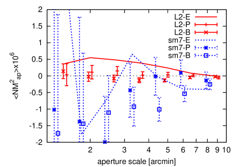
Refer to caption
Figure 14: Plots of 𝒩MMapdelimited-⟨⟩𝒩subscript𝑀perpendicular-tosubscript𝑀ap\langle{\cal N}M_{\perp}M_{\rm ap}\rangle, 𝒩M2delimited-⟨⟩𝒩subscriptsuperscript𝑀2perpendicular-to\langle{\cal N}M^{2}_{\perp}\rangle (L1 low-z𝑧z and sm7 high-z𝑧z) in comparison to the E-mode (lines). Both samples failed the 95% confidence level null test for the P/B-modes, see Table 2.

As indicator of possible systematics in the estimators, we test 𝒩2Mdelimited-⟨⟩superscript𝒩2subscript𝑀perpendicular-to\langle{\cal N}^{2}M_{\perp}\rangle and the combined 𝒩MMapdelimited-⟨⟩𝒩subscript𝑀perpendicular-tosubscript𝑀ap\langle{\cal N}M_{\perp}M_{\rm ap}\rangle, 𝒩M2delimited-⟨⟩𝒩subscriptsuperscript𝑀2perpendicular-to\langle{\cal N}M^{2}_{\perp}\rangle against the null hypothesis. A null measurement should result in a

Δχ2=𝒅tC1𝒅,Δsuperscript𝜒2superscript𝒅tsuperscriptC1𝒅\Delta\chi^{2}={\mn@boldsymbol{d}}^{\rm t}\textbf{{C}}^{-1}{\mn@boldsymbol{d}}\;, (54)

that is statistically consistent with a vanishing signal, with 𝒅𝒅{\mn@boldsymbol{d}} being a vector consisting of the measurements for the P-mode (𝒩2Mapdelimited-⟨⟩superscript𝒩2subscript𝑀ap\langle{\cal N}^{2}M_{\rm ap}\rangle) or both the P- and B-mode (𝒩Map2delimited-⟨⟩𝒩subscriptsuperscript𝑀2ap\langle{\cal N}M^{2}_{\rm ap}\rangle). By C we denote the Jackknife covariance of the measurements as obtained from the variance of B/P-mode measurements in the pointings, as explained in Sect. B.1. This covariance is larger than a null hypothesis covariance as it possibly also contains power from B/P-modes present in the data. A true null model would contain only power from galaxy shape noise and sampling noise. The test results can be found in Table 2. Measurements inconsistent with a null signal (95%percent9595\% confidence) are underlined, thus for Δχ22.0Δsuperscript𝜒22.0\Delta\chi^{2}\geq 2.0 (1.681.681.68) per degree of freedom for 𝒩2Mapdelimited-⟨⟩superscript𝒩2subscript𝑀ap\langle{\cal N}^{2}M_{\rm ap}\rangle (𝒩Map2delimited-⟨⟩𝒩superscriptsubscript𝑀ap2\langle{\cal N}M_{\rm ap}^{2}\rangle). In total, we find two lens samples that fail the test; they are plotted in comparison to their E-mode in Fig. 14. In both cases the failures are related to the 𝒩Map2delimited-⟨⟩𝒩superscriptsubscript𝑀ap2\langle{\cal N}M_{\rm ap}^{2}\rangle statistics and significantly negative B-modes. Note that errors between neighbouring bins are strongly correlated.

Finding two measurements out of in total 57 that fail the 95%percent9595\% test is what we would expect as false positive rate. We therefore conclude that the influence of systematics on the E-mode measurement that reveal themselves via the P- or B-modes is likely to be small compared to our measurement uncertainties. Note that the sm7 sample that failed the null test is not used in the final analysis because the corresponding E-mode signal is consistent with zero.
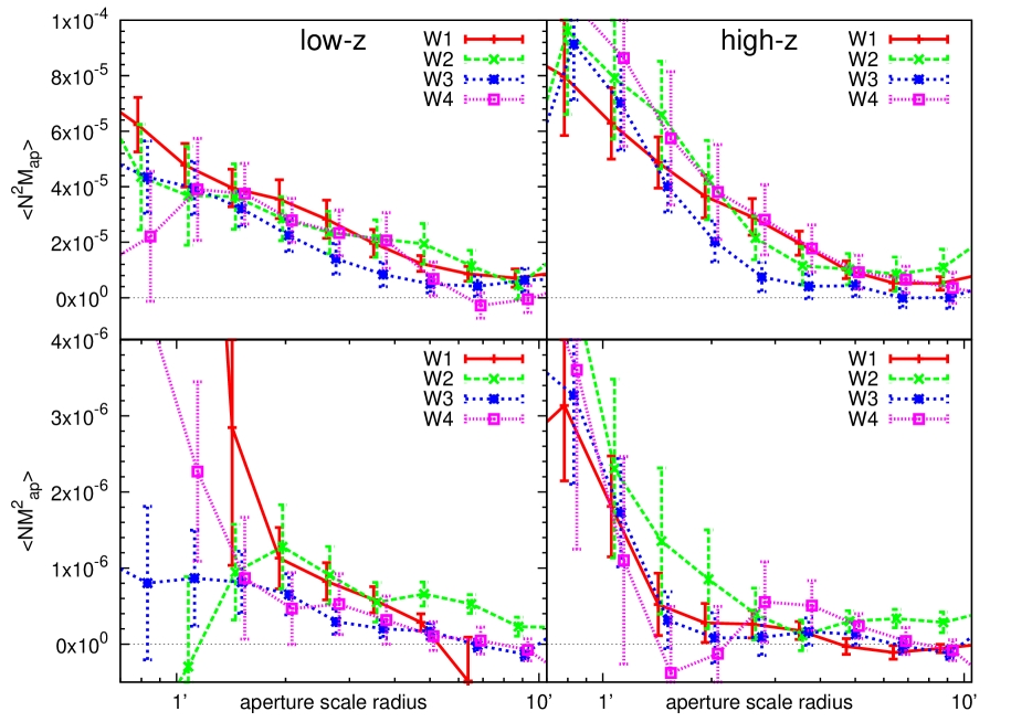
Refer to caption
Figure 15: Measurements of the aperture statistics (top row: 𝒩2Mapdelimited-⟨⟩superscript𝒩2subscript𝑀ap\langle{\cal N}^{2}M_{\rm ap}\rangle, bottom row: 𝒩Map2delimited-⟨⟩𝒩subscriptsuperscript𝑀2ap\langle{\cal N}M^{2}_{\rm ap}\rangle) for the combined L1-L6 sample (low-z𝑧z and high-z𝑧z redshift bin separately). The measurements are split for the four fields W1-W4. The error bars indicate only the pointing-to-pointing variance within the same field. The fields vary in size and thus the sizes of lens and source catalogues vary. Lines connect the data points to guide the eye.

C.2 Field dependence of the G3L signal

The CFHTLS wide survey consists of four contiguous fields W1 (72deg2similar-toabsent72superscriptdeg2\sim 72\,\rm deg^{2}), W2 (33deg2similar-toabsent33superscriptdeg2\sim 33\,\rm deg^{2}), W3 (49deg2similar-toabsent49superscriptdeg2\sim 49\,\rm deg^{2}) and W4 (25deg2similar-toabsent25superscriptdeg2\sim 25\,\rm deg^{2}); the field areas do not include masking or excluded fields due to significant PSF residuals. The fields are well separated on the sky and were observed at different times of the year. By splitting the measurements into W1-W4, we check whether the G3L measurements are comparable for different subsets of the data. To have a possibly large sample for this test, we combine the signals of the samples L1 to L6 for each field, see Fig. 15. Only measurements from pointings within the same fields W1-W4 are combined, their statistical uncertainties originate from the Jackknife technique (as in Eq. 48). Therefore, the error bars do not include the cosmic variance between the fields, which should be most prominent at the larger angular scales.

We find excellent agreement between the measurements, considering that statistical uncertainties at larger scales are higher than indicated and that errors between neighbouring angular bins are correlated. In particular, this separation of data shows that the G3L signal does not originate from singular fields that are extreme outliers compared to the others. Since the uncertainties of the final combined measurements are based on the pointing-to-pointing variance of the entire survey, a possible systematic deviation of one field will be included as systematic error inside the error bars.

Appendix D Third-order galaxy biasing

The values ggmsubscriptggm{\cal B}_{\rm ggm} (mmgsubscriptmmg{\cal B}_{\rm mmg}) measure the u𝑢u-filtered bispectrum B¯ggmsubscript¯𝐵ggm\overline{B}_{\rm ggm} (B¯mmgsubscript¯𝐵mmg\overline{B}_{\rm mmg}), radially smoothed with maximum weight at χmaxsubscript𝜒max\chi_{\rm max}. The maximum weight of the u𝑢u-filter in Fourier space is at k=2/R𝑘2𝑅k=\sqrt{2}/R for a given real space scale R𝑅R. From the definition of the ΨΨ\Psi-statistics, Eq. (5.4), from Eq. (5.3) and from a similar equation for 𝒩Map2delimited-⟨⟩𝒩subscriptsuperscript𝑀2ap\langle{\cal N}M^{2}_{\rm ap}\rangle it follows that

Ψ(R)Ψ𝑅\displaystyle\Psi(R)
=dχd2k1d2k2Fmmg(𝒌1,𝒌2,χ;R)(b3r1)(𝒌1,𝒌2,χ)dχd2k1d2k2Fggm(𝒌1,𝒌2,χ;R)(b32r2)(𝒌1,𝒌2,χ),absentdifferential-d𝜒superscriptd2subscript𝑘1superscriptd2subscript𝑘2subscript𝐹mmgsubscript𝒌1subscript𝒌2𝜒𝑅subscript𝑏3subscript𝑟1subscript𝒌1subscript𝒌2𝜒differential-d𝜒superscriptd2subscript𝑘1superscriptd2subscript𝑘2subscript𝐹ggmsubscript𝒌1subscript𝒌2𝜒𝑅subscriptsuperscript𝑏23subscript𝑟2subscript𝒌1subscript𝒌2𝜒\displaystyle\!\!\!\!\!\!\!=\frac{\int{\rm d}\chi{\rm d}^{2}k_{1}{\rm d}^{2}k_{2}\,F_{\rm mmg}({\mn@boldsymbol{k}}_{1},{\mn@boldsymbol{k}}_{2},\chi;R)\,\left(b_{3}r_{1}\right)({\mn@boldsymbol{k}}_{1},{\mn@boldsymbol{k}}_{2},\chi)}{\int{\rm d}\chi{\rm d}^{2}k_{1}{\rm d}^{2}k_{2}\,F_{\rm ggm}({\mn@boldsymbol{k}}_{1},{\mn@boldsymbol{k}}_{2},\chi;R)\,\left(b^{2}_{3}r_{2}\right)({\mn@boldsymbol{k}}_{1},{\mn@boldsymbol{k}}_{2},\chi)}\;,

where the smoothing kernels in (𝒌,χ)𝒌𝜒({\mn@boldsymbol{k}},\chi)-space are

Fmmg(𝒌1,𝒌2,χ;R)subscript𝐹mmgsubscript𝒌1subscript𝒌2𝜒𝑅\displaystyle F_{\rm mmg}({\mn@boldsymbol{k}}_{1},{\mn@boldsymbol{k}}_{2},\chi;R)
:=qmmg(χ)0χhdχqmmg(χ)×\displaystyle\!\!\!\!:=\frac{q_{\rm mmg}(\chi)}{\int_{0}^{\chi_{\rm h}}{\rm d}\chi\,q_{\rm mmg}(\chi)}\times
u~(k1Λ)u~(k2Λ)u~(|𝒌1+𝒌2|Λ)Bmmm(𝒌1,𝒌2,χ),~𝑢subscript𝑘1Λ~𝑢subscript𝑘2Λ~𝑢subscript𝒌1subscript𝒌2Λsubscript𝐵mmmsubscript𝒌1subscript𝒌2𝜒\displaystyle~{}\tilde{u}(k_{1}\Lambda)\tilde{u}(k_{2}\Lambda)\tilde{u}(|{\mn@boldsymbol{k}}_{1}+{\mn@boldsymbol{k}}_{2}|\Lambda)B_{\rm mmm}({\mn@boldsymbol{k}}_{1},{\mn@boldsymbol{k}}_{2},\chi)\;,
Fggm(𝒌1,𝒌2,χ;R)subscript𝐹ggmsubscript𝒌1subscript𝒌2𝜒𝑅\displaystyle F_{\rm ggm}({\mn@boldsymbol{k}}_{1},{\mn@boldsymbol{k}}_{2},\chi;R)
:=qggm(χ)0χhdχqggm(χ)×\displaystyle\!\!\!\!:=\frac{q_{\rm ggm}(\chi)}{\int_{0}^{\chi_{\rm h}}{\rm d}\chi\,q_{\rm ggm}(\chi)}\times
u~(k1Λ)u~(k2Λ)u~(|𝒌1+𝒌2|Λ)Bmmm(𝒌1,𝒌2,χ)~𝑢subscript𝑘1Λ~𝑢subscript𝑘2Λ~𝑢subscript𝒌1subscript𝒌2Λsubscript𝐵mmmsubscript𝒌1subscript𝒌2𝜒\displaystyle~{}\tilde{u}(k_{1}\Lambda)\tilde{u}(k_{2}\Lambda)\tilde{u}(|{\mn@boldsymbol{k}}_{1}+{\mn@boldsymbol{k}}_{2}|\Lambda)B_{\rm mmm}({\mn@boldsymbol{k}}_{1},{\mn@boldsymbol{k}}_{2},\chi)

with Λ:=RfK(χ)/fK(χmax)assignΛ𝑅subscript𝑓K𝜒subscript𝑓Ksubscript𝜒max\Lambda:=Rf_{\rm K}(\chi)/f_{\rm K}(\chi_{\rm max}). As can be seen, the detailed weight within a band defined by the width of the u𝑢u-filter is also determined by the actual matter bispectrum Bmmmsubscript𝐵mmmB_{\rm mmm}.

We can further exploit the statistical isotropy of the galaxy-matter bispectra, which means that both Bmmmsubscript𝐵mmmB_{\rm mmm} and the galaxy biasing parameters r1,r2,b3subscript𝑟1subscript𝑟2subscript𝑏3r_{1},r_{2},b_{3} are only functions of |𝒌1|,|𝒌2|,ϕsubscript𝒌1subscript𝒌2italic-ϕ|{\mn@boldsymbol{k}}_{1}|,|{\mn@boldsymbol{k}}_{2}|,\phi; ϕitalic-ϕ\phi is the angle spanned by 𝒌1subscript𝒌1{\mn@boldsymbol{k}}_{1} and 𝒌2subscript𝒌2{\mn@boldsymbol{k}}_{2}. The previous expressions therefore simplify to

Ψ(R)Ψ𝑅\displaystyle\Psi(R)
=dχdϕdk1dk2k1k2Fmmg()(b3r1)(k1,k2,ϕ,χ)dχdϕdk1dk2k1k2Fggm()(b32r2)(k1,k2,ϕ,χ),absentdifferential-d𝜒differential-ditalic-ϕdifferential-dsubscript𝑘1differential-dsubscript𝑘2subscript𝑘1subscript𝑘2subscript𝐹mmgsubscript𝑏3subscript𝑟1subscript𝑘1subscript𝑘2italic-ϕ𝜒differential-d𝜒differential-ditalic-ϕdifferential-dsubscript𝑘1differential-dsubscript𝑘2subscript𝑘1subscript𝑘2subscript𝐹ggmsubscriptsuperscript𝑏23subscript𝑟2subscript𝑘1subscript𝑘2italic-ϕ𝜒\displaystyle\!\!\!\!\!\!\!=\frac{\int{\rm d}\chi{\rm d}\phi\,{\rm d}k_{1}{\rm d}k_{2}k_{1}k_{2}\,F_{\rm mmg}(\ldots)\,\left(b_{3}r_{1}\right)(k_{1},k_{2},\phi,\chi)}{\int{\rm d}\chi{\rm d}\phi\,{\rm d}k_{1}{\rm d}k_{2}k_{1}k_{2}\,F_{\rm ggm}(\ldots)\,\left(b^{2}_{3}r_{2}\right)(k_{1},k_{2},\phi,\chi)}\;,

where

Fmmg()subscript𝐹mmg\displaystyle F_{\rm mmg}(\ldots)
:=qmmg(χ)0χhdχqmmg(χ)×\displaystyle\!\!\!\!:=\frac{q_{\rm mmg}(\chi)}{\int_{0}^{\chi_{\rm h}}{\rm d}\chi\,q_{\rm mmg}(\chi)}\times
u~(k1Λ)u~(k2Λ)u~(|𝒌1+𝒌2|Λ)Bmmm(k1,k2,ϕ,χ),~𝑢subscript𝑘1Λ~𝑢subscript𝑘2Λ~𝑢subscript𝒌1subscript𝒌2Λsubscript𝐵mmmsubscript𝑘1subscript𝑘2italic-ϕ𝜒\displaystyle~{}\tilde{u}(k_{1}\Lambda)\tilde{u}(k_{2}\Lambda)\tilde{u}(|{\mn@boldsymbol{k}}_{1}+{\mn@boldsymbol{k}}_{2}|\Lambda)B_{\rm mmm}(k_{1},k_{2},\phi,\chi)\;,
Fggm()subscript𝐹ggm\displaystyle F_{\rm ggm}(\ldots)
:=qggm(χ)0χhdχqggm(χ)×\displaystyle\!\!\!\!:=\frac{q_{\rm ggm}(\chi)}{\int_{0}^{\chi_{\rm h}}{\rm d}\chi\,q_{\rm ggm}(\chi)}\times
u~(k1Λ)u~(k2Λ)u~(|𝒌1+𝒌2|Λ)Bmmm(k1,k2,ϕ,χ),~𝑢subscript𝑘1Λ~𝑢subscript𝑘2Λ~𝑢subscript𝒌1subscript𝒌2Λsubscript𝐵mmmsubscript𝑘1subscript𝑘2italic-ϕ𝜒\displaystyle~{}\tilde{u}(k_{1}\Lambda)\tilde{u}(k_{2}\Lambda)\tilde{u}(|{\mn@boldsymbol{k}}_{1}+{\mn@boldsymbol{k}}_{2}|\Lambda)B_{\rm mmm}(k_{1},k_{2},\phi,\chi)\;,

and

|𝒌1+𝒌2|=k12+k22+2k1k2cosϕ.subscript𝒌1subscript𝒌2superscriptsubscript𝑘12superscriptsubscript𝑘222subscript𝑘1subscript𝑘2italic-ϕ|{\mn@boldsymbol{k}}_{1}+{\mn@boldsymbol{k}}_{2}|=\sqrt{k_{1}^{2}+k_{2}^{2}+2k_{1}k_{2}\cos{\phi}}\;. (59)

Note that for equilateral triangles we have k1=k2=|𝒌1+𝒌2|subscript𝑘1subscript𝑘2subscript𝒌1subscript𝒌2k_{1}=k_{2}=|{\mn@boldsymbol{k}}_{1}+{\mn@boldsymbol{k}}_{2}| and thus cosϕ=1/2italic-ϕ12\cos{\phi}=-1/2.