Polarons on one-dimensional lattice.
II. Moving polaron.

Abstract

In the present study we revise the possible polaron contribution to the charge and energy transfer over long distances in biomolecules like DNA. The harmonic and the simple inharmonic ($U(x)=x^{2}/2-\beta x^{3}/3$) lattices are considered. The systems of PDEs are derived in the continuum approximation. The PDEs have the one-soliton solution for polarons on the harmonic lattice. It describes a moving polaron, the polaron velocity lies in the region from zero to the sound velocity and depends on the polaron amplitude. The PDEs describing polarons on the inharmonic lattice also have the one-soliton solution only in the case of special relation between parameters (parameter of inharmonicity $\beta$ and parameter of electron-phonon interaction $\alpha$). Polaron dynamics is numerically investigated in the wide range of parameters, where the analytical solutions are not available. Supersonic polarons are observed on inharmonic lattice with high inharmonicity. There is the range of parameters $\alpha$ and $\beta$ where exists a family of unusual stable moving polarons with the envelope consisting of several peaks (polarobreather solution). The results are in qualitative agreement with recent experiments on the charge transport in DNA.

Keywords: polaron, charge transport, DNA

PACS numbers: 71.38.-k; 87.15.-v

I Introduction

This paper continues our investigations on the polarons in 1D lattices Lik12 . Its primary goal is an explanation of the high efficient charge transfer in biological macromolecules.

Charge transfer (CT) is of utmost importance in physics, chemistry and biology Bar96 ; Bix99 ; Ber04 ; Mat02 ; Ada03 ; Wei05 ; Gen10 ; Mal10 ; Shi10 ; Kuz95 ; Kuz99 ; Bal01 . For instance, it is essential in processes at nano– and micro–scales, for solar cells technology Was92 , molecular electronics Rat97 ; Lin07 and other novel technologies. The CT is very important, e.g. for oxidative DNA degradation Sch04 . Noteworthy is that DNA has been labelled as electric conductor Fin99 , semiconductor Por00 , insulator Ber97 and even superconductor Kas01 . Such wide range of possible electric properties is explained by the variety of different DNA structures used, diversity of experimental methods and inner and outer surrounding DNA conditions. It has been shown that the rate of CT exponentially decays with the distance $L$ as $k_{\rm CT}\propto\exp(-\gamma L)$, where $\gamma\gtrsim 0.1-0.2$ Å^-1 Tak04 ; Lew06a ; Lew06b .

Significant progress in enhancing the conducting properties of DNA was achieved after the DNA synthesis reached its present status of automation. Apparently adenine (A) is the most preferable building block because of its resistance to charge trapping Lew01 and its CT efficiency Nei04 ; Sha05 . Three sets of duplexes were synthesized giving 4–, 6– and 14–base A tracts with a covalently attached rhodium complex [Rh(phi)₂(bpy^′)]³⁺ serving as the photooxidant Aug07 . It was found that there was no significant change in degree of decomposition ($\gamma=0.0013$ Å^-1), i.e. the efficiency of charge transport very slowly depends on the distance, what contrasts with the larger values found in previous experiments. The possibility of CT over 34 nm (100-mer DNA) was recently announced by J. Barton and collaborators Sli11 and this result surpasses most previous achievements with molecular wires.

Analogous results were obtained for the synthetic $\alpha$-helical peptides where a very shallow distance dependence of the charge transfer was also found Ari10 . One interesting feature in these studies was revealed: the charge transport is a coherent single-step process, i.e. the charge carrier can be transferred ballistically Gen11 ; Bar11 .

Traditionally the hopping and tunnelling are considered as a most abundant mechanisms in the theory of charge transfer in DNA Wag05 ; Sch04a ; Sch04b ; Cha07 . Polarons were also extensively studied as candidates for charge carriers Con01 ; Con00 ; Con05 ; Kuc10 ; Mah10 ; Wu-11 ; Feh11 ; Man03 (see also review Dev09 ). At present, the polaron theory of CT in biomacromolecules is very popular. Polarons are considered in different models and approximations Kuc10 ; Kal98 ; Sch10 ; Kub10 ; Lak10 ; Lak05 ; Hen04 ; Hen06 ; Yam07 .

Effects of nonlinearity can give contribution to the charge transport due to formation of the bounded soliton–electron state Zol93 ; Zol96 or polarobreathers Aub97 ; Cru00 ; Cue06 ; Fla98 ; Hen00 ; Hen03 ; Kal04 ; Kal05 ; Yu-04 . As a working definition breathers are localized solutions with at least two degrees of freedom in a one-dimensional lattice (i.e., they have an ‘‘internal’’ degree of freedom, a vibrational motion) while stable localized solutions with one degree of freedom are solitons Cru00 .

Recently the concept of nonlinearity was additionally advanced and solectrons, – bounded state of solitons and charge carriers, were found in numerical experiments (see Vel10 and references therein).

Notably, the charge transfer in DNA appearers to be independent of distance but is critically sensitive to different kinds of defects, – static and dynamical disorder Boo00 ; Zha04 . Biomacromolecules are very complex systems and many kinds of fluctuations can disturb the path-ways of charge migration. A DNA macromolecule is supposed to have a uniform or a random distribution of the helix angles. And an influence of angles fluctuations on the charge transfer efficiency was analyzed Qua08 ; Cra05 ; Yu-01 ; Bru00 . Dynamical fluctuations (temperature) also can affect the hopping probability thus giving rise to charge localization Con00 ; Kat02 ; Qu-10 ; Qua09 .

In the present paper we consider the charge transport in harmonic and inharmonic lattices and derive analytical expressions for moving polarons in the continuum approximation. Polaron dynamics is investigated numerically in the range of parameters where the analytical solutions are not available. Special attention is given to possible explanation of recent experiments on the charge transport in DNA.

II Moving polaron on the harmonic lattice

We start from consideration of 1D harmonic lattice with free boundaries consisting of $N$ particles with the hamiltonian

$$H=\dfrac{m}{2}\sum\limits_{j=1}^{N}\dot{x}_{j}^{2}+\dfrac{k}{2}\sum\limits_{j=1}^{N-1}(x_{j+1}-x_{j})^{2}+\left<\vec{\Psi}\,|\widehat{H}^{\rm e}|\,\vec{\Psi}\right>,$$ (1)

where $\vec{\Psi}=\psi_{1},\psi_{2},\ldots,\psi_{N}$ is the discrete wave function, $m$ is the particle mass, $k$ is the lattice rigidity, $x_{j}$ is deviation of the $j$th particle from the equilibrium. ‘‘Particle’’ represents the DNA base, and their interaction is due to the $\pi-\pi$ overlapping of neighboring heteroaromatic bases.

The components of the electron-phonon interaction operator are:

$$H_{i,j}^{\rm e}=\delta_{j,j}e_{j}+\delta_{j,j-1}t_{j-1}+\delta_{j,j+1}t_{j},$$ (2)

where $\delta_{i,j}$ is the Kronecker symbol; $t_{j}$ – hopping integral between $j$th and $(j+1)$th particles; $e_{j}$ is the energy of interaction of the charge carrier with the lattice site (on-site energy). This strategy is known as the tight-binding approach to DNA which takes into account the on-site energies and suitably parametrized hopping onto the neighboring sites Con00 ; Con05 ; Cun07 .

The main object of the present investigation is synthetic DNA comprised of identical base pairs. So the diagonal disorder is absent and $e_{i}=$ const. This constant is the electronic energy origin and without the loss of generality can be put to zero. The hopping integral is often written in the form suggested by Su, Schrieffer and Heeger Su-79 ; Su-80 :

$$t_{j}=-[v_{0}-\alpha(x_{j+1}-x_{j})]\,,$$ (3)

where $v_{0}$ is the hopping integral at the equilibrium and parameter $\alpha$ accounts the electron-phonon interaction. The electron charge transfer is considered, though all results are valid for the hall transfer.

It is convenient to make hamiltonian (1) dimensionless using mass $m$, energy $v_{0}$ and the rigidity coefficient $k$ as the units. Then the unit of time $[t]=\sqrt{m/k}$, unit of length $[L]=\sqrt{v_{0}/k}$. If the DNA parameters are chosen Con00 ; Con05 , namely $v_{0}=0.3$ eV, $k=0.85$ eV/Ų, $m=130$ a.m.u., then the time unit is $(t)\approx 0.13$ ps, and the length unit is $[L]\approx 0.59$ Å. Parameter $\alpha$ is also dimensionless: $\alpha/\sqrt{v_{0}k}\to\alpha$. The dimensionless value of this parameter for DNA $\alpha\approx 1.2$. Parameter $\alpha$ is the single parameter specifying the lattice.

The dimensionless hamiltonian (1) reads:

$$H=\dfrac{1}{2}\sum\limits_{j=1}^{N}\dot{x}_{j}+\dfrac{1}{2}\sum\limits_{j=1}^{N-1}q_{j}^{2}-\sum\limits_{j=1}^{N-1}(1-\alpha q_{j})\,(\psi_{j}^{*}\psi_{j+1}+{\rm c.c.})\,,$$ (4)

where $q_{j}\equiv(x_{j+1}-x_{j})$ is the relative displacement of neighboring particles. This hamiltonial together with the Schrödinger equation $i\hbar\vec{\Psi}=\widehat{H}^{\rm e}\vec{\Psi}$ generates the system of evolution equations:

$$\left\{\begin{split}\ddot{x}_{j}=&(q_{j}-q_{j-1})-\alpha[(\psi_{j}^{*}\psi_{j+1}+{\rm c.c.})-(\psi_{j-1}^{*}\psi_{j}+{\rm c.c.})]\\ \dot{\psi}_{j}=&\dfrac{i}{\widetilde{h}}\left[(1-\alpha q_{j-1})\psi_{j-1}+(1-\alpha q_{j})\psi_{j+1}\right],\end{split}\right.$$ (5)

where $\widetilde{h}$ is the dimensionless Planck’s constant: $\dfrac{\hbar}{v_{0}}\sqrt{\dfrac{k}{m}}\to\widetilde{h}\approx 0.017$.

The evolution equations in variables $q_{j}$ and $\psi_{j}$ are

$$\left\{\begin{split}\ddot{q}_{j}=&(q_{j+1}-2q_{j}+q_{j-1})-\alpha[(\psi_{j+1}^{*}\psi_{j+2}+{\rm c.c.})-2(\psi_{j}^{*}\psi_{j+1}+{\rm c.c.})+(\psi_{j-1}^{*}\psi_{j}+{\rm c.c.})]\\ \dot{\psi}_{j}=&\dfrac{i}{\widetilde{h}}\left[(1-\alpha q_{j})\psi_{j+1}+(1-\alpha q_{j-1})\psi_{j-1}\right].\end{split}\right.$$ (6)

Eqs. (6) are more useful for analytical consideration, while Eqs. (5) are more suitable for numerical calculations.

Eqs. (6) can be reduced to the system of continuous equations in the long-wave approximation. Let us expand the variables $g_{j}$ and $\psi_{j}$ into Taylor series:

$$\begin{split}q_{j\pm 1}=&\,q_{j}\pm\epsilon q_{j}^{\prime}+\epsilon^{2}\dfrac{1}{2}q_{j}^{\prime\prime}\pm\ldots\\ \psi_{j\pm 1}=&\,\psi_{j}\pm\epsilon\psi_{j}^{\prime}+\dfrac{1}{2}\epsilon^{2}\psi_{j}^{\prime\prime}\pm\ldots\end{split}$$ (7)

where $\epsilon$ is small parameter. After substitution of Eqs. (7) into Eqs.(6) one can get the system of nonlinear partial differential equations (PDEs):

$$\left\{\begin{split}q_{tt}=&q_{xx}+2\alpha(\psi\psi^{*})_{xx}\\ \psi_{t}=&\dfrac{i}{\widetilde{h}}[2(1-\alpha q)\,\psi+\psi_{xx}]\,,\end{split}\right.$$ (8)

where terms of the order $\epsilon^{3}$ and higher are omitted. This system is not integrable, but it has special one-soliton solution:

$$\left\{\begin{split}q(x,t)=&-\dfrac{A}{\cosh^{2}[d(x-v_{\rm p}t)]}\\ \psi(x,t)=&\dfrac{B\,\exp[i(kx+\omega t)]}{\cosh[d(x-v_{\rm p}t)]}\,,\end{split}\right.$$ (9)

where $1/d$ is the polaron width and $v_{\rm p}$ is the polaron velocity. $A,B$ are amplitude of relative displacements and amplitude of the wave function, correspondingly, $(kx+\omega t)$ is the phase of the wave function. If $v_{\rm p}=0$ then (9) coincides with the solution for the unmovable polaron Lik12 .

Solution (9) is the one-parametric solution with the following relation between parameters:

$$d=\sqrt{\alpha A};\quad v_{\rm p}=\left(1-\sqrt{\dfrac{\alpha^{3}}{A}}\right)^{1/2}\approx 1-\dfrac{1}{2}\sqrt{\dfrac{\alpha^{3}}{A}};\quad B=\sqrt{\dfrac{d}{2}}.$$ (10)

and

$$k=\dfrac{\widetilde{h}v_{\rm p}}{2}\ll 1;\qquad\omega=\dfrac{2+d^{2}-k^{2}}{\widetilde{h}}\gg 1\,.$$ (11)

and the amplitude of relative displacements $A$ can be chosen as a free parameter specifying the polaron. Other parameters ($d,\,v_{\rm p}$) are defined through amplitude $A$. The norm of the wave function $\int\limits_{-\infty}^{\infty}|\psi(x)|^{2}{\rm d}x=1$ was preserved while deriving (10)–(11).

The polaron velocity $v_{\rm p}$ lies in the range from zero (unmovable polaron) to the sound velocity (the dimensionless sound velocity $v_{\rm snd}=1$). The amplitude of the moving polaron $A\geq A_{\rm min}$ and $A_{\rm min}=\alpha^{3}$ is the amplitude of unmovable polaron.

Now we check the analytical results in numerical simulation of Eqs. (5). First of all we find the range of parameter $\alpha$ where the continuous approximation is valid. Fig. 1a shows the dependence of the unmovable polaron amplitude vs. parameter $\alpha$ of the electron-phonon interaction. Analytical and numerical results coincide for $\alpha\lesssim 0{.}4$.

Fig. 1b shows the dependence of polaron velocity vs. its amplitude $A$ for two values of parameter $\alpha$. As expected, coincidence is very good for $\alpha=0.4$ and there is some disagreement for larger values of $\alpha$. But despite some discrepancy for $\alpha=0{.}7$, the numerical data form a distinct dependence. It means that there can exists the polaron solution of (6) which, nevertheless, is not governed by the continuum approximation.

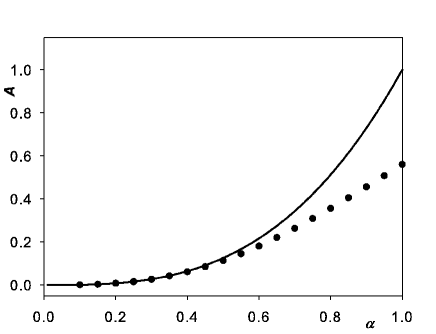
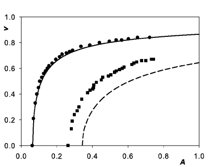
a)                                                                       b)

Figure 1: (a) Dependence of the unmovable polaron amplitude $A$ vs. parameter $\alpha$. Solid line is analytical prediction, dots are results of numerical simulation. (b) Dependence of the polaron velocity $v$ vs. the amplitude $A$ for two values of parameter $\alpha$. Analytical results (10) are shown by solid ($\alpha=0.4$) and dashed ($\alpha=0.7$) lines. Numerical results are shown by circles ($\alpha=0.4$) and squares ($\alpha=0.7$).

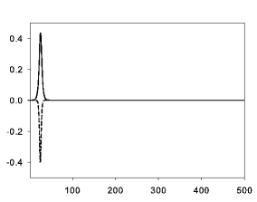
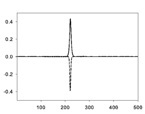
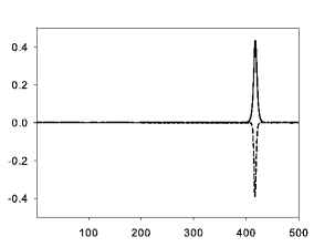
a)                                         b)                                         c)

Figure 2: Snapshots of the polaron evolution on the harmonic lattice at different time moments: $t=0$ (a), $t=250$ (b) and $t=500$ (c). Polaron is centered on the site $j_{0}=25$ at $t=0$. Positive values along the ordinate axis are the modulus of wave function $|\psi_{j}|$ (solid line), and negative values are relative displacements (dashed line). Lattice parameters are $\alpha=0{.}4$, $N=500$. Initial polaron amplitude $A=0{.}4$.

We use parameter $\alpha=0.4$ for the analysis of the polaron stability. Figs. 2 demonstrates high polaron stability, where snapshots of the polaron evolution are shown at three time moments. The initial conditions are chosen according to (9)-(11) for $A=0.4$. The polaron is very stable, it travels $\approx 400$ lattice sites without any noticeable change. The calculated polaron velocity ($v_{\rm p}\approx 0.78$) is in good agreement with analytical prediction ($v_{\rm anal}=0.775$).

The polaron initially generated according to the ‘‘correct’’ initial conditions is very stable. The problem is whether the polaron can be formed and is it stable in the case of arbitrary initial conditions? To answer this question the initial excitation is chosen according to (9)-(11) for $A=0{.}4$, but the velocity is $v_{\rm p}=0{.}2$ instead of correct value $v_{\rm anal}=0{.}775$. The evolution of this initial state is shown in Fig. 3. Stable polaron with parameters $A\approx 0{.}21,\,\,v_{\rm p}\approx 0{.}68$ forms soon (polarons in Figs. 3b and 3c are practically identical). The polaron amplitude decreased relative to initial value. But relations (10) and (11) are fulfilled for parameters of this polaron with high accuracy, i.e. the analytical polaron velocity $v_{\rm anal}\approx 0.67$ for the polaron amplitude $A=0.21$. The initial excitation transforms into polaron accompanied by the noise irradiation. Noteworthy, that 100% of the electron wave function is localized at polaron; no fraction of the wave function is irradiated with the noise.

Wide range of initial conditions was tested and in all cases stable polaron is formed with the relations between parameters obeying (10)–(11).

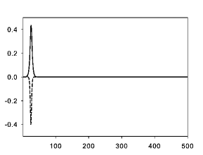
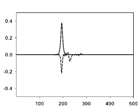
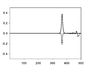
a)                                         b)                                         c)

Figure 3: Polaron evolution with initial conditions: $\alpha=0.4,\,A=0.4$ and polaron velocity $v_{p}=0.2$ which does not satisfy correct relations (10). Snapshots are shown at $t=0,\,\ t=250$ and $t=500$. Lines and axes are the same as in Fig. 2. $N=500$.

In the next section we transform Eqs. (8) into the integrable system of PDEs.

III Reduction to the integrable system of partial
differential equations.

Let us rewrite system (8) for convenience:

$$\left\{\begin{split}q_{tt}=&q_{xx}+2\alpha(\psi\psi^{*})_{xx}\\ \psi_{t}=&\dfrac{i}{\widetilde{h}}[2(1-\alpha q)\,\psi+\psi_{xx}]\,.\end{split}\right.$$ (12)

We follow the reductive perturbation method (RPM) Sas81 ; Leb08 where a special variable transformation

$$\left\{\begin{split}q=\,&\varepsilon u_{1}+\varepsilon^{2}u_{2}+\ldots\\ y=\,&\varepsilon^{1/2}(x-c\,t)\\ \tau=\,&\varepsilon^{3/2}t,\end{split}\right.$$ (13)

is made and $\varepsilon$ is small parameter. The main objective of the RPM usage is the reduction of the degree of derivative by time $q_{tt}$ in (12) to the first order. The new (laboratory) coordinate system moves with velocity $c$ relative to the old coordinate system (second line in (13) ).

Substituting (13) into (12) and equating terms of the order $\varepsilon^{2}$ one gets that $c=1$. It means that the laboratory coordinate system moves with the sound velocity $c=v_{\rm snd}=1$ relative to the old coordinate system.

Equating terms of the order $\epsilon^{3}$ and taking into account that the solution tends to zero at $\pm\infty$, we get

$$\left\{\begin{split}{}&2u_{\tau}=2\alpha(\psi\psi^{*})_{y}\\ {}&i\widetilde{h}(\psi_{\tau}-\psi_{y})=-2(1-\alpha u)\psi-\psi_{yy}.\end{split}\right.$$ (14)

Additional linear variables transformation ($\psi(y,\tau)=\widetilde{a}\,\Psi(z,T)\,\exp[i(\widetilde{k}z-\widetilde{\omega}T)],\,\,u(y,\tau)=\widetilde{b}\,U(z,T),\,\,\tau=\widetilde{c}\,T,\,\,y=\widetilde{d}z$) is necessary to reduce (14) to the ‘‘standard’’ form:

$$\left\{\begin{split}U_{T}=&\,2(\Psi\Psi^{*})_{z}\\ i\Psi_{T}=&\,U\Psi+\Psi_{zz},\end{split}\right.$$ (15)

where coefficients labelled with ‘tilde’ are some linear combinations of ‘‘old’’ coefficients.

System (15) is exactly solvable and its one-, two-soliton etc. solutions are known Dub88 . As a particular case, the one-soliton solution has the same functional form as solution (9). But the relation between parameters $A,\,B,\,d,\,v_{\rm p}$ is somewhat different. Numerical simulation confirms high stability of polarons described by the solution of (15).

The numerical experiments of polaron interaction shows that the polarons preserve their shapes after collision. This fact additionally proves the fact that integrable system (15) is a good approximation for discreet system (6).

In the next section we consider the moving polaron on the inharmonic lattice.

IV Moving polaron on the inharmonic lattice

In this section we consider the inharmonic lattice with the dimensionless FPU potential:

$$U(q)=\dfrac{1}{2}q^{2}-\dfrac{\beta}{3}q^{3},$$ (16)

where $\beta$ is the parameter of non-linearity and $q$ is the relative displacement of particles. Many realistic potentials (Morse, Lennard-Jones, etc) are reduced to (16) when the deviations from equilibrium are not large (the expansion of potentials into the Tayler series up to the third order). Moreover, the $\alpha$-FPU potential (16) allows to make necessary analytical calculus.

We employ the same procedure as in the case of harmonic potential. We expand the relative displacements and the wave function into Taylor series according to (7). The result is the system of PDEs:

$$\left\{\begin{split}q_{tt}=&\left(q_{xx}+\dfrac{1}{12}q_{xxxx}\right)-\beta\left(q^{2}\right)_{xx}+2\alpha\left(\psi\psi^{*}\right)_{xx};\\ \psi_{t}=&\dfrac{i}{\widetilde{h}}[2(1-\alpha q)\,\psi-\psi_{xx}].\end{split}\right.$$ (17)

Unfortunately, the relation between coefficients in (17) is such, that this system can not be reduced to the exactly solvable PDEs Dub88 which has the canonical form:

$$\left\{\begin{split}3u_{tt}=&(u_{xxx}-6u\,u_{x})_{x}+8|\phi|^{2}_{xx};\\ i\,\phi_{t}=&\phi_{xx}-u\phi.\\ \end{split}\right.$$ (18)

However, if $\beta=2\,\alpha$ (coefficients of the second spatial derivatives in the first equation in (17) are equal), then system (17) has the special one-soliton solution. This solution has the same form as for the harmonic lattice:

$$\left\{\begin{split}q(x,t)=&-\dfrac{A}{\cosh^{2}[d(x-vt)]}\\ \psi(x,t)=&\dfrac{B\,\exp[i(kx+\omega t)]}{\cosh[d(x-vt)]}\end{split}\right.$$ (19)

with the relations between parameters:

$$\begin{array}[]{l}d=\sqrt{\alpha A}=\sqrt{2\beta A},\\ v_{\rm p}=\left(1-\sqrt{\dfrac{\alpha^{3}}{A}}+\dfrac{\beta A}{3}\right)^{1/2}\approx 1-\dfrac{1}{2}\sqrt{\dfrac{\alpha^{3}}{A}}+\dfrac{\beta A}{6},\\ B=\sqrt{\dfrac{d}{2}}\end{array}$$ (20)

and

$$k=\dfrac{\widetilde{h}v_{\rm p}}{2}\ll 1;\qquad\omega=\dfrac{2+d^{2}-k^{2}}{\widetilde{h}}\gg 1.$$ (21)

There is an addition term in the expression for the polaron velocity (20) as compared to the polaron velocity on the harmonic lattice (10). This positive term is due to the nonlinearity, and the actual velocity is determined by the balance of electron-phonone interaction and nonlinearity. In the absence of the electron-phonon interaction ($\alpha=0$) the velocity is $v\approx 1+\beta A/6$, and is the soliton velocity on the $\alpha$-FPU lattice Rem03 .

Now we verify the polaron stability in numerical simulations on the inharmonic lattice in a way analogous to the harmonic lattice. Fig. 4a shows the dependence of the unmovable polaron amplitude vs. the parameter $\alpha$ of the electron-phonon interaction. One can see, that there is also a good agreement between analytical and numerical results for $\alpha\lesssim 0{.}4$.

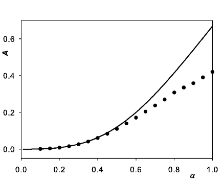
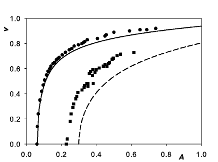
a)                                                                       b)

Figure 4: (a) The dependence of the polaron amplitude vs. parameter $\alpha$ for the unmovable polaron. Solid line is analytical solution (19) with parameters (20)–(21), dots are numerical results. (b) Dependence of the polaron velocity vs. amplitude $A$ for two values of parameter $\alpha$: $\alpha=0{.}4$ (solid line is analytical dependence, circles are numerical results), $\alpha=0{.}7$ (dashed line is analytical dependence, squares are numerical results).

Figure 4b shows the dependence of the polaron velocity vs. amplitude $A$ of relative displacements for two value of parameter of electron-phonon interaction $\alpha$. A good agreement between analytical and numerical results is also observed for $\alpha=0{.}4$ but there is some gap for $\alpha=0{.}7$. Similar to the harmonic lattice, the numerical data form a well-defined dependence for $\alpha=0{.}7$. It means that there can exist polarons which are not governed by the continuum approximation.

Numerical simulations show high polaron stability. Figs. 5 illustrates snapshots of the polaron evolution at three time moments, when the initial conditions are generated according to (19)–(21). The initial polaron amplitude is $A=0{.}3$. The polaron preserves initial parameters in the course of the evolution. The calculated polaron velocity is $v_{\rm p}\approx 0{.}78$, whereas the analytical velocity $v_{\rm anal}=0{.}76$ for $A=0{.}3$.

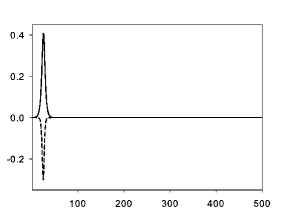
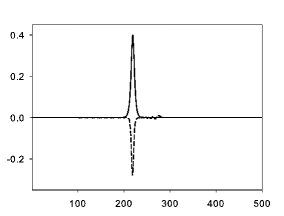
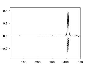
a)                                         b)                                         c)

Figure 5: Snapshots of the polaron evolution on inharmonic lattice ($\alpha=0{.}4$, $\beta=0.2$) at different time moments: $t=0$ (a), $t=250$ (b) and $t=500$ (c). The polaron is centered on the site $j_{0}=25$ at $t=0$, the initial polaron amplitude $A=0{.}3$. Positive values along the ordinate axes are modulus of the wave function $|\psi_{j}|$ (solid line), negative values are relative displacements $q_{j}$ (dashed line).

The polaron evolution with improper initial conditions is shown in Figs. 6. The initial polaron is formed according to Eqs.(19)-(21), but the polaron velocity is chosen to be $v_{\rm p}=0{.}2$ instead of analytically predicted $v_{\rm anal}=0{.}76$. The simulation show that the polaron self-organizes (compare polarons in Figs. 6b and 6c). Parameters of self-organized polaron satisfy (20)–(21) with high accuracy. The ‘‘numerical’’ polaron has velocity and amplitude $v_{\rm p}\approx 0{.}65$ and $A\approx 0{.}16$ whereas $v_{\rm anal}=0{.}63$ if $A=0{.}16$ for the ‘‘analytical’’ polaron.

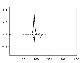
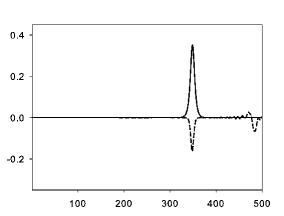
a)                                         b)                                         c)

Figure 6: Polaron evolution with improper initial conditions. Snapshots are shown at $t=0$ (a), $t=250$ (b) and $t=500$ (c). Notation and axes are the same as in Fig. 5

The numerical simulations show that polaron is stable on the inharmonic lattice. However, the results demonstrated above are valid only if $\alpha=2\,\beta$ and $\alpha\lesssim 0{.}4$. In this case the lattice inharmonicity is small ($\beta=0{.}2$) and does not influences essentially on the polaron evolution. The case of large $\alpha$ and $\beta$ are of greater interest. This case is considered numerically in the next Section.

V Numerical simulation on the nonlinear lattice
with arbitrary parameters

Equations

$$\left\{\begin{split}\ddot{x}_{j}=&(q_{j}-q_{j-1})+\beta(q_{j-1}^{2}-q_{j}^{2})-\alpha[(\psi_{j}^{*}\psi_{j+1}+{\rm c.c.})-(\psi_{j-1}^{*}\psi_{j}+{\rm c.c.})],\\ \dot{\psi}_{j}=&\dfrac{i}{\widetilde{h}}\left[(1-\alpha q_{j-1})\psi_{j-1}+(1-\alpha q_{j})\psi_{j+1}\right];\qquad q_{j}\equiv x_{j+1}-x_{j}\end{split}\right.$$ (22)

are integrated numerically with different initial conditions. We use initial conditions in the form (19), but $A$, $d$, $v$ are arbitrary parameters and $k=0$. The question is whether polarons are really exist in the case when the continuous approximation is not valid.

Fig. 7 illustrates how the strange four-peaked polaron-like excitation self-organizes on the inharmonic lattice with parameters $\alpha=0.4$, $\beta=1.0$. The polaronic nature of this excitation is supported by the 100% bearing of the wave function by the localized lattice compression. Initial excitation at $t=0$ is chosen with parameters $d=0.1$, $A=0.6$, $v_{\rm p}=0.7$, $k=0$. Lattice excitations behind the polaron do not have the electronic components and are solitons. The linear relation between soliton velocities and amplitudes Rem03 is clearly visible in Fig. 7 and additionally supports the solitonic nature of these excitations. This numerical simulation is an example of how an arbitrary initial conditions transform to the polaron with extra perturbations emitted in the forms of polaron. Noteworthy that there are no fluctuating lattice vibrations.

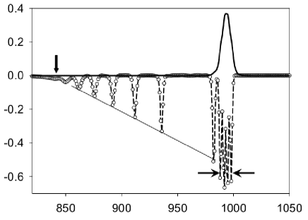
Figure 7: The result of the evolution of the initial excitation at $t=800$. The formed polaron is indicated by two arrows for clarity. There are six solitons behind the polaron. The front of the sound propagation is shown by the vertical arrow. The initial excitation is centered at $j_{0}=50$. Modulus of the wave function – solid line; relative lattice displacements – dashed line. $N=1200$.

To verify the stability of the obtained four-peaked polaron, we use it parameters ($x_{j},\,v_{j},\,\psi_{j};\,j=980\div 1020$), located between two horizontal arrows in Fig. 7, as the initial condition for new numerical simulation. The result of evolution is shown in Fig. 8. The polaron is very stable. After travelling through $\approx\!400$ lattice sites its parameters are not changed and it moves with constant supersonic velocity $v_{\rm p}\approx 1{.}14$.

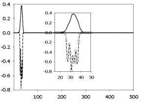
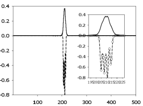
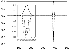
a)                                         b)                                         c)

Figure 8: The evolution of the four-peaked polaron formed from the initial conditions of previous numerical experiment. Inserts show polarons with higher resolution. $N=500$.

The most natural and expected shape of the polaron envelope is a smooth bell-shaped form and an existence of four-peaked polaron is quite unexpected. But there exist polarons with other number of peaks.

Fig. 9 shows how the two-peaked polaron self-organizes. The initial excitation is chosen more narrow than in the previous numerical experiment. The initial parameters are $d=0.5$, $A=0.6$, $v_{\rm p}=0.7$, $k=0$. The evolution of this initial state is more complex: there are intermediate one–, two– and three-peaked excitations. And finally, after rather long time, the two-peaked polaron becomes the stable state. Its velocity is somewhat less then the sound velocity. Numerical simulations show that other initial conditions can produce three-peaked polarons.

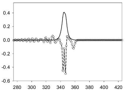
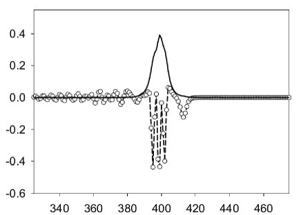
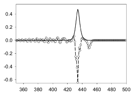
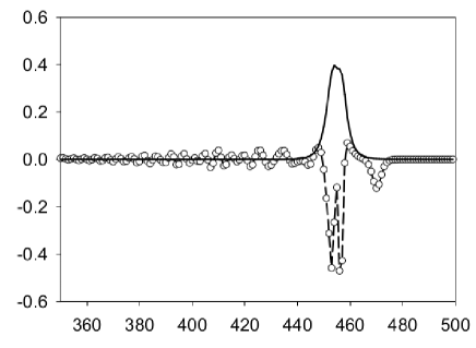
a)                                                                       b) c)                                                                       d)

Figure 9: The snapshots of the polaron at different time moments: $t=321$ (a), $t=345$ (b),$t=380$ (c), $t=400$ (d).

And finally we consider the inharmonic lattice with parameters $\alpha$ and $\beta$ corresponding to the parameters in DNA. Usually the Morse potential is used to account the interaction of neighboring bases $U(q)=D[1-\exp(-bq)]^{2}$. An expansion of this potential into the Taylor series gives the $\alpha$-FPU potential. In the dimensionless form the potential is $U(q)\approx\dfrac{1}{2}q^{2}-\dfrac{\beta}{3}q^{3}$ with $\beta\approx 1.1$ and $\alpha\approx 1.2$.

This set of parameters does not allow an analytical consideration. Numerical simulations are carried out for wide range of initial conditions. As an examples the evolution with different initial parameters are analyzed. Results are shown in Fig. 10. Polarons self-organize from all used initial conditions. But no multi-peaked polarons are found at these parameters choice.

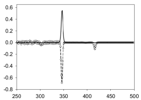
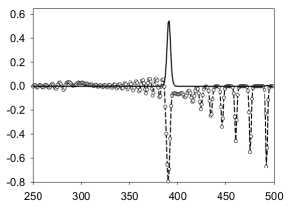
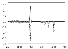
a)                                         b)                                         c)

Figure 10: The result of evolution of the excitation with different initial parameters at $t=350$: $A=0.6,\,\,d=0.4,\,\,v_{\rm p}=1.0$ (a); $A=0.6,\,\,d=0.1,\,\,v_{\rm p}=1.2$ (b); $A=0.5,\,\,d=0.2,\,\,v_{\rm p}=0.5$ (c). Lattice parameters: $N=500$, $\alpha=1.2$, $\beta=1.1$.

The obtained results are rather unusual. First, the polaron can be supersonic with velocity exceeding the fastest soliton velocity. Second, the polaron envelope can be multi-peaked and consists of two, three and four peaks (multi-peaked polarons were found earlier in Fue04 in a slightly different problem formulation). It means that the minimum energy states can have a breather (multi-peaked) or a solitonic (single-peaked) character and depend on the parameter values and initial conditions. Third, the wave function is fully concentrated inside the self-organized polaronic potential well, and emitted solitons do not carry away a minute amount of a wave function.

Polarons on the homogeneous lattice were considered above. But DNA and polypeptides can have static and dynamical defects of different nature. An interaction of polarons with lattice defects is considered in the next section.

VI Conclusions

In conclusion we briefly summarize the main results.

The moving polarons on the harmonic and inharmonic lattices are considered. An analytical solutions for the moving polarons are derived in the continuous approximation. This approximation is valid for the large-radius polarons and when the electron-phonon interaction $\alpha$ is weak and the nonlinearity parameter $\beta$ is small. In few limiting cases these equations are reduced to the exactly solvable models with special one-soliton solutions. The polaron on the harmonic lattice is subsonic. The polaron on the inharmonic lattice can travel with the supersonic velocity. An excellent agreement between analytical results and numerical simulation was obtained.

In the intermediate range of parameters $\alpha$ and $\beta$, where the continuous approximation is not valid, the family of stable solutions with unexpected properties was found in numerical simulations. These solutions are supersonic with velocities exceeding the velocity of the fastest solitons. The envelop of these polarons for the relative displacements consists of few peaks. These polarons are similar to polarobreathers as they have internal vibrational structure. For the larger parameter values, typical for DNA, all formed polarons are subsonic with the bell-shaped envelope.

In all cases the wave function is concentrated with the 100% probability inside the polaron potential well.

The results can be useful in explaining the recent experiments on the highly efficient charge transfer in synthetic oligonucleotides, where the CT occurs as the single-step coherent process.

References

- (1) V.N. Likhachev, T.Yu. Astakhova, G.A. Vinoghradov. arXiv:1204.2403.
- (2) P.F. Barbara, T.J. Meyer, M.A. Ratner. J. Phys. Chem. 100, 3148 (1996).
- (3) M. Bixon, J. Jortner. Adv. Chem. Phys. 106, 35 (1999).
- (4) Y.A. Berlin, I.V. Kurnikov, D. Beratan, M.A. Ratner, A.L. Burin. Top. Curr. Chem. 237, 1 (2004).
- (5) D.V. Matyushov, G.A. Voth. Rev. Comp. Chem. 18, 147 (2002).
- (6) D.M. Adams, L. Brus, C.E.D. Chidsey, S. Creager, C. Creutz, C.R. Kagan, P.V. Kamat, M. Lieberman, S. Lindsay, R.A. Marcus, R.M. Metzger, M.E. Michel-Beyerle, J.R. Miller, M.D. Newton, D.R. Rolison, O. Sankey, K.S. Schanze, J. Yardley, X. Zhu. J. Phys. Chem. B 107, 668 (2003).
- (7) E.A. Weiss, M.R. Wasielewski, M.A. Ratner. Top. Curr. Chem. 257, 103 (2005).
- (8) J.C. Genereux, J.K. Barton. Chem. Rev. 110, 1642 (2010).
- (9) S.S. Mallajosyula, S.K. Rati. J. Phys. Chem. Lett. 1, 1881 (2010).
- (10) M.W. Shinwari, M.J. Deen, E.B. Starikov, G. Cumberti. Adv. Funct. Mater. 20, 1865 (2010).
- (11) A.M. Kuznetsov. Charge Transfer in Physics, Chemistry and Biology (Gordon & Breach: New York) 1995.
- (12) A. M. Kuznetsov, J. Ulstrup. Electron Transfer in Chemistry and Biology (Wiley: Chichester) 1999.
- (13) Electron Transfer in Chemistry, Ed. by V. Balzani, P. Piotrowiak, M.A.J. Rodgers, J. Mattay, D. Astruc, H.B. Gray, J. Winkler, S. Fukuzumi, T.E. Mallouk, Y. Haas, A.P. de Silva, I. Gould, (Wiley-VCH Verlag GmbH: Weinheim) 2001; Vols. 1-5.
- (14) M.R. Wasielewski. Chem. Rev. 92, 435 (1992).
- (15) M.A. Ratner, J. Jortner. In Molecular Electronics, M.A. Ratner, J. Jortner, Eds. (Blackwell: Oxford, UK) 1997.
- (16) S.M. Lindsay, M.A. Ratner. Adv. Mater. 19, 23 (2007).
- (17) See, e.g., reviews published in Top. Curr. Chem.; Schuster, G. B., Ed.; (Springer: Berlin), 2004; Vols. 236 and 237 and references therein.
- (18) H.-W. Fink, C. Schönenberger. Nature 398, 407 (1999).
- (19) D. Porath, A. Bezryadin, S. d. Vries, C. Dekker. Nature 403, 635 (2000).
- (20) D.N. Beratan, S. Priyadarshy, S.M. Risser. Chem. Biol. 4, 3 (1997).
- (21) A.Y. Kasumov, M. Kociak, S. Gueron, B. Reulet, V.T. Volkov, D.V. Klinov, H. Bouchiat. Science 291, 280 (2001).
- (22) T. Takada, K. Kawai, X. Cai, A. Sugimoto, M. Fujitsuka, T. Majima. J. Am. Chem. Soc. 126, 1125 (2004).
- (23) F.D. Lewis, H. Zhu, P. Daublain, T. Fiebig, M. Raytchev, Q. Wang, V. Shafirovich. J. Am. Chem. Soc. 128, 791 (2006).
- (24) F.D. Lewis, H. Zhu, P. Daublain, B. Cohen, M.R. Wasielewski. Angew. Chem. Int. Ed. 45, 7982 (2006).
- (25) F.D. Lewis, R.L. Letsinger, M.R.Wasielewski. Acc. Chem. Res. 34, 159 (2001).
- (26) M.A. O’Neill, J.K. Barton. J. Am. Chem. Soc. 126, 11471 (2004).
- (27) F. Shao, K.E. Augustyn, J.K. Barton. J. Am. Chem. Soc. 127, 17445 (2005).
- (28) K.E. Augustyn, J.C. Genereux, J.K. Barton. Angew. Chem. Int. Ed. 46, 5731 (2007).
- (29) J.D. Slinker, N.B. Muren, S.E. Renfrew, J.K. Barton. Nature Chem. 3, 228 (2011).
- (30) Y. Arikuma, H. Nakayama, T. Morita, S. Kimura. Angew. Chem. Int. Ed. 49, 1800 (2010).
- (31) J.C. Genereux, S.M. Wuerth, J.K. Barton. J. Am. Chem. Soc. 133, 3863 (2011).
- (32) J.K. Barton, E.D. Olmon, P.A. Sontz. Coordination Chem. Rev. 255, 619 (2011).
- (33) Charge Transfer in DNA: From Mechanism to Application. Ed. by H.-A. Wagenknecht (Wiley-VCH: New York) 2005.
- (34) Long-Range Charge Transfer in DNA. II. Top. Curr. Chem. 237 (2004).
- (35) Long-Range Charge Transfer in DNA. I. Top. Curr. Chem. 236 (2004).
- (36) Charge Migration in DNA: Perspectives from Physics, Chemistry, and Biology. Ed. by T. Chakraborty (Springer: New York) 2007.
- (37) E.M. Conwell, D.M. Basko. J. Am. Chem. Soc. 123, 11441 (2001).
- (38) E.M. Conwell, S.V. Rakhmanova. Proc. Natl. Acad. Sci. U.S.A. 97, 4556 (2000).
- (39) E.M. Conwell. Proc. Natl. Acad. Sci. U.S.A. 102, 8795 (2005).
- (40) V.M. Kucherov, C.D. Kinz-Thompson, E.M. Conwell. J. Phys. Chem. C 114, 1663 (2010).
- (41) M.R. Singh, G. Bart, M. Zinke-Allmang. Nanoscale Res. Lett. 5, 501 (2010).
- (42) J. Wu, V.E.J. Walker, R.J. Boyd. J. Phys. Chem. B 115, 3136 (2011).
- (43) H. Fehske, G. Wellein, A.R. Bishop. Phys. Rev B 83, 075104 (2011).
- (44) P. Maniadis, G. Kalosakas, K.Ø. Rasmussen, A.R. Bishop. Phys. Rev. B 68, 174304 (2003).
- (45) J.T. Devreese, A.S. Alexandrov. Rep. Prog. Phys. 72, 066501 (2009).
- (46) G. Kalosakas, S. Aubry, G.P. Tsironis. Phys. Rev. B 58, 3094 (1998).
- (47) B.B. Schmidt, M.H. Hettler, G. Schoen. Phys. Rev. B 82, 155113 (2010).
- (48) T. Kubar, M. Elstner. J. Phys. Chem. B 114, 11221 (2010).
- (49) V.D. Lakhno. Int. J. Quant. Chem. 110, 127 (2010).
- (50) V.D. Lakhno, N.S. Fialko. Eur. Phys. J. B 43, 279 (2005).
- (51) D. Hennig, E.B. Starikov, J.F.R. Archill, F. Palmero. J. Biol. Phys. 30, 227 (2004).
- (52) D. Hennig, J.F.R. Archilla. In Modern Methods for Theoretical Physical Chemistry in Biology. Ed. by E.B. Starikov, J.P. Lewis, S. Tanaka. (Elsevier) 2006. P. 429.
- (53) H. Yamada, E.B. Starikov, D. Hennig. Eur. Phys. J. B 59, 185 (2007).
- (54) A.V. Zolotaryuk, K.H. Spatschek, O. Kluth. Phys. Rev.B 47, 7827 (1993).
- (55) A.V. Zolotaryuk, K.H. Spatschek, A.V. Savin. Phys. Rev. B 54, 266 (1996).
- (56) S. Aubry. Physica D 103, 201 (1997).
- (57) L. Cruzeiro-Hansson, J.C. Eilbeck, J.L. Marґin, F.M. Russell. Physica D 142, 101 (2000).
- (58) J. Cuevas, P.G. Kevrekidis, D.J. Frantzeskakis, A.R. Bishop. Phys. Rev. B 74, 064304 (2006).
- (59) S. Flach. Physica D 113, 184 (1998).
- (60) D. Hennig. Phys. Rev. E 62, 2846 (2000).
- (61) D. Hennig, J.F.R. Archilla, J. Agarwal. Physica D 180, 256 (2003).
- (62) G. Kalosakas, K.Ø. Rasmussen, A.R. Bishop. Synthetic Metals 141, 93 (2004).
- (63) G. Kalosakas, K.L. Ngai, S. Flach. Phys. Rev. E 71, 061901 (2005).
- (64) J.F. Yu, C.Q. Wu, X. Sun, K. Nasu. Phys. Rev. B 70, 064303 (2004).
- (65) M.G. Velarde. J. Comput. Appl. Maths. 233, 1432 (2010).
- (66) E.M. Boon, D.M. Ceres, T.G. Drummond, M.G. Hill, J.K. Barton. Nature Biotech. 18, 1096 (2000).
- (67) W. Zhang, S.E. Ulloa. Phys. Rev. B 69, 153203 (2004).
- (68) Z. Qua, D. Kanga, Y. Lia, W. Liua, D. Liua, S. Xiea. Phys. Lett. A 372, 6013 (2008).
- (69) T. Cramer, T. Steinbrecher, A. Labahn, T. Koslowski. Phys. Chem. Chem. Phys. 7, 4039 (2005).
- (70) Z. Yu. X. Song. Phys. Rev. Lett. 86, 6018 (2001).
- (71) R. Bruinsma, G. Grüner, M.R. D’Orsogna, J. Rudnick. Phys. Rev. Lett. 85, 4393 (2000).
- (72) E.I. Kats, V.V. Lebedev. JETP Lett. 75, 37 (2002).
- (73) Z. Qu, D.W. Kang, H. Jiang, S.J. Xie. Physica B 405, S123 (2010).
- (74) Z. Qua, Y. Lia, W. Liua, D. Kanga, S. Xiea. Phys. Lett. A 373, 2189 (2009).
- (75) G. Cuniberti, E. Maciá, A. Rodríguez, R.A. Römer. NanoScience and Technology, 1, (2007).
- (76) W.P. Su, J.R. Schrieffer, A.J. Heeger. Phys. Rev. Lett. 42, 1698 (1979).
- (77) W.P. Su, J.R. Schrieffer, A.J. Heeger. Phys. Rev. B 22, 2099 (1980).
- (78) K. Sasaki. Progr. Theor. Phys. 65, 1787 (1981).
- (79) H. Leblond. J. Phys. B 41, 043001 (2008).
- (80) B.A. Dubrovin, T.M. Malanyuk, I.M. Krichever, B.G. Makhan’kov. Fizika Elemenarnykh Chastits i Atomnogo Yadra, 19, 579 (1988) (in Russian).
- (81) M.Remoissenet. Waves Called Solitons. 3rd ed. (Springer: Berlin) 2003.
- (82) S.O. Kelley, E.M. Boon, J.K. Barton, N.M. Jackson, M.G. Hill. Nucl. Acids Res. 27, 4830 (1999).
- (83) K. Pronin. In: Statistical Mechanics and Random Walks. Eds: A. Skogseid and V. Fasano, (Nova Science Publ. 2011).
- (84) M.A. Fuentes, P. Maniadis, G. Kalosakas, K.Ø. Rasmussen, A.R. Bishop, V.M. Kenkre, Yu.B. Gaididei. Phys. Rev. E 70, 025601(R) (2004).